1
Appendix: Technical Details

Ground Rules

The Singular Value Decomposition of a Matrix

Definition

Relationship to Spectral Decomposition

Other Useful Facts

Principal Components Regression

The Idea behind PLS Algorithms

NIPALS

The NIPALS Algorithm

Computational Results

Properties of the NIPALS Algorithm

SIMPLS

Optimization Criterion

Implications for the Algorithm

The SIMPLS Algorithm

More on VIPs

The Standardize X Option

Determining the Number of Factors

Cross Validation: How JMP Does It

Ground Rules

The discussion in this appendix will assume a working knowledge of matrix algebra. There are many excellent references.

Many authors distinguish between PLS1 models (where each Y is modeled separately) and PLS2 models (where the Y s are modeled jointly), and there are many variants of PLS algorithms in each group. See Andersson (2009) for some variants of PLS1 algorithms. In this appendix, we only address JMP software’s specific implementation of the NIPALS and SIMPLS methods.

In the following section, the matrix X is n x m and the matrix Y is n x k.

The Singular Value Decomposition of a Matrix

Definition

There are various conventions in the literature regarding how the singular value decomposition is expressed. We will present the convention used by JMP. (This is also the convention used in LAPACK.)

Any m x k matrix M can be written as M = U∧V':

• r = min(m,k)

• I, is an r x r identity matrix

• U is an m x r semi-orthogonal matrix (U'U = I_r),

• V is a k x r semi-orthogonal matrix (V'V = I_r),

• ∧ = diag(λ₁, λ₂,...,λ_r) is an r x r diagonal matrix where λ₁ ≥ λ₂ ≥ ... ≥ λ_r ≥ 0,

• The symbol “'” denotes the transpose of a matrix.

This representation of a matrix is called its singular value decomposition. Singular values and singular vectors are defined as follows:

• The diagonal entries of ∧ are called the singular values of M.

• The r columns of U are called the left singular vectors.

• The r columns of V are called the right singular vectors.

Relationship to Spectral Decomposition

The singular value decomposition and the spectral decomposition of a square matrix have a close relationship. Writing out the relevant equations, you can verify that:

• The left singular vectors of M are eigenvectors of MM' (up to multiplication by –1).

• The right singular vectors of M are eigenvectors of M'M (up to multiplication by –1).

• The squares of the nonzero singular values of M are the nonzero eigenvalues of M'M (and MM').

Other Useful Facts

Fact 1. M and M' have the same singular values.

Fact 2. Consider an n x m matrix X. Let w₁ denote the eigenvector of A = X'X corresponding to the largest eigenvalue, λ₁. Then it follows from the spectral decomposition and the theory of quadratic forms that

${\lambda }_1=\left(\mathbf{\text{X}}{\mathbf{\text{w}}}_1\right)\text{'}\left(\mathbf{\text{X}}{\mathbf{\text{w}}}_1\right)=\underset{\text{||f||}=1}{\text{max}}\left[\left(\mathbf{\text{Xf}}\right)\text{'}\left(\mathbf{\text{Xf}}\right)\right]$

Fact 3. Suppose that the n x m matrix X is centered. Then, since

Var(Xf) = (Xf)'(Xf)/(n - 1)

it follows from Fact 2 that the largest eigenvalue of X'X equals the maximum amount of variance explained by any norm-one linear combination of the columns of X. Also, that maximum variance is achieved when the linear combination is defined by the eigenvector of X'X corresponding to the largest eigenvalue.

Principal Components Regression

Suppose that we want to use the n x m matrix X of predictors to predict the n x k matrix Y of response variables. Principal components regression uses Principal Components Analysis (PCA) to define factors that explain the variation in X. It is assumed that the predictors in X are at least centered. PCA proceeds by writing X in terms of its singular value decomposition, as described earlier:

X = U∧V'

The squares of the nonzero singular values in ∧ are the nonzero eigenvalues of X'X.

The singular values are arranged in decreasing order and their corresponding singular vectors are placed in this order as well. As we have seen, the largest eigenvalue of X'X is associated with an eigenvector, w₁, with the property that Xw₁ has maximum variance among all norm one linear combinations of the columns of X. The second largest eigenvalue gives the maximum variance among all linear combinations orthogonal to the first, and is defined by the second eigenvector. This continues for subsequent eigenvalues.

Now, recall that the right singular vectors are the eigenvectors of X'X. In PCA, the right singular vectors in V are called the factor loadings. They define the directions of maximum variance. The vectors in XV are the score vectors, more commonly called principal components in the PCA literature. These are the projections of X onto the directions of maximum variance. (We note that the JMP PCA algorithm differs slightly from this description. For principal components on correlations, it scales the eigenvalues so that they sum to the number of columns of X.)

In principal components regression, sufficiently many score vectors are retained and these are used to predict Y. Because the score vectors are orthogonal, there are no issues with multicollinearity. However, there is no assurance that the subset of score vectors selected will be optimal in the sense of predicting Y. The PCA scores are constructed to optimize accounting for variation in X. Their relevance to predicting Y is not considered.

The Idea behind PLS Algorithms

PLS, on the other hand, attempts to construct factors from the X matrix that are relevant to predicting Y. It does this by finding factors in the X space that maximize the covariance between X and Y. These factors are then used as predictors for Y. In this sense, PLS expands on PCA. Given that PLS factors are determined based on their relevance to Y, usually fewer PLS factors than PCA factors are required to obtain a given level of predictive accuracy.

The matrix X can be fully decomposed as X = TP', where T is a matrix whose columns are called the X scores, and where P is a matrix whose columns are called the X loadings. When X is fully decomposed, the number of columns in T equals the rank of X. The matrix Y is modeled using linear regression on the X scores. In practice, because the goal is to model X and Y with a small number of factors, the matrix X is never fully decomposed. (We note that the scaling or normalization of score vectors is not standard among algorithms.)

As we have seen, the PLS algorithms extract factors in stages. The first stage is based either on the matrices X and Y (NIPALS) or on their covariance matrix S (SIMPLS). The next stage is based on matrices that are adjusted for the effects of extracting the first factor. We call this process deflation. Given that the ith factor has been extracted, the i+1st factor is extracted after deflating for the ith factor.

NIPALS

Applications of the NIPALS algorithm typically assume that the columns of the matrices X and Y have been both centered and scaled, although this is not required and in some cases, might not be desirable. However, to simplify the discussion in what follows, we will assume that both X and Y have been centered and scaled.

The NIPALS Algorithm

We will describe the JMP implementation of the algorithm. This is the standard implementation with the exception of normalizations, which vary among algorithms, as mentioned earlier. However, these normalizations do not affect predicted values.

Notation

We assume that X is n x m and Y is n x k. Denote centered and scaled matrices corresponding to X and Y by X_cs and Y_cs (where “cs” stands for “centered and scaled”). That is, for any column of values in X_cs or Y_cs, the mean is 0 and the standard deviation is 1.

All vectors and matrices are given in boldface, and vectors represent column vectors:

a

This is the number of iterations of the algorithm, or equivalently, the number of factors extracted. The maximum number of factors is the rank of X_cs: a ≤ rank(X_cs). As we have seen, the number of factors is often determined using cross validation.

E_i, F_i

These represent the deflated matrices at each iteration of the algorithm. At the first step, E₁ = X_cs and F₁ = Y_cs.

w_i

The ith vector (m x 1) of X weights.

t_i

The ith vector (n x 1) of X scores.

c_i

The ith vector (k x 1) of Y weights, also called Y loadings.

u_i

The ith vector (n x 1) of Y scores.

p_i

The ith vector (m x 1) of X loadings. The vector p_i contains normalized coefficients for a simple linear regression of the columns of E_i on the score vector t_i. The larger in absolute value the regression coefficient in p_i, the stronger the relationship of the corresponding predictor in E_i with the ith factor.

b_i

The regression coefficient for the regression of u_i on t_i, namely, the regression of the Y scores on the X scores. This is thought of as a regression for the inner relation of the two data sets expressed in terms of their respective latent factors.

The Algorithm

The following algorithm is repeated until a factors have been extracted, or until the rank of E_i+1 'F_i+1 is 0. In Steps 10 and 11, the current predicted values for E_i and F_i are calculated. These are subtracted from the current E_i and F_i matrices in Steps 12 and 13. The new matrices, E_i+1 and F_i+1, are residual matrices, obtained through the process of deflation.

At the ith iteration, the following steps are conducted:

1. Obtain the singular value decomposition of E_i'F_i.

2. Define w⁰_i to be the first left singular vector of E_i'F_i.

3. Define t⁰_i = E_iw⁰_i.

4. Define c_i to be the first right singular vector of E_i'F_i.

5. Define u_i = F_ic_i.

6. Define p⁰_i = E_i't⁰_i / (t⁰_i't⁰_i). Note that p⁰_i contains regression coefficients for a regression of E_i on t⁰_i.

7. Define ${\mathbf{p}}_i={\mathbf{p}}^0{}_i/\sqrt{{\mathbf{p}}^0{}_i\text{'}{\mathbf{p}}^0{}_i}.$

8. Scale t⁰_i and w⁰_i:

${\mathbf{t}}_i={\mathbf{t}}^0{}_i\sqrt{{\mathbf{p}}^0{}_i\text{'}{\mathbf{p}}^0{}_i}$

${\mathbf{w}}_i={\mathbf{w}}^0{}_i\sqrt{{\mathbf{p}}^0{}_i\text{'}{\mathbf{p}}^0{}_i}$

This scaling ensures that p_i contains regression coefficients for a regression of E_i on t_i, so that p_i = E_i't_i / (t_i't_i). The vector w⁰_i is adjusted accordingly, so that t_i = E_iw_i.

9. Define b_i = u_i't_i / (t_i't_i).

10. Compute the matrix t_ip'_i. This matrix contains predictions for the values in the matrix E_i, based on the factor scores t_i.

11. Compute the matrix b_it_ic_i'. This matrix contains predictions for the values in the matrix F_i, based on the factor scores t_i. By way of intuition: for each response, the score vector t_i is multiplied by the appropriate Y weight; then the resulting matrix is multiplied by the regression coefficient b_i, which relates the Y scores to the X scores. A technical argument supporting the assertion is provided in the following section.

12. E_i+1 = E_i - t_ip_i'.

13. F_i+1 = F_i - b_it_ic_i'.

14. Go back to Step 1 (using E_i+1 and F_i+1).

The vectors w_i, t_i, p_i, c_i, and u_i and the scalars b_i, are stored in the matrices W,T,P,C,U, and Δ_b:

W = (w₁, w₂,..., w_a)
T  = (t₁, t₂,..., t_a)
P  = (p₁, p₂,..., p_a)
C  = (c₁, c₂,..., c_a)
U  = (u₁, u₂,..., u_a)
Δ_b = diag(b₁, b₂,..., b_a)

Here, diag represents a diagonal matrix with the specified entries on the diagonal.

Computational Results

The E and F Models

For each extracted factor t_i, predictive models for both E_i and F_i can be constructed by regressing E_i and F_i on t_i:

${\widehat{\mathbf{E}}}_i={\mathbf{t}}_i({\mathbf{t}}_i\text{'}{\mathbf{E}}_i)/({\mathbf{t}}_i\text{'}{\mathbf{t}}_i)={\mathbf{t}}_i{\mathbf{p}}_i\text{'}$

    ${\widehat{\mathbf{F}}}_i={\mathbf{t}}_i({\mathbf{t}}_i\text{'}{\mathbf{F}}_i)/({\mathbf{t}}_i\text{'}{\mathbf{t}}_i)=b_i{\mathbf{t}}_i{\mathbf{c}}_i\text{'}$

In Proposition 2 below, we show that

t_i(t_i'F_i)/(t_i't_i) = b_it_ic_i'

The scalar b_i is the regression coefficient for the regression of u_i on t_i, which is the regression of the ith Y scores on the ith X scores. This is thought of as a regression for the inner relation of the two data sets defined by their respective latent factors. The predicted responses b_it_i are assigned weights by the entries of c_i, the right singular vector at step i.

It follows that the matrices E_i+1 and F_i+1 contain the residuals for the fits based on the ith extracted factor.

The Models for X and Y

The predicted values for each latent factor are summed to provide models for X and Y:

$\hat{\mathbf{X}}={\displaystyle \sum _{i=1}^a{\mathbf{t}}_i{\mathbf{p}}_i{}^{\text{'}}=\mathbf{T}{\mathbf{P}}^{\text{'}}}$

$\hat{\text{Y}}={\displaystyle \sum _{i=1}^a{b}_i{\mathbf{t}}_i{\mathbf{c}}_i\text{'}=\mathbf{T}{\mathbf{\Delta }}_b{\mathbf{C}}^{\text{'}}}$

Using Proposition 3, which states that T = X_csW(P'W)^-1, we can write

$\widehat{\mathbf{Y}}={\mathbf{X}}_{cs}\mathbf{W}{(\mathbf{P}\text{'}\mathbf{W})}^{-1}{\mathbf{\Delta }}_b\mathbf{C}\text{'}={\mathbf{X}}_{cs}\mathbf{B}$

where

B = W(P'W)^-1Δ_bC'

This gives the predicted values in terms of the centered and scaled predictors X_cs, and can be adjusted to give the predicted values in terms of the untransformed predictors X.

Distances to the X and Y Models

For each observation, distances to the X and Y models are computed in terms of the raw values. Consider the Y model. For a given observation, the difference between the predicted value and the observed value is computed. This is done for each column in Y. These residuals are squared and divided by the variance of the observed values in the corresponding column of Y. For each observation, these k values are summed. The square root of the sum is the distance to the Y model for that observation. The calculation for distances to the X model is similar.

Sums of Squares for Y

The sum of squares contribution for the fth factor to the Y model is defined as

SS(YModel)_f = Sum(Diag[(b_f t_f c_f')'(b_f t_f c_f')])

Loosely speaking, we can think of this sum of squares as reflecting the amount of variation in Y_cs explained by the fth factor. Note that b_f t_f is the vector of values predicted by the regression of u_f on t_f. The entries of b_f t_f are weighted by the entries of c_f, the right singular vector at step f, which contains the Y weights.

Define the total sum of squares for Y_cs as

$\begin{array}{lll}SSY\hfill & =\hfill & Sum(Diag[{\mathbf{Y}}_{cs}\text{'}{\mathbf{Y}}_{cs}])\hfill \\ \hfill & =\hfill & {\displaystyle \sum _{j=1}^k{\displaystyle \sum _{i=1}^n{y}_{ij}{}^2}}\hfill \end{array}$

where Y_cs = (y_ij).

The Percent Variation Explained for Y Responses for factor f is given by

${}_{\frac{SS{(YModel)}_f}{SSY}}$

Sums of Squares for X

Similarly, a sum of squares for the contribution of factor f to the X model is defined as

SS(XModel)_f = Sum(Diag[(t_f p_f')'(t_f p_f')])

The total sum of squares for the X Model is

$\begin{array}{lll}SSX\hfill & =\hfill & Sum(Diag[{\mathbf{X}}_{cs}\text{'}{\mathbf{X}}_{cs}])\hfill \\ \hfill & =\hfill & {\displaystyle \sum _{j=1}^m{\displaystyle \sum _{i=1}^n{x}_{ij}{}^2}}\hfill \end{array}$

where X_cs = (x_ij).

The Percent Variation Explained for X Effects for factor f is given by

${}_{\frac{SS{(XModel)}_f}{SSX}}$

The VIPs

The VIP values are calculated based on the model that is fit, which depends on the number of latent factors. Suppose that a factors are fit. Define

$SS(YModel)={\displaystyle \sum _{f=1}^{a}SS{(YModel)}_f}$

The VIP for the ith predictor is defined as

$VI{P}_i=\sqrt{m{\displaystyle \sum _{f=1}^a\frac{w_{fi}{}^{2}SS{(YModel)}_f}{{\mathbf{w}}_f\text{'}{\mathbf{w}}_{f}SS(YModel)}}}$

The size of the VIP for a predictor is driven by the product of its squared weights and the factor contributions to explaining variation in the responses. We can think of a predictor’s VIP as reflecting its influence on the prediction of Y based on its role in determining the latent factor structure of the model. Note that the weights employed in defining the VIP for a predictor relate to the residuals for the predictor in the residual regressions.

An easy calculation shows that the sum of the squares of the VIPs over all predictors is ${\displaystyle \sum _{i=1}^{m}VI{P}_i^2=m.}$ It follows that the mean value for a predictor’s squared VIP is one. This fact underlies the thinking that predictors with VIPs less than 0.8, or even 1.0, might not be influential for the model.

An alternative definition for VIPs is based on transforming the weights so that they apply to the original predictors X_cs, rather than to the residuals E_i. This approach uses the relationship derived in Proposition 3 found in the section “Transformation for Weights”:

T = X_csW(P'W)^-1

The matrix W* = W(P'W)^-1 can be considered a weight matrix that gives the factor scores in terms of the original predictors, X_cs. The matrix W* can be normalized and the entries used as weights, in analogy with the definition of VIP given earlier, to obtain VIP values that we refer to as VIP*. This definition is alluded to in (Wold et al., 1993, pp. 547–548). We study the VIP* values in Appendix 2.

Properties of the NIPALS Algorithm

This section lists properties of the matrices and vectors involved in the NIPALS algorithm. Although we prove some of these results in this section, for others, we will simply cite the source of the proof.

In the following, let E and F, without subscripts, denote residual matrices at any iteration of the NIPALS algorithm. Denote by λ₁ the first (largest in absolute value) singular value of E'F. Let w and c denote the corresponding X and Y weights. We will revert to using subscripts only when needed for clarity.

It is important to note that, in the NIPALS algorithm, the residual matrices E and F are used to compute each new factor. This means that the weights, scores, and loadings computed during each iteration of the algorithm relate to those residual matrices. By contrast, as we will see in the section “SIMPLS”, the SIMPLS algorithm computes quantities for each factor that are based on repeatedly deflating X'Y, the covariance matrix of X and Y.

Properties of the X Weights, Scores, and Loadings

Proofs of the first three results below are presented in the paper by Hoskuldsson (1988, Properties 1–3), which goes into great detail about properties of the algorithm. Property 4 can be verified directly from the definition in the NIPALS algorithm.

1. The vectors w_i are mutually orthogonal for i = 1,...,a.

2. The vectors t_i are mutually orthogonal for i = 1,...,a.

3. For i < j, the vectors w_i are orthogonal to the vectors p_j.

4. For any i,p_i'w_i = 1.

Maximization of Covariance

The Y weight, c, is a right singular vector, so it has norm 1. In the JMP implementation of NIPALS, the X weight w is scaled so that $\mathbf{\text{w=}}{\mathbf{\text{w}}}^{\text{0}}\sqrt{{\mathbf{\text{p}}}^{\text{0'}}{\mathbf{\text{p}}}^{\text{0}}}=k{\mathbf{w}}^0$, where w⁰ is a left singular vector. It follows that w has norm k.

The algorithm ensures that, for each set of residual matrices, the weights w and c define linear combinations of the variables in E and F that maximize the covariance among all linear combinations defined by vectors with the same norms. Because the X and Y scores are given, respectively, by t = Ew and u = Fc, it follows that the X and Y scores have maximum covariance at each iteration of the algorithm, among all linear combinations with the specified norms. This is a fundamental underpinning of the PLS methodology. This result is stated and verified in Proposition 1.

Proposition 1. Suppose that X and Y are centered. Then the vectors w⁰ and c define linear combinations of the columns of E and the columns of F, respectively, that have maximum covariance among all norm-one vectors. In symbols:

$Cov(\mathbf{E}{\mathbf{w}}^0,\mathbf{F}\mathbf{c})=\underset{ǁfǁ=ǁgǁ=1}{\max }Cov(\mathbf{E}\mathbf{f},\mathbf{F}\mathbf{g})$

Verification. The verification will be provided in steps.

Step 1. Suppose that X and Y are centered. Then it follows that all residual matrices E and F are centered as well. To see this, we use induction. We present the argument for E; the argument for F is similar.

Suppose that E_i is centered for some i. Then:

$\begin{array}{rrrrr}\hfill & \hfill & \hfill {\mathbf{E}}_{i+1}& =\hfill & {\mathbf{E}}_i-{\mathbf{t}}_i{\mathbf{p}}_i\text{'}\hfill \\ {\mathbf{t}}_i\hfill & =\hfill & {\mathbf{t}}^0{}_i\sqrt{{\mathbf{p}}^0{}_i\text{'}{\mathbf{p}}^0{}_i}\hfill & =\hfill & {\mathbf{E}}_i{\mathbf{w}}^0{}_i\sqrt{{\mathbf{p}}^0{}_i\text{'}{\mathbf{p}}^0{}_i}\propto {\mathbf{E}}_i{\mathbf{w}}^0{}_i,\hfill \end{array}$

where the symbol ”∝” denotes proportionality. Given that E_i is centered, it follows that t_i and hence E_i+1 are centered.

Step 2. For any vectors f and g, (n-1)Cov(Ef,Fg) = f'E'Fg. This follows from the definition of covariance and the fact that E and F are centered:

$(n-1)Cov(\mathbf{\text{Ef}},\mathbf{\text{Fg}})=\left[\right(\mathbf{\text{Ef}}-\overline{\mathbf{\text{Ef}}})\text{'}(\mathbf{\text{Fg}}-\overline{\mathbf{\text{Fg}}}\left)\right]=\mathbf{\text{f}}\text{'}\mathbf{\text{E}}\text{'}\mathbf{\text{Fg}}$

where the bar over a vector indicates a vector whose elements are its mean.

Step 3. For the vectors w⁰ and c,

Cov(Ew⁰,Fc) = λ₁/(n-1)

To see this, let U∧V' denote the singular value decomposition of E'F. Denote the first singular value by λ₁. Using the fact that E and F are centered and that U and V are semi-orthogonal,

(n-1)Cov(Ew⁰,Fc) = (w⁰)'E'Fc = (w⁰)'U∧V'c=λ₁

Step 4. Suppose that ‖f‖ = ‖g‖ = 1. Then |Cov(Ef,Fg)| ≤ Cov(Ew⁰,Fc). The verification proceeds as follows:

$\begin{array}{lll}{\left[\right(n-1\left)Cov\right(\mathbf{E}\mathbf{f},\mathbf{F}\mathbf{g}\left)\right]}^2\hfill & =\hfill & {\left[{\mathbf{f}}^{\text{'}}{\mathbf{E}}^{\text{'}}\mathbf{F}\mathbf{g}\right]}^2\hfill \\ \hfill & =\hfill & {\left[{\left({\mathbf{F}}^{\text{'}}\mathbf{E}\mathbf{f}\right)}^{\text{'}}g\right]}^2\hfill \\ \hfill & \le \hfill & \Vert {\mathbf{F}}^{\text{'}}\mathbf{E}\mathbf{f}{\Vert }^2\Vert \mathbf{g}{\Vert }^2\hfill \\ \hfill & =\hfill & \Vert {\mathbf{F}}^{\text{'}}\mathbf{E}\mathbf{f}{\Vert }^2\hfill \\ \hfill & =\hfill & {\mathbf{f}}^{\text{'}}{({\mathbf{F}}^{\text{'}}\mathbf{E})}^{\text{'}}({\mathbf{F}}^{\text{'}}\mathbf{E})\mathbf{f}\hfill \\ \hfill & \le \hfill & {\lambda }_1{}^2\hfill \\ \hfill & =\hfill & {\left[\right(n-1\left)Cov\right(\mathbf{E}{\mathbf{w}}^0,\mathbf{F}\mathbf{c}\left)\right]}^2\hfill \end{array}$

Here, the first inequality follows from the Cauchy-Schwarz Inequality. The second inequality follows from Fact 2 in the section “The Singular Value Decomposition of a Matrix” and the fact that λ₁² is the maximum eigenvalue of (F'E)'(F'E) = (E'F)(E'F)'.

Bias toward X Directions with High Variance

It follows from Proposition 1 that the weight w⁰ satisfies

$Cor{r}^2({\mathbf{\text{Ew}}}^0,\mathbf{\text{Fc}})Var({\mathbf{\text{Ew}}}^0)=\underset{\mathrm{\parallel }f\mathrm{\parallel }=1}{{\displaystyle \text{max}}}[Cor{r}^2(\mathbf{\text{Ef,Fc}})Var(\mathbf{\text{Ef}})]$

To see this, note that c has norm one so that

$Cov({\mathbf{\text{Ew}}}^0,\mathbf{\text{Fc}})=\underset{\mathrm{\parallel }f\mathrm{\parallel }=1}{{\displaystyle \text{max}}}Cov(\mathbf{\text{Ef,Fc}})$

Now write the covariances in terms of correlations.

This result shows that the X weights, and hence the X scores, attempt to maximize both correlation with the Y structure and variance in the X structure. As a result, the coefficients for the PLS model are biased away from X directions with small variance.

Regression Coefficient for Inner Relation

At each iteration of the NIPALS algorithm, the inner regression relationship consists of regressing the Y scores, u, on the X scores, t. In the section “The E and F Models,” we expressed the predicted F matrix in terms of the inner regression relation’s coefficient, b. Proposition 2 verifies this representation.

Proposition 2. The model for F, obtained by regressing on t, can be expressed as

$\widehat{\mathbf{\text{F}}}=\mathbf{\text{t(t'F)/(t't)=}}b\mathbf{\text{tc',}}$

where b is the regression coefficient for the inner relation.

Verification. The first equality follows from the definition of regression. We will verify the second equality. Let U∧V' denote the singular value decomposition of E'F. For any iteration of the algorithm, denote the first singular value by λ₁, the first X score by t, the first Y score by u, and the first right singular vector by c. With this notation, the regression coefficient for the inner relation, b, can be written

b = u't/(t't)

We will proceed in steps. The following steps hold for any iteration of the algorithm.

Step 1. F't = kλ₁c. This can be verified using the singular value decomposition and the property that the singular vectors in U and V are orthonormal:

F't = F'Ew = k(U∧V')'w⁰ = kV∧U'w⁰ = kλ₁c

Step 2. u't = kλ₁. From Step 3 in the proof of Proposition 1, Cov(Ew⁰, Fc) = λ₁/(n-1). It follows that u't = t'u = (n-1)Cov(t,u) = (n-1)Cov(kEw⁰,Fc)=kλ₁.

Step 3. t(t'F) = (u't)tc'. Using the results of Steps 1 and 2,

$\begin{array}{lll}\mathbf{\text{t}}(\mathbf{\text{t'F}})\hfill & =\hfill & \mathbf{\text{t}}(\mathbf{\text{F}}\text{'}\mathbf{\text{t)'}}\hfill \\ \hfill & =\hfill & \mathbf{\text{t}}(k{\text{λ}}_1\mathbf{\text{c)'}}\hfill \\ \hfill & =\hfill & k{\text{λ}}_1\mathbf{\text{tc'}}\hfill \\ \hfill & =\hfill & (\mathbf{\text{u't)tc'}}\hfill \end{array}$

This shows that t(t'F)/(t't) = [u't/(t't)]tc' = btc'.

The Loadings as Measures of Correlation with the Factors

Suppose that X and Y are both centered and scaled. Consider the ith iteration. The ith vector of X loadings, p_i, is defined by the algorithm to have the property that

p_i ∝ E_i't_i

But

${\mathbf{\text{E}}}_i={\mathbf{\text{X}}}_{cs}-{\displaystyle \sum _{k=1}^{i-1}{\mathbf{\text{t}}}_k{\mathbf{\text{p}}}_k\text{'}}$

It follows that

${\mathbf{\text{P}}}_i\propto {\mathbf{\text{E}}}_i\text{'}{\mathbf{\text{t}}}_i={\mathbf{\text{X}}}_{cs}\text{'}{\mathbf{\text{t}}}_i-\left({\displaystyle \sum _{k=1}^{i-1}{\mathbf{\text{t}}}_k{\mathbf{\text{p}}}_k\text{'}}\right)\text{'}{\mathbf{\text{t}}}_i={\mathbf{\text{X}}}_{cs}\text{'}{\mathbf{\text{t}}}_i-{\displaystyle \sum _{k=1}^{i-1}{\mathbf{\text{p}}}_k{\mathbf{\text{t}}}_k\text{'}}{\mathbf{\text{t}}}_i={\mathbf{\text{X}}}_{cs}\text{'}{\mathbf{\text{t}}}_i$

since the t_i are orthogonal. Because X_cs is centered and scaled, we see that p_i is proportional to the correlations between the centered and scaled predictors and the X score t_i. (Recall that JMP scales all loading vectors to have norm 1.)

The Y loadings have a similar property. It is shown in the demonstration of Proposition 2 that

c_i ∝ F_i't_i

In a fashion similar to our derivation for p_i, we can show that

c_i ∝ F_i't_i = Y_cs't_i

It follows that the elements of c_i are proportional to the correlations of the centered and scaled responses with t_i.

Transformation for Weights

The weights computed by NIPALS are used to define the score vectors. But these weights are derived from the residual matrices. The next proposition shows how to write the score matrix in terms of the original variables in X.

Proposition 3. T = X_csW(P'W)^-1

Verification. In our notation, a iterations are conducted to obtain the matrices T, W, and P. Had rank(X) iterations been conducted, we would be able to write

$\begin{array}{lll}{\mathbf{\text{X}}}_{cs}\hfill & =\hfill & {\mathbf{\text{E}}}_1\hfill \\ \hfill & =\hfill & {\mathbf{\text{E}}}_2+{\mathbf{\text{t}}}_1{\mathbf{\text{p}}}_1\text{'}\hfill \\ \hfill & =\hfill & {\mathbf{\text{E}}}_3+{\mathbf{\text{t}}}_2{\mathbf{\text{p}}}_2\text{'}+{\mathbf{\text{t}}}_1{\mathbf{\text{p}}}_1\text{'}\hfill \\ \hfill & =\hfill & \mathrm{...}\hfill \\ \hfill & =\hfill & {\displaystyle \sum _{i=1}^{rank(X)}{\mathbf{\text{t}}}_i{\mathbf{\text{p}}}_i\text{'}}\hfill \\ \hfill & =\hfill & {\displaystyle \sum _{i=1}^a{\mathbf{\text{t}}}_i{\mathbf{\text{p}}}_i\text{'}}+{\displaystyle \sum _{i=a+1}^{rank(X)}{\mathbf{\text{t}}}_i{\mathbf{\text{p}}}_i\text{'}}\hfill \end{array}$

Then,

$\begin{array}{lll}{\mathbf{\text{X}}}_{cs}\mathbf{\text{W}}\hfill & =\hfill & \left({\displaystyle \sum _{i=1}^a{\mathbf{\text{t}}}_i{\mathbf{\text{p}}}_i\text{'}}\right)\mathbf{\text{W+}}\left({\displaystyle \sum _{i=a+1}^{rank(X)}{\mathbf{\text{t}}}_i{\mathbf{\text{p}}}_i\text{'}}\right)\mathbf{\text{W}}\hfill \\ \hfill & =\hfill & \mathbf{\text{TP'W+}}\left({\displaystyle \sum _{i=a+1}^{rank(X)}{\mathbf{\text{t}}}_i{\mathbf{\text{p}}}_i\text{'}}\right)\mathbf{\text{W}}\hfill \\ \hfill & =\hfill & \mathbf{\text{TP'W+}}\left({\displaystyle \sum _{i=a+1}^{rank(X)}{\mathbf{\text{t}}}_i{\mathbf{\text{p}}}_i\text{'}}{\mathbf{\text{w}}}_1,{\displaystyle \sum _{i=a+1}^{rank(X)}{\mathbf{\text{t}}}_i{\mathbf{\text{p}}}_i\text{'}}{\mathbf{\text{w}}}_2,\mathrm{...},{\displaystyle \sum _{i=a+1}^{rank(X)}{\mathbf{\text{t}}}_i{\mathbf{\text{p}}}_i\text{'}}{\mathbf{\text{w}}}_a\right)\hfill \\ \hfill & =\hfill & \mathbf{\text{TP'W}}\hfill \end{array}$

The last equality holds because of the third property in the section “Properties of the X Weights, Scores, and Loadings,” which states, “For i < j, the vectors w_i are orthogonal to the vectors p_j.”

That P'W is invertible follows from the fact that it is an a x a upper-triangular matrix with one’s on the main diagonal (Properties 3 and 4 in “Properties of the X Weights, Scores, and Loadings”).

SIMPLS

Applications of the SIMPLS algorithm also typically assume that the matrices X and Y have been centered and scaled. We will present the algorithm from this perspective. To emphasize the centering and scaling, we continue to write the centered and scaled matrices as X_cs and Y_cs. The JMP implementation of the algorithm is the standard implementation (de Jong 1993), but with additional normalizations.

Optimization Criterion

Before describing the algorithm, we present some background. De Jong’s goal in developing SIMPLS was to first specify an optimization criterion, and then develop an algorithm that fulfilled that criterion. This is in contrast to NIPALS, which is a methodology defined by an algorithm.

The idea behind SIMPLS is to find a predictive linear model for Y by extracting successive orthogonal factors from X. In SIMPLS, each factor is determined in a way that maximizes the covariance with corresponding linear combinations of the columns of Y. Specifically, the scores are defined as t_i ∝ X_csw_i, where the vectors w_i and c_i satisfy the following:

• (X_csw_i, Y_csc_i) maximizes (X_csf, Y_csg) over all vectors f and g of length one, namely, where f'f = g'g = 1;

• The X scores are orthogonal; that is, for i ≠ j, we require that t_i't_j = 0.

Note that, in NIPALS, the covariance is maximized for components defined on the residual matrices. In contrast, the maximization in SIMPLS applies directly to X_cs and Y_cs.

These two criteria define de Jong’s objective and drive the details of the algorithm. We outline some of these details in the remainder of this section.

Implications for the Algorithm

For each score t_i, a corresponding loading vector is defined as p_i = X_cs't_j. The requirement that the X scores be orthogonal implies that any weight vector is orthogonal to all preceding loading vectors. That is, for i < j, the fact that p_i'w_j = 0 follows from

p_i'w_j = (X_cs't_i)'w_j = t_i'X_csw_j ∝ t_i't_j = 0

Note that, in NIPALS, the matrix P’W is upper triangular. In SIMPLS, it is diagonal.

For k > 1, denote the matrix of projection vectors by p₁,p₂,..., p_k-1 by P_k-1. Then we require that w_k be orthogonal to the column space of P_k-1. The projection matrix associated with P_k-1 is P_k-1(P_k-1'P_k-1)^-1P_k-1'. The matrix that projects onto the orthogonal subspace is

${\mathbf{P}}_{k-1}^{\perp }={\mathbf{I}}_m-{\mathbf{P}}_{k-1}{({\mathbf{P}}_{k-1}\text{'}{\mathbf{P}}_{k-1})}^{-1}{\mathbf{P}}_{k-1}\text{'}$

It follows that ${\mathbf{w}}_k={\mathbf{P}}_{k-1}^{\perp }{\mathbf{w}}_k.$

Define S₁ = X_cs'Y_cs(S₁ is m x k). Then for any vectors w_k and c_k:

$\begin{array}{lll}\left(n-1\right)Cov\left({\mathbf{\text{X}}}_{cs}{\mathbf{\text{w}}}_k,{\mathbf{\text{Y}}}_{cs}{\mathbf{\text{c}}}_k\right)\hfill & =\hfill & {\mathbf{\text{w}}}_k\text{'}{\mathbf{\text{X}}}_{cs}\text{'}{\mathbf{\text{Y}}}_{cs}{\mathbf{\text{c}}}_k\hfill \\ \hfill & =\hfill & {\mathbf{\text{w}}}_k\text{'}{\mathbf{\text{S}}}_1{\mathbf{\text{c}}}_k\hfill \\ \hfill & =\hfill & {\mathbf{\text{w}}}_k\text{'}({\mathbf{\text{P}}}_{k-1}+{\mathbf{\text{P}}}_{k-1}^{\perp }){\mathbf{\text{S}}}_1{\mathbf{\text{c}}}_k\hfill \\ \hfill & =\hfill & {\mathbf{\text{w}}}_k\text{'}{\mathbf{\text{P}}}_{k-1}{\mathbf{\text{S}}}_1{\mathbf{\text{c}}}_k+{\mathbf{\text{w}}}_k\text{'}{\mathbf{\text{P}}}_{k-1}^{\perp }{\mathbf{\text{S}}}_1{\mathbf{\text{c}}}_k\hfill \\ \hfill & =\hfill & 0+{\mathbf{\text{w}}}_k\text{'}{\mathbf{\text{P}}}_{k-1}^{\perp }{\mathbf{\text{S}}}_1{\mathbf{\text{c}}}_k\hfill \\ \hfill & =\hfill & {\mathbf{\text{w}}}_k\text{'}{\mathbf{\text{P}}}_{k-1}^{\perp }{\mathbf{\text{S}}}_1{\mathbf{\text{c}}}_k\hfill \end{array}$

The requirement that Cov(X_csf, Y_csg) be maximized over all vectors f and g of length one implies that w_k and c_k are given by the first pair of singular vectors from the SVD of ${\mathrm{P}}_{k-1}^{\perp }{\mathrm{S}}_1.$

For k > 1, define ${\mathrm{S}}_K={\mathrm{P}}_{k-1}^{\perp }{\mathrm{S}}_1.$ Then the weight vectors that maximize the desired covariance are the first left and right singular vectors of S_k.

To simplify the algorithm, the column space of P_k-1 is represented by an orthonormal basis. Specifically, a Gram-Schmidt process is used to obtain an orthonormal basis. These basis vectors are denoted by v₁, v₂,..., v_k-1.

The SIMPLS Algorithm

Notation

As before, we assume that the n x m matrix X and the n x k matrix Y are centered and scaled, and we denote these matrices by X_cs and Y_cs. That is, for any column of values in X_cs or Y_cs, the mean is 0 and the standard deviation is 1.

All vectors and matrices are given in boldface, and vectors represent column vectors:

a

This is the number of iterations of the algorithm, or equivalently, the number of factors extracted. The maximum number of factors is the rank of X_cs: a ≤ rank(X_cs).

S_i

The deflated covariance matrix at each iteration of the algorithm. At the first step, S₁ = X_cs'Y_cs

w_i

The ith vector (m x 1) of X weights

t_i

The ith vector (n x 1) of X scores

c_i

The ith vector (k x 1) of Y weights; also called Y loadings

u_i

The ith vector (n x 1) of Y scores

p_i

The ith vector (m x 1) of X loadings. The (column) vector p_i contains the coefficients for simple linear regressions of each of the columns of X_cs on the (length 1) score vector t_i. The larger in absolute value the regression coefficient in p_i, the stronger the relationship of the corresponding predictor in X_cs with the ith factor.

v_i

The ith vector in the Gram-Schmidt orthonormal basis for (p₁,p₂,...,p_i)

T_i

The matrix (t₁, t₂,..., t_i)

V_i

The matrix (v₁, v₂,...,v_i)

The Algorithm

Define S₁ = X_cs'Y_cs. At the ith iteration, the following steps are conducted. Note that the weights and X scores are normalized using the X scores. This is done to simplify subsequent formulas. The steps are repeated until a factors have been extracted, or until the rank of S_i+1 is 0.

1. Obtain the singular value decomposition of S_i.

2. Define w_i⁰ to be the first left singular vector of S_i. Note that w_i⁰ has length one.

3. Define t_i⁰ = X_csw_i⁰.

4. Compute $norm({\mathbf{\text{t}}}_i{}^0)=\sqrt{{\mathbf{\text{t}}}_i{}^0\text{'}{\mathbf{\text{t}}}_i{}^0}.$

5. Normalize t_i: t_i = t_i⁰ / norm(t_i⁰). This normalizes the vector of X scores.

6. Normalize w_i: w_i = w_i⁰ / norm(t_i⁰). This normalizes the weights in accordance with the scores.

7. Define c_i to be Y_cs 't_i. This is proportional to the right singular vector of S_i. More specifically, ${\mathbf{\text{c}}}_i={\lambda }_1{\mathbf{\text{c}}}^0{}_i/\sqrt{{\mathbf{\text{t}}}_i\text{'}{\mathbf{\text{t}}}_i},$ where λ₁ is the first singular value and c⁰_i is the first right singular vector of S_i.

8. Define u_i⁰ = Y_csc_i.

9. Define p_i = X_cs't_i.

10. For all iterations other than the first, define u_i = u_i⁰ - T_i-1(T_i-1'u_i⁰). This step constructs the u_i as transformed Y scores that are orthogonal to the preceding X scores. This transformation allows for easier interpretation and comparison to NIPALS and preserves the property that u_i and t_i have maximum covariance at each step.

11. Construct an orthonormal basis of vectors v_i for projection onto the orthogonal subspace. This enables one to compute S_i+1 from S_i using only v_i:

a) Set v₁⁰ = p₁.

b) For all iterations other than the first, set v_i⁰ = p_i - V_i-1(V_i-1'p_i).

c) Normalize ${\text{v}}_i{}^0:{\text{v}}_i={\text{v}}_i{}^0/\sqrt{{\text{v}}_i{}^0\text{'}{\text{v}}_i{}^0}.$

12. The deflated matrix S_i+1 is computed as S_i+1 = S_i - v_iv_i'S_i.

13. Go back to Step 1 (using S_i+1).

JMP Customizations

JMP applies a number of transformations to SIMPLS results in order to make them comparable to the NIPALS results:

1. The X weights and X scores are multiplied by the corresponding p-norms $\left(\sqrt{{\mathbf{\text{p}}}_i\text{'}{\mathbf{\text{p}}}_i}\right).$

2. The Y scores are divided by the norm of the Y loadings $\left(\sqrt{{\mathbf{\text{c}}}_i\text{'}{\mathbf{\text{c}}}_i}\right).$

3. The X and Y loadings are normalized.

The Models for X and Y

We continue with the notation established prior to the description of the JMP customizations. Define the matrices W, T, P, and C to contain their affiliated a columns.

The model for Y is obtained by regressing Y on T. Because the score vectors t_i are normalized, this regression equation is given by

$\widehat{\mathbf{\text{Y}}}{\mathbf{\text{=TT'Y}}}_{CS}={\mathbf{\text{T(T'Y}}}_{CS})={\mathbf{\text{TC'=X}}}_{CS}{\mathbf{\text{WC'=X}}}_{CS}\mathbf{\text{B}}$

where

B = WC'

Note that the weight matrix, W, applies directly to the predictor variables in X_cs. (This is in contrast to the situation in NIPALS, where the matrix of regression coefficients is B = W(P'W)^-1Δ_bC'.)

As in NIPALS, the model for X is

$\widehat{\mathbf{\text{X}}}={\mathbf{\text{TT'X}}}_{CS}=\mathbf{\text{TP'}}$

Distances to the X and Y Models

Distances to the X and Y models are computed as the square roots of the sums of squared scaled residuals. These are computed in terms of the raw data, rather than the centered and scaled values. (Details are given in the section “Computational Results” in “NIPALS”.)

Sums of Squares for Y

The sum of squares contribution for the fth factor to the Y model is defined as

SS(YModel)_f = Sum(Diag[(t_f c_f')'(t_f c_f')])

We can think of SS(YModel)_f as reflecting the amount of variation in Y_cs explained by the fth factor.

Define

$\begin{array}{lll}SSY\hfill & =\hfill & \mathit{Sum}(\mathit{Diag}[{\mathbf{\text{Y}}}_{CS}{\mathbf{\text{'Y}}}_{CS}])\hfill \\ \hfill & =\hfill & {\displaystyle \sum _{j=1}^k{\displaystyle \sum _{i=1}^n{y}_{ij}{}^2}}\hfill \end{array}$

The Percent Variation Explained for Y Responses for factor f is given by

$\frac{SS{(YModel)}_f}{SSY}$

Sums of Squares for X

The sum of squares for the contribution of factor f to the X model is defined as

SS(XModel)_f = Sum(Diag[(t_f p_f')'(t_f p_f')])

The total sum of squares for the X Model is

$\begin{array}{lll}SSX\hfill & =\hfill & Sum(Diag[{\mathbf{\text{X}}}_{CS}{\mathbf{\text{'X}}}_{CS}])\hfill \\ \hfill & =\hfill & {\displaystyle \sum _{j=1}^m{\displaystyle \sum _{i=1}^n{x}_{ij}{}^2}}\hfill \end{array}$

and the Percent Variation Explained for X Effects for factor f is given by

$\frac{SS{(XModel)}_f}{SSX}$

The Loadings as Measures of Correlation with the Factors

For the SIMPLS algorithm, the ith vector of X loadings, p_i, is defined by

p_i = X_cs't_i

JMP then normalizes each p_i. It follows that the elements of p_i are proportional to the correlations of the centered and scaled predictors with t_i, which represents the ith factor. (Recall that JMP divides all loading vectors by their length so that they have norm 1.)

The Y loadings have a similar property. The Y loadings are defined by

c_i = Y_cs't_i

JMP normalizes the c_i. It follows that the elements of c_i are proportional to the correlations of the centered and scaled responses with t_i.

The VIPs

The VIP for the ith predictor is defined as

$VI{P}_i=\sqrt{m{\displaystyle \sum _{f=1}^p\frac{{\text{w}}_{fi}{}^{2}SS{(Model)}_f}{{\mathbf{\text{w}}}_f{\mathbf{\text{'w}}}_{f}SS(Model)}}}$

Symbolically, this equation is identical to the one used to define VIPs for the NIPALS algorithm. However, the weights used in the two algorithms are defined differently.

In the case of SIMPLS, the weights satisfy T = X_csW. These SIMPLS weights relate directly to the original predictor values in X_cs. In contrast, the weights used in defining VIPs in the case of NIPALS relate to the deflated matrices, namely, the residuals for the predictors in the residual regressions. In NIPALS, the weights are related to the original predictors through the relationship T = X_cs W(P'W)^-1.

As in NIPALS, it is easy to show that the sum of the squares of the SIMPLS VIPs over all predictors is ${\displaystyle \sum _{i=1}^{m}VI{P}_i{}^2=m}.$ It follows that the mean value for a predictor’s squared VIP is one. One can extend the NIPALS guideline that predictors with VIPs less than 0.8, or even 1.0, might not be influential for the model. We explore these guidelines in a simulation study in Appendix 2.

It is important to note that the VIPs obtained using NIPALS and SIMPLS can be quite different. In particular, the numbers of predictors exceeding a threshold of 1.0 or 0.8 can differ substantially. This can occur even when the models given by the two approaches are very similar, as they often are. One must realize that the VIPs are of two different natures. We note in passing that the NIPALS VIP* values (which JMP 11 does not directly calculate) tend to be similar to the SIMPLS VIP values. We explore the three VIP types in a simulation study in Appendix 2.

More on VIPs

To better understand the NIPALS weights and their use in VIPs, we will look at a tiny example. The data table is called TinyDemoVIP.jmp, and you can open this by clicking on the correct link in the master journal. The table has four rows, five Xs, and two Ys. The Ys are obtained by simulation, with Y1 a function of X1 only and Y2 a function or X2 only.

The script Fit Model Launch Window shows the model specification in Fit Model. The script Three Factor Models fits both NIPALS and SIMPLS models to the data. The fits, performed without validation, extract three factors.

The script Scores and Residuals computes the three X scores, and places them in the data table in columns called T1, T2, and T3. For each score, the associated E_i matrix is computed. Each matrix consists of five columns. These matrices are added as columns to the data table and are called First Residuals, Second Residuals, and Third Residuals. The first of these matrices is simply the centered and scaled X matrix.

The script also adds columns called T1 Calc, T2 Calc, and T3 Calc to the data table. The script also produces a new table called Weights containing three weights, W1, W2, and W3. These weight columns are used in the calculation of T1 Calc, T2 Calc, and T3 Calc. This enables you to verify that the scores are simply the linear combinations of the residual vectors multiplied by the weights.

Recall that the NIPALS VIPs are defined in terms of these weights. This simple example gives insight on how these weights are interpreted. They are the weights applied to the residuals in obtaining the X scores.

The script Table of WStar Values gives a table containing the W* weights, namely, the weights W* = W(P'W)^-1. These apply directly to the predictors in terms of obtaining the scores T = X_csW(P'W)^-1. To verify that T = X_cs W*, open a log window (View > Log) and run the script. The last line of code computes the product X_csW*.

The script VIP Comparison compares the VIP values obtained in JMP using NIPALS to the VIP* values obtained using the W* weights (which are calculated directly by the script). The Three Factor Models script gives a report for a SIMPLS fit. Note that the values in the Variable Importance Table are extremely similar to the NIPALS VIP* values we obtain using the W* weights.

Also note that, using the 0.8 or 1.0 cut-offs for VIPs can lead to different predictors being retained in a pruned model. You can explore differences by simulating new values for Y1 and Y2. Click on the + sign to the right of the column names in the Columns panel, click Apply, and rerun the scripts of interest.

Close TinyDemoVIP.jmp and any open reports generated by the scripts in it.

The script Compare_NIPALS_VIP_and_VIPStar.jsl gives additional insight into the differences between VIP and VIP* values from NIPALS fits. You can run the script by clicking on the correct link in the master journal. It generates sample data from an underlying model that you specify in the launch widow, performs a NIPALS fit, and then shows graphs of the VIP and VIP* values for each X term in the data, together with their differences. You can specify the number of simulations by setting the Number of Repeats (3 is the minimum number). A Graph Builder plot comparing VIP to VIP* is shown for each simulation. Accepting the defaults gives a report similar to that in Figure A1.1.

FigureA1.1: Comparing VIP and VIP* Values for Simulated Data

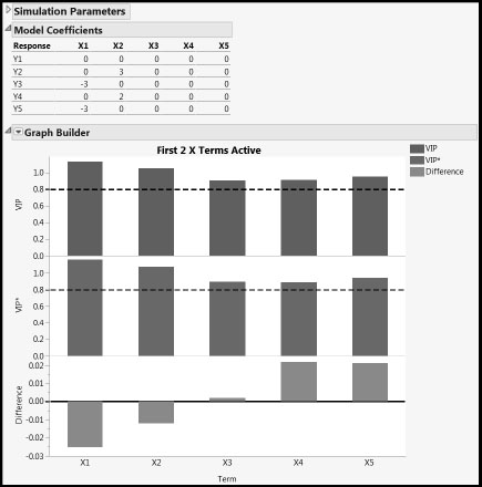
Run the script under several conditions to see the effect, and then close any open reports before continuing.

The Standardize X Option

This option is available only on the Fit Model launch window, when Partial Least Squares is selected as the personality. It is of interest if you construct model terms from the columns in your data table. Suppose that you have two columns, X₁ and X₂, and that you are interested in including interaction or polynomial terms. For an example, suppose that you add the term X₁ * X₂ as an effect in the Fit Model launch window.

The Center and Scale options construct the product using the raw measurements in the columns X₁ and X₂. If only these options are selected, the product is centered and scaled, so that the variable that enters the PLS calculation is

$\frac{X_1{X}_2-mean(X_1{X}_2)}{stdev(X_1{X}_2)}$

But, if you center and scale your columns, you might want to form polynomial terms from centered and scaled columns, rather than from the original data values. When you enter the term X₁ * X₂ in the Fit Model launch window, the Standardize X option inserts this term into the model:

$\left(\frac{X_1-mean(X_1)}{stdev(X_1)}\right)*\left(\frac{X_2-mean(X_2)}{stdev(X_2)}\right)$

This product is then centered and scaled based on selection of the Center and Scale options.

The three options Center, Scale, and Standardize X are checked by default in the Fit Model launch window. If all of your effects are main effects, the models fit with and without the Standardize X option are identical.

Determining the Number of Factors

Cross Validation: How JMP Does It

Cross validation is based on the Predicted Residual Sums of Squares (PRESS) statistic. This section illustrates the calculation of this statistic.

Suppose that you specify KFold as the Validation Method and set the Number of Folds to h. We will describe how the Root Mean PRESS values, found in the KFold Cross Validation report, are calculated. Note that, when you run the model with KFold as the Validation Method, under the report for the suggested fit, you are given the option to Save Columns > Save Validation. This saves a column containing an identifier for the holdout set to which a given row belongs.

Specify a number of factors, say a factors. The Root Mean PRESS value for a factors can be calculated as follows:

1. Exclude the observations in the ith holdout set.

1. Fit a model with a factors to the remaining observations, specifying None as the Validation Method.

2. Save the prediction formulas for this model by selecting Save Columns > Save Prediction Formula.

3. For each of the k Ys, calculate PRESS values for that response for the observations in the ith fold as follows: Compute the squared difference between the observed value and the predicted value (the squared prediction error), and divide the result by the variance for the entire response column.

4. Sum the means of these values across the h holdout sets and divide the sum of these means by the number of folds minus one. Call the result PRESS(Y).

5. The Root Mean PRESS is the square root of the mean of the PRESS(Y) values across the k responses.

The data table WaterQuality_PRESSCalc.jmp illustrates the calculation of the Root Mean PRESS for a NIPALS model with 2 factors. You can open this table by clicking on the correct link in the master journal. For simplicity, we have selected two of the responses from the WaterQuality.jmp data table in Chapter 7, HAB and RICH, and 47 rows from the original data table.

Run the PLS Fit script. This script contains a random seed, so that you can obtain the same results as are shown in the data table. The KFold Cross Validation with K=2 and Method = NIPALS report shows the Root Mean PRESS values that appear in Figure 2.

Figure A1.2: Cross Validation Report

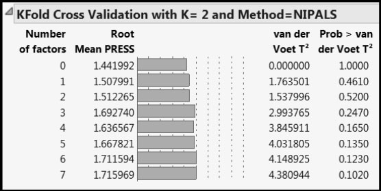
The data table WaterQuality_PRESSCalc.jmp contains steps for the calculation of the Root Mean PRESS value for Number of factors equal to 2, namely 1.512265. Note that the column called Validation in the data table is precisely the validation column associated with this specific report. To verify this, from the NIPALS Fit with 2 Factors red triangle menu, select Save Columns > Save Validation. Once you have verified that you obtain the same fold assignments, you can delete the column you have added (Validation 2).

Run the script Predictions Fold 1. This script excludes the observations in Validation fold 2, and fits a two-factor NIPALS model on only the data in Validation fold 1. It saves the prediction formulas in columns called Pred Formula HAB_2 and Pred Formula RICH_2, where the “2” indicates that these are applied to the test data in fold 2. Run Predictions Fold 2. This script saves prediction formulas built using the data in fold 2 in columns called Pred Formula HAB_1 and Pred Formula RICH_1.

Now run the script PRESS Calculations. This saves formulas to the data table that accomplish the calculations described in steps 4 through 6 above. The final column, RM PRESS 2 Factors, shows the value 1.512265, which is the value shown in Figure A1.2.

For details about the van der Voet test, see the SAS/STAT 9.3 User’s Guide and search for “van der Voet”.