Chapter 6: Introducing Structured Streaming
Many organizations have a need to consume large amounts of data continuously in their everyday processes. Therefore, in order to be able to extract insights and use the data, we need to be able to process this information as it arrives, resulting in a need for continuous data ingestion processes. These continuous applications create a need to overcome challenges such as creating a reliable process that ensures the correctness of the data, despite possible failures such as traffic spikes, data not arriving in time, upstream failures, and so on, which are common when working with continuously incoming data or transforming data without consistent file formats that have different structure levels or need to be aggregated before being used.
The most traditional way of dealing with these issues was to work with batches of data executed in periodic tasks, which processed raw streams and data and stored them into more efficient formats to allow queries on the data, a process that might incur high latency.
In this chapter, we will learn about Structured Streaming, which is the Apache Spark application programming interface (API) that allows us to make computations on streaming data in the same way you would express a batch computation on static data. Structured Streaming is a fault-tolerant engine that allows us to perform optimized operations for low-latency Structured Query Language (SQL)-like queries on the data thanks to the use of Spark SQL, while ensuring data consistency.
We can use Structured Streaming when creating ETL pipelines that will allow us to filter, transform, and clean data as it comes in a raw structure, formatting data types into more efficient storage formats, applying efficient partition strategies based on relevant columns, and so on. Specifically, in this chapter, we will look at the following topics:
- Using the Structured Streaming API
- Using different sources available in Azure Databricks when dealing with continuous streams of data
- Recovering from query failures
- Optimizing streaming queries
- Triggering streaming query executions
- Visualizing data on streaming dataframes
- Example on Structured Streaming
Without further ado, we will start our discussion by talking about Structured Streaming models and how can we leverage their architecture to improve performance when working with streams of data.
Technical requirements
This chapter will require you to have an Azure Databricks subscription available to work on the examples, as well as a notebook attached to a running cluster.
Let's start by looking into Structured Streaming models in more detail to find out which alternatives are available to work with streams of data in Azure Databricks.
Structured Streaming model
A Structured Streaming model is based on a simple but powerful premise: any query executed on the data will yield the same results as a batch job at a given time. This model ensures consistency and reliability by processing data as it arrives in the data lake, within the engine, and when working with external systems.
As seen before in the previous chapters, to use Structured Streaming we just need to use Spark dataframes and the API, stating which are the I/O locations.
Structured Streaming models work by treating all new data that arrives as a new row appended to an unbound table, thereby giving us the opportunity to run batch jobs on data as if all the input were being retained, without having to do so. We then can query the streaming data as a static table and output the result to a data sink.
Structured Streaming is able to do this, thanks to a feature called Incrementalization, which plans a streaming execution every time that we run a query. This also helps to figure out which states need to remain updated every time new data arrives.
We define when the tables will be updated using specific triggers when using Structured Streaming dataframes. Each time a trigger is activated, Azure Databricks will update the table incrementally by creating new rows for each file that arrives in our data source.
Finally, the last part to be defined are the output modes. These modes allow us to determine how to write incrementally to external systems such as Simple Storage Service (S3) or a database in three different ways, outlined as follows:
- Append mode: Only new rows are appended. This mode doesn't allow changes to existing rows.
- Complete mode: The entire table is rewritten to the external storage every time there is an update.
- Update mode: Only rows that have changed since the last trigger are written to the external storage, which allows in-place updates such as SQL tables.
Structured Streaming output tables provide consistent results based on a sequential stream, and failure tolerance is also ensured when working with output sinks. Using the Complete output mode, for example, out-of-order data will be handled by updating the records in a SQL table. We can establish a threshold to avoid overly old data updating a table.
Structured Streaming is a fault-tolerant system that allows queries to be run incrementally on streaming data, as explained in the following examples:
- For example, if we want to read JavaScript Object Notation (JSON) files that arrive continuously at an S3 location, we write the following code:
input_df = spark.readStream.json("s3://datalogs")
- We can operate on the Spark dataframe and do time-based aggregations to finally write to a SQL database, as follows:
input_df.groupBy($"message", window("update_time",
"1 hour")).count()
.writeStream.format("jdbc").start(jdbc_conn_string)
- If we run this as a batch operation, the only changes will be about how we write and read the data. For example, to read the data just once, run the following code:
input_df = spark.read.json("s3://datalogs")
- Then, we can do operations using the standard Spark DataFrame API and write to a SQL database, as illustrated in the following code snippet:
inputDF.groupBy("message", window("update_time",
"1 hour")).count()
.writeStream.format("jdbc").save(jdbc_conn_string)
In the next section, we will see in detail how to use the Structured Streaming API in more detail, including how to perform interactive queries and windowed aggregations, and we will discuss mapping and filtering operations.
Using the Structured Streaming API
Structured Streaming is integrated into the PySpark API and embedded in the Spark DataFrame API. It provides ease of use when working with streaming data and, in most cases, it requires very small changes to migrate from a computation on static data to a streaming computation. It provides features to perform windowed aggregation and for setting the parameters of the execution model.
As we have discussed in previous chapters, in Azure Databricks, streams of data are represented as Spark dataframes. We can verify that the data frame is a stream of data by checking that the isStreaming property of the data frame is set as true. In order to operate with Structured Streaming, we can summarize the steps as read, process, and write, as exemplified here:
- We can read streams of data that are being dumped in, for example, an S3 bucket. The following example code shows how we can use the readStream method, specifying that we are reading a comma-separated values (CSV) file stored in the S3 Uniform Resource Interface (URI) passed:
input_df=spark.readStream.csv("s3://data_stream_uri")
The resulting PySpark dataframe, input_df, will be the input table, continuously extended with new rows as new files arrive in the input directory. We will suppose that this table has two columns—update_time and message.
- Now, you can use the usual data frame operations to transform the data as if it were static. For example, if we want to count action types of each hour, we can do this by grouping the data by message and 1-hour windows of time, as illustrated in the following code snippet:
counts_df = input_df.groupBy($"message", window($"update_time ", "1 hour")).count()
The new dataframe, counts_df, is our result table, which has message, window, and counts columns, and will be continuously updated when the query is started. Note that this operation will yield the resulting hourly counts even if input_df is a static table. This is a feature that provides a safe environment to test a business logic on static datasets and seamlessly migrate into streaming data without changing the logic.
- Finally, we write this table to a sink and start the streaming computation by creating a connection to a SQL database using a Java Database Connectivity (JDBC) connection string, as illustrated in the following code snippet:
final_query = counts_df.writeStream.format("jdbc").start("jdbc://...")
The returned query is a StreamingQuery query, which is a handle to the active streaming execution running in the background. It can later be used to manage and monitor the execution of our streaming query. Beyond these basics, there are many more operations that can be done in Structured Streaming.
Mapping, filtering, and running aggregations
Structured Streaming allows the use of mapping, filtering, selection, and other methods to transform data. In the previous example, we used one of these features: time-based aggregations on data through the Spark API. As we have seen in our previous example, aggregations such as windowing can be expressed as a simple group by operations on a data frame. The use of such operations will be exemplified in the next section, but it is good to remember that Structured Streaming allows us to perform mapping, filtering, and other data-wrangling methods in the same way as with a common PySpark dataframe.
In the next section, we will see some examples of how these operations are performed using Structured Streaming.
Windowed aggregations on event time
When working with data that has a temporal dimension, compute operations often need to be windowed to certain periods of time, which in cases such as sliding windows overlap with each other. For example, we might need to perform operations over a window of 1 hour that slides forward every 5 minutes.
Windows are specified using the window function in a PySpark dataframe. For example, change to a sliding window approach (shown in the example previously given in the Structured Streaming model section) by doing the following:
input_df.groupBy("message", window("update_time", "1 hour",
"5 minutes")).count()
In the way our previous example was structured, the resulting information was formatted as (hour, message, count); now, it will have the form (window, message, count). Out-of-order data arriving late will be processed and the results will be updated accordingly, and if we are using an external data sink in Complete mode, the data will be updated there as well.
Merging streaming and static data
As we have mentioned before, working with Structured Streaming means working with Spark data frames, which is straightforward and allows us to use streaming and static data in combination. For example, if we have a table named users and we want to append it to a streaming data frame we can do the following, where we bring in a table called users and append it to our input_df dataframe:
users_df = spark.table("users")
input_df.join(users_df, "user_id").groupBy("user_name", hour("time")).count()
We could also create this static data frame using a query and run it in the same batch and streaming operations.
Interactive queries
In Structured Streaming, we can make use of the results from computations directly to interactive queries using the Spark JDBC server. There is an option to use a small memory sink designed for small amounts of data, whereby we can write results to a SQL table and then query the data in it. For example, we can create a table named message_counts that can be used as a small data sink that we can later query.
We do this by creating an in-memory table, as follows:
message_counts.writeStream.format("memory")
.queryName("user_counts")
.outputMode("complete")
.start()
And then, we use a SQL statement to query it, like this:
%sql
select sum(count) from message_counts where message='warning'"
In the next section, we will discuss all the different sources from where we can read stream data.
Using different sources with continous streams
Streams of data can come from a variety of sources. Structured Streaming provides support from extracting data from sources such as Delta tables, publish/subscribe (pub/sub) systems such as Azure Event Hubs, and more. We will review some of these sources in the next sections to learn how we can connect these streams of data into our jobs running in Azure Databricks.
Using a Delta table as a stream source
As mentioned in the previous chapter, you can use Structured Streaming with Delta Lake using the readStream and writeStream Spark methods, with a particular focus on overcoming issues related to handling and processing small files, managing batch jobs, and detecting new files efficiently.
When a Delta table is used as a data stream source, all the queries done on that table will process the information on that table as well as any data that has arrived since the stream started.
In the next example, we will load both the path and the tables into a dataframe, as follows:
df = spark.readStream.format("delta").load("/mnt/delta/data_events")
Or, we can do the same by referencing the Delta table, as follows:
df = spark.readStream.format("delta").table('data_events')
One of the features of Structured Streaming in Delta Lake is that we can control the maximum number of new files to be considered every time a trigger is activated. We can control this by setting the maxFilesPerTrigger option to the desired number of files to be considered. Another option to set is the rate limit on how much data gets to be processed in every micro-batch. This is controlled by using the maxBytesPerTrigger option, which controls the number of bytes processed each time the trigger is activated. The number of bytes to be processed will approximately match the number specified in this option, but it can slightly surpass this limit.
One thing to mention is that Structured Streaming will fail if we attempt to append a column or modify the schema of a Delta table that is being used as the source. If changes need to be introduced, we can approach this in two different ways, outlined as follows:
- After the changes are made, we can delete the output and checkpoint and restart the stream from the start.
- We can use the ignoreDeletes option to ignore operations that causes the deletion of data, or ignoreChanges so that the stream doesn't get interrupted by deletions or updates in the source table.
For example, suppose that we have a table named user_messages from where we stream out data that contains date, user_email, and message columns partitioned by date. If we need to delete data at partition boundaries, which means deleting using a WHERE clause on the partition column, the files are already segmented by that column. Therefore, the delete operation will just remove those files from the metadata.
So, if you just want to delete data using a WHERE clause on a partition column, you can use the ignoreDeletes option to avoid having your stream disrupted, as illustrated in the following code snippet:
data_events.readStream
.format("delta").option("ignoreDeletes", "true")
.load("/mnt/delta/user_messages")
However, if you have to delete data based on the user_email column, then you will need to use the following code:
data_events.readStream
.format("delta").option("ignoreChanges", "true")
.load("/mnt/delta/user_messages")
If you update a user_email variable with an UPDATE statement, the file that contains that record will be rewritten. If the ignoreChanges option is set to true, this file will be processed again, inserting the new record and other already processed records into the same file, producing duplicates downstream. Thus, it is recommended to implement some logic to handle these incoming duplicate records.
In order to specify a starting point of the Delta Lake streaming source without processing the entire table, we can use the following options:
- startingVersion: The Delta Lake version to start from
- startingTimestamp: The timestamp to start from
We can choose between these two options but not use both at the same time. Also, the changes made by setting this option will only take place once a new stream has been started. If the stream was already running and a checkpoint was written, these options would be ignored:
- For example, suppose you have a user_messages table. If you want to read changes since version 10, you can use the following code:
data_events.readStream
.format("delta").option("startingVersion", "10")
.load("/mnt/delta/user_messages")
- If you want to read changes since 2020-10-15, you can use the following code:
data_events.readStream
.format("delta")option("startingTimestamp", "2020-10-15")
.load("/mnt/delta/user_messages")
Keep in mind that if you set the starting point using one of these options, the schema of the table will still be the latest one of the Delta table, so we must avoid creating a change that makes the schema incompatible. Otherwise, the streaming source will either yield incorrect results or fail when reading the data.
Using Structured Streaming allows us to write into Delta tables and, thanks to the transaction log, Delta Lake will guarantee exactly once processing is done, even with several queries being run against the streaming table.
By default, Structured Streaming runs in Append mode, which adds new records to the table. This option is controlled by the outputMode parameter.
For example, we can set the mode to "append" and reference the table using the path method, as follows:
data_events.writeStream.format("delta")
.outputMode("append")
.option("checkpointLocation", "/delta/data_events/_checkpoints/etl-from-json")
.start("/delta/data_events")
Or, we could use the table method, as follows:
data_events.writeStream.format("delta")
.outputMode("append")
.option("checkpointLocation", "/delta/data_events/_checkpoints/etl-from-json")
.table("data_events")
We can use Complete mode in order to reprocess all the information available on a table. For example, if we want to aggregate the count of users by user_id value every time we update the table, we can set the mode to complete and the entire table will be reprocessed in every batch, as illustrated in the following code snippet:
spark.readStream.format("delta")
.load("/mnt/delta/data_events")
.groupBy("user_id").count()
.writeStream.format("delta")
.outputMode("complete")
.option("checkpointLocation", "/mnt/delta/messages_by_user/_checkpoints/streaming-agg")
.start("/mnt/delta/messages_by_user")
This behavior can be better controlled using one-time triggers that allow us to have fine-grained control on what the actions are that should trigger the table update. We can use them in applications such as aggregation tables or with data that needs to be processed on a daily basis.
Azure Event Hubs
Azure Event Hubs is a telemetry service that collects, transforms, and stores events. We can use it to ingest data from different telemetry sources and to trigger processes in the cloud.
There are many ways to establish a connection. One way is to use ConnectionStringBuilder to make your connection string. To do this, follow these steps:
- The following Scala code shows how we can establish a connection using ConnectionStringBuilder by defining parameters such as the event hub name, shared access signature (SAS) key, and key name:
import org.apache.spark.eventhubs.ConnectionStringBuilder
val connections_string = ConnectionStringBuilder()
.setNamespaceName("your_namespace-name")
.setEventHubName("event_hub-name")
.setSasKeyName("your_key-name")
.setSasKey("your_key build
In order to create this connection, we need to install the Azure Event Hubs library in the Azure Databricks workspace in which you are using Maven coordinates. This connector is updated regularly, so to check the current version, go to Latest Releases in the Azure Event Hubs Spark Connector project README file.
- After we have set up our connection, we can use it to start streaming data into the Spark dataframe. The following Scala code shows how we first define the Event Hubs configuration:
val event_hub_conf = EventHubsConf(connections_string)
.setStartingPosition(EventPosition.fromEndOfStream)
- Finally, we can start streaming into our dataframe, as follows:
var streaming_df =
spark.readStream
.format("eventhubs").options(event_hub_conf.toMap)
.load()
- You can also define this using Python and specifying the connection string to Azure Event Hubs and then start to read the stream of that directly, as follows:
conf = {}
conf["eventhubs.connectionString"] = ""
stream_df = spark
.readStream
.format("eventhubs")
.options(**conf)
.load()
Here, we have created a connection and used this to read the stream directly from the Azure event hub specified in the connection string.
Establishing a connection between Azure Event Hubs allows you to aggregate the telemetry of different sources being tracked into a single Spark data frame that can be later on be processed and consumed by an application or stored for analytics.
Auto Loader
Auto Loader is an Azure Databricks feature used to incrementally process data as it arrives at Azure Blob storage, Azure Data Lake Storage Gen1, or Azure Data Lake Storage Gen2. It provides a Structured Streaming source named cloudFiles that, when given an input directory path on the cloud file storage, automatically processes files as they arrive in it, with the added option of also processing existing files in that directory.
Auto Loader uses two modes for detecting files as they arrive at the storage point, outlined as follows:
- Directory listing: This lists all files into the input directory. It might become too slow when the number of files in the storage grows too large.
- File notification: This creates an Azure Event Hubs notification service to detect new files when they arrive in the input directory. This is a more scalable solution for large input directories.
The file detection mode can be changed when the stream is restarted. For example, if the Directory listing mode starts to slow down, we can change it to File notification. On both modes, Auto Loader will keep track of the files to guarantee that these are processed only once.
The cloudFiles option can be set in the same way as for other streaming sources, as follows:
df = spark.readStream.format("cloudFiles")
.option(<cloudFiles-option>, <option-value>)
.schema(<schema>).load(<input-path>)
After changing the file detection mode, we can start a new stream by writing it back again to a different checkpoint path, like this:
df.writeStream.format("delta")
.option("checkpointLocation", <checkpoint-path>).start(<output-path>)
Next, we will see how we can use Apache Kafka in Structured Streaming as one of its sources of data.
Apache Kafka
Pub/sub messaging systems are used to provide asynchronous service-to-service communication. They are used in serverless and microservices architectures to construct event-driven architectures. In these systems, messages published are immediately received by all subscribers to the topic.
Apache Kafka is a distributed pub/sub messaging system that consumes live data streams and makes them available to downstream stakeholders in a parallel and fault-tolerant fashion. It's very useful when constructing reliable live-streaming data pipelines that need to work with data across different processing systems.
Data in Apache Kafka is organized into topics that are in turn split into partitions. Each partition is an ordered sequence of records that resembles a commit log. As new data arrives at each partition in Apache Kafka, each record is assigned a sequential ID number called an offset. The data in these topics is retained for a certain amount of time (called a retention period), and it's a configurable parameter.
The seemingly infinite nature of the system means that we need to decide the point in time from where we want to start read our data. For this, we have the following three choices:
- Earliest: We will start reading our data at the beginning of the stream, excluding data that is older than the retention period deleted from Kafka.
- Latest: We will process only new data that arrives after the query has started.
- Per-partition assignment: With this, we specify the precise offset to start from for every partition, to control the exact point in time from where the processing should start. This is useful when we want to pick up exactly where a process failed.
The startingOffsets option accepts just one of these options and is only used on queries that start from a new checkpoint. A query that is restarted from an existing checkpoint will always resume where it was left off, except when the data at that offset is older than the retention period.
One advantage when using Apache Kafka in Structured Streaming is that we can manage what to do when the stream first starts and what to do if the query is not able to pick up from where it left off because the data is older than the retention period, using the startingOffsets and failOnDataLoss options, respectively. This is set with the auto.offset.reset configuration option.
In Structured Streaming, you can express complex transformations such as one-time aggregation and output the results to a variety of systems. As we have seen, using Structured Streaming with Apache Kafka allows you to transform augmented streams of data read from Apache Kafka using the same APIs as when working with batch data and integrate data read from Kafka, along with data stored in other systems including such as S3 or Azure Blob storage.
In order to work with Apache Kafka, it is recommended that you store your certificates in Azure Blob storage or Azure Data Lake Storage Gen2, to be later accessed using a mount point. Once your paths are mounted and you have already stored your secrets, you can connect to Apache Kafka by running the following code:
streaming_kafka_df = spark.readStream.format("kafka")
.option("kafka.bootstrap.servers", ...)
.option("kafka.ssl.truststore.location",<dbfs-truststore-location>)
.option("kafka.ssl.keystore.location", <dbfs-keystore-location>)
.option("kafka.ssl.keystore.password", dbutils.secrets.get(scope=<certificate-scope-name>,key=<keystore-password-key-name>))
.option("kafka.ssl.truststore.password", dbutils.secrets.get(scope=<certificate-scope-name>,key=<truststore-password-key-name>))
To write into Apache Kafka, we can use writeStream on any PySpark dataframe that contains a column named value and, optionally, a column named key. If a key column is not specified, then a null-valued key column will be automatically added. Bear in mind that a null-valued key column may lead to uneven partitions of data in Kafka, so you should be aware of this behavior.
We can specify the destination topic either as an option to DataStreamWriter or on a per-record basis as a column named topic in the dataframe.
In the following code example, we write key-value data from a dataframe into a specified Kafka topic:
query = streaming_kafka_df
.selectExpr("CAST(user_id AS STRING) AS key", "to_json(struct(*)) AS value")
.writeStream
.format("kafka")
.option("kafka.bootstrap.servers", "host1:port1,host2:port2")
.option("topic", "topic1")
.option("checkpointLocation", path_to_HDFS).start()
The preceding query takes a dataframe containing user information and writes it to Kafka. user_id is a string used as the key. In this operation, we are transforming all the columns of the dataframe into JSON strings, putting the results in the value of the record.
In the next section, we will learn how to use Avro data in Structured Streaming.
Avro data
Apache Avro is a commonly used data serialization system. We can use Avro data in Azure Databricks using the from_avro and to_avro functions to build streaming pipelines that encode a column into and from binary Avro data. Similar to from_json and to_json, you can use these functions with any binary column, but you must specify the Avro schema manually. The from_avro and to_avro functions can be passed to SQL functions in streaming queries.
The following code snippet shows how we can use the from_avro and to_avro functions along with streaming data:
from pyspark.sql.avro.functions import from_avro, to_avro
streaming_df = spark
.readStream
.format("kafka")
.option("kafka.bootstrap.servers", servers)
.option("subscribe", "t")
.load()
.select(
from_avro("key", SchemaBuilder.builder().stringType()).as("key"),
from_avro("value", SchemaBuilder.builder().intType()).as("value"))
In this case, when reading the key and value of a Kafka topic, we must decode the binary Avro data into structured data, which has the following schema: <key: string, value: int>.
We can also convert structured data to binary from string and int, which will be interpreted as the key and value, and later on save it to a Kafka topic. The code to do this is illustrated in the following snippet:
streaming_df.select(
to_avro("key").as("key"),
to_avro("value").as("value"))
.writeStream
.format("kafka")
.option("kafka.bootstrap.servers", servers)
.option("article", "t")
.save()
You can also specify a schema by using a JSON string to define the fields and its data types (for example, if "/tmp/userdata.avsc" is), as follows:
{
"namespace": "example.avro",
"type": "record",
"name": "User",
"fields": [
{"name": "name", "type": "string"},
{"name": " filter_value", "type": ["string", "null"]}
]
}
We can create a JSON string and use it in the from_avro function, as shown next. First, we specify the JSON schema to be read, as follows:
from pyspark.sql.avro.functions import from_avro, to_avro
json_format_schema = open("/tmp/ userdata.avsc", "r").read()
Then, we can use the schema in the from_avro function. In the following code example, we first decode the Avro data into a struct, filter by the filter_value column, and finally encode the name column in Avro format:
output = straming_df.
.select(from_avro("value", json_format_schema).alias("user"))
.where('user.filter_value == "value1"')
.select(to_avro("user.name").alias("value"))
The Apache Avro format is widely used in the Hadoop environment and it's a common option in data pipelines. Azure Databricks provides support for the ingestion and handling of sources using this file format.
The next section will dive into how we can integrate different data sinks in order to dump the data there, before and after it has been processed.
Data sinks
Sometimes, it is necessary to aggregate the receiving streams of data to be written into another location, which can be a data sink. Data sinks are a way in which we can call external sources where we store data and can be, for example, an S3 bucket where we want to keep copies of the aggregated streams of data. In this section, we will go through the steps in which we can write the streams of data into any external data sink location.
In Structured Streaming APIs, we have two ways to write the output of a query to external data sources that do not have an existing streaming sink. These options are the foreachBatch and foreach functions.
The foreachBatch method of writeStream allows existing batch data sources to be reused. This is done by specifying a function that is executed on the output data of every micro-batch of the streaming query. This function takes two parameters: the first parameter is the data frame that has the output data of a micro-batch, and the second one is the unique ID of that micro-batch. The foreachBatch method allows you to do the following:
- Reuse existing batch data sources.
- Write to multiple locations.
- Apply additional data frame operations.
In a case where there might not be a streaming sink available in the storage system but we can write data in batches, we can use foreachBatch to write the data in batches.
We can also write the output of a streaming query to multiple locations. We can do so by simply writing the output data frame into these multiple locations, although this might lead to data being computed every time we write into a different location and possibly having to read all the input data again. To avoid this, we can cache the output data frame, then write to the location, and finally uncache it.
In the following code example, we see how we can write to different locations using foreachBatch in Scala:
streaming_df.writeStream.foreachBatch { (batchDF: DataFrame, batchId: Long) =>
batchDF.persist()
batchDF.write.format(format_location_1).save(your_location_1)
batchDF.write.format(format_location_2).save(your_location_2)
batchDF.unpersist()
}
The foreachBatch method helps us to overcome certain limitations regarding operations that are available for static DataFrames but not supported in streaming DataFrames. The foreachBatch option allows us to apply these operations to each micro-batch output.
The foreachBatch method guarantees data to be processed only once, although you can use the batchId parameter provided as a means to apply deduplication methods. It is important to also notice that one of the main differences between foreachBatch and foreach is that the former will not work for continuous processing modes as it fundamentally relies on micro-batch execution, while the latter gives an option to write data in continuous mode.
If, for some reason, foreachBatch is not an available option to use, then you can code your custom writer using the foreach option and have the data-writing logic be divided into open, process, and close methods.
In Python, we can make use of the foreach method either in a function or in an object. The function provides an effective way to code your processing logic but will not allow deduplicating of output data in the case of failure, causing the reprocessing of some input data. In that case, you should specify the processing logic within an object.
The following custom function takes a row as input and writes the row to storage:
def process_row (row):
"""
Custom function to write row to storage.
"""
pass
Then, we can use this function in the foreach method of writeStream, as follows:
query = streaming_df.writeStream.foreach(process_row).start()
To construct the object, it needs to have a process method that will write the row to the storage. We can also add optional open and close methods to handle the connection, as illustrated in the following code snippet:
class ForeachWriter:
def open(self, partition_id, epoch_id):
"""
Optional method to open the connection
"""
def process(self, row):
"""
Custom function to write row to storage. Required method.
"""
def close(self, error):
"""
Optional method to close the connection
"""
Finally, we can call this object on the query using the foreach method of writeStream, as illustrated in the following code snippet:
query = streaming_df.writeStream.foreach(ForeachWriter()).start()
In this way, we can very easily define a class with methods that process the streams of data we receive using Structured Streaming and then write to external locations that will be used as data sinks of the processed streams of data, using the writeStream method.
In the next section, we will go through the steps that we should follow in order to maintain integrity of the data, regardless of query failures or interruptions of the stream, by specifying the use of checkpoints.
Recovering from query failures
Failures can happen because of changes in the input data schema, changes along tables used in the computation, missing files, or due to many other root causes. When developing applications that make use of streams of data, it is necessary to have robust failure-handling methods. Structured Streaming guarantees that the results will remain valid even in the case of failure. To do this, it places two requirements on the input sources and output sinks, outlined as follows:
- The input sources should be replayable, which means that recent data can be read again if the job fails.
- The output sinks should allow transactional updates, meaning that these updates are atomic (while the update is running, the system should keep functioning) and can be rolled back.
One of the previously mentioned features of Structured Streaming is checkpointing, which can be enabled for streaming queries. This also allows a stream to quickly recover from a failure by simply restarting the stream after a failure, which will cause the query to continue from where it was left off, while guaranteeing data consistency. So, it is always recommended to configure Enable Query Checkpointing and to configure Databricks Jobs to restart your queries automatically after a failure.
To enable checkpointing, we can set the checkpointLocation option to the desired checkpoint path when writing the dataframe. An example of this is shown in the following code snippet:
streaming_df.writeStream
.format("parquet")
.option("path", output_path)
.option("checkpointLocation", checkpoint_path)
.start()
This checkpoint location preserves all information about a query. Therefore, all queries must have a unique checkpoint path.
We face limitations on the possible changes in a streaming query that are allowed between restarts using the same checkpoint path.
By saying that an operation is allowed, it is understood that we can implement the change, but whether the semantics or its effects will be as desired will depend on the query and the specific change applied.
The term not allowed means the change will likely fail when the query is restarted.
Here is a summary of the types of changes we can make:
- We are not allowed to change the number or type of input sources.
- If we can change parameters of input sources, this will depend on the source and query.
- Some changes in the type of output sink are allowed.
- If we can make changes to the parameters of the output sink, this will depend on the type of sink and query.
- Some changes are allowed on operations, such as map and filter operations.
- Changes in stateful operations can lead to failure due to changes in the schema of state data needed to update the result.
As we can see, Structured Streaming provides several features in order to provide fault tolerance for production-grade processing of streams of data.
In the next section, we will gain knowledge on how we can optimize the performance of our streaming queries.
Optimizing streaming queries
We can have a streaming query that makes use of stateful operations such as streaming aggregation, streaming dropDuplicates, mapGroupsWithState, or flatMapGroupsWithState, streaming to stream joins, and so on. Running these operations continuously results in a need to maintain millions of keys of the state of the data in the memory of each executor, leading to bottlenecks.
To overcome this issue, Azure Databricks provides a solution, which is to keep the state of the data in a RocksDB database instead of using the executor memory. RocksDB is a library that provides a persistent key-value store to efficiently manage the state of data in the memory and the local SSD. Therefore, used in combination with Structured Streaming checkpoints, these solutions guarantee safeguards against failures.
You can enable RocksDB-based state management by setting the following configuration in SparkSession before starting the streaming query:
spark.conf.set(
"spark.sql.streaming.stateStore.providerClass",
"com.databricks.sql.streaming.state.RocksDBStateStoreProvider")
RocksDB can maintain 100 times more state keys than the standard executor memory. We can also improve the performance of our queries using compute-optimized instances such as Azure Standard_F16s instances as workers and setting the number of shuffle partitions to up to two times the number of cores in the cluster.
Triggering streaming query executions
Triggers are a way in which we define events that will lead to an operation being executed on a portion of data, so they handle the timing of streaming data processing. These triggers are defined by intervals of time in which the system checks if new data has arrived. If this interval of time is too small this will lead to unnecessary use of resources, so it should always be an amount of time customized according to your specific process.
The parameters of the triggers of the streaming queries will define if this query is to be executed as a micro-batch query on a fixed batch interval or as a continuous processing query.
Different kinds of triggers
There are different kinds of triggers available in Azure Databricks that we can use to define when our streaming queries will be executed. The available options are outlined here:
- Unspecified trigger: This is the default option and means that unless specified otherwise, the query will be executed in micro-batch mode, where micro-batches are generated when the processing previous micro-batch has already been executed successfully.
- Triggers based on fixed-interval micro-batches: The query will be executed with micro-batches mode, where micro-batch execution will be started at specified intervals. If the previous micro-batch execution is completed in less than the specified interval, Azure Databricks will wait until the interval is over before kicking off the next micro-batch. If the execution of the micro-batch takes longer than the specified interval to complete, then the next batch will be executed as soon as the previous one is done.
If no new data is available, no micro-batch will be executed.
- One-time micro-batch triggers: The query will run just once to process all the available data. This is a good option when clusters are started and turned off to save resources, and therefore we can just process all the new data available since the start of the cluster.
- Continuous trigger with fix checkpoint interval: The query will be kicked off in a continuous low-latency processing mode.
Next, we will see some examples of how we can apply these different types of triggers when using Structured Streaming for streaming data.
Trigger examples
The following code snippet provides an example of the default trigger in Structured Streaming, which—as mentioned before—runs the micro-batch as soon as it can:
streaming_df.writeStream
.format("console")
.start()
We can also define a specific interval of time, making use of the processingTime trigger option. In the following code example, we set a 10-second micro-batch interval of time:
streaming_df.writeStream
.format("console")
.trigger(processingTime='10 seconds').start()
As mentioned before, we can set a one-time trigger to process all of our new data just once, as illustrated in the following code snippet:
streaming_df.writeStream
.format("console")
.trigger(once=True).start()
Finally, we can set a continuous trigger that will have a 2-second checkpointing interval of time for saving data, to recover from eventual failures. The code for this is illustrated in the following snippet:
streaming_df.writeStream
.format("console")
.trigger(continuous='1 second').start()
Triggers in Structured Streaming allow us to have fine-grained control over how our query will behave when processing new data that arrives in defined intervals of time.
In the last section of this chapter, we will dive into which tools are available in Azure Databricks to visualize data.
Visualizing data on streaming data frames
When working with streams of data in Structured Streaming data frames, we can visualize real-time data using the display function. This function is different from other visualizing functions because it allows us to specify options such as processingTime and checkpointLocation due to the real-time nature of the data. These options are set in order to manage the exact point in time we are visualizing and should be always be set in production in order to know exactly the state of the data that we are seeing.
In the following code example, we first define a Structured Streaming dataframe, and then we use the display function to show the state of the data every 5 seconds of processing time, on a specific checkpoint location:
streaming_df = spark.readStream.format("rate").load()
display(streaming_df.groupBy().count(), processingTime = "5 seconds", checkpointLocation = "<checkpoint-path>")
Specifically, these are the available parameters for this function:
- The streamName parameter is the specific streaming query in question that we want to visualize.
- The processingTime parameter defines the interval of time for how often the streaming query is executed. If it's not specified, Azure Databricks will check for the availability of new data when the previous process has been completed—a behavior that could lead to undesired cost increases. Therefore, this is an option that is recommended to be set explicitly when possible.
The checkpointLocation parameter is the path to where the checkpoint data is written. If not specified, the location will be temporary. It is recommended to set this parameter so that a stream can be restarted from where it was left in the case of any failure.
The Azure Databricks display function supports a variety of plot types. We can choose different types of plots by selecting the desired type of plot from the drop-down menu in the top-left corner of the cell where we executed the function, as illustrated in the following screenshot:

Figure 6.1 – Available options for the display function
We have an option to create different types of plots such as bar, scatter, and line plots, with the extra feature of being able to set options for these visualizations. If we click on the Plot Options menu, we will be prompted with a window where we can customize the plot depending on the selected type, as illustrated in the following screenshot:

Figure 6.2 – Available options for customizing a plot
The display option provides ease of use when visualizing data in general and streaming queries in particular. The provided options allow us to easily drag and drop the variables required to create each type of plot, selecting the type of aggregation executed and modifying several aspects of its design.
The next section will comprise of an example in which we will simulate a stream of data and use Structured Streaming to run streaming queries.
Example on Structured Streaming
In this example, we will be looking at how we can leverage knowledge we have acquired on Structured Streaming throughout the previous sections. We will simulate an incoming stream of data by using one of the example datasets in which we have small JSON files that, in real scenarios, could be the incoming stream of data that we want to process. We will use these files in order to compute metrics such as counts and windowed counts on a stream of timestamped actions. Let's take a look at the contents of the structured-streaming example dataset, as follows:
%fs ls /databricks-datasets/structured-streaming/events/
You will find that there are about 50 JSON files in the directory. You can see some of these in the following screenshot:
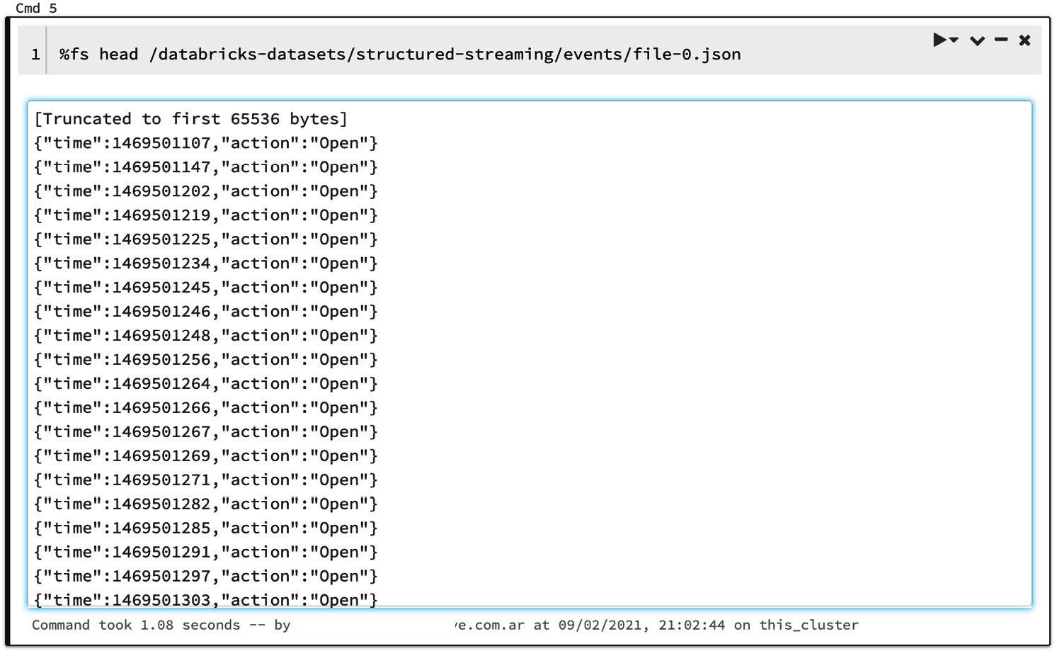
Figure 6.3 – The structured-streaming dataset's JSON files
We can see what one of these JSON files contains by using the fs head option, as follows:
%fs head /databricks-datasets/structured-streaming/events/file-0.json
We can see that each line in the file has two fields, which are time and action, so our next step will be to try to analyze these files interactively using Structured Streaming, as follows:
- The first step that we will take is to define the schema of our data and store it in a JSON file that we can later use to create a streaming dataframe. The code for this can be seen in the following snippet:
from pyspark.sql.types import *
input_path = "/databricks-datasets/structured-streaming/events/"
- Since we already know the structure of the data we won't need to infer the schema, so we will use PySpark SQL types to define the schema of our future streaming dataframe, as illustrated in the following code snippet:
json_schema = StructType([StructField("time",
TimestampType(),
True),
StructField("action",
StringType(),
True)])
- Now, we can build a static data frame using the schema defined before and loading the data in the JSON files, as follows:
static_df = (
spark
.read
.schema(json_schema)
.json(input_path)
)
- Finally, we can visualize the data frame using the display function, as mentioned in the previous section, as follows:
display(static_df)
The output is as follows:
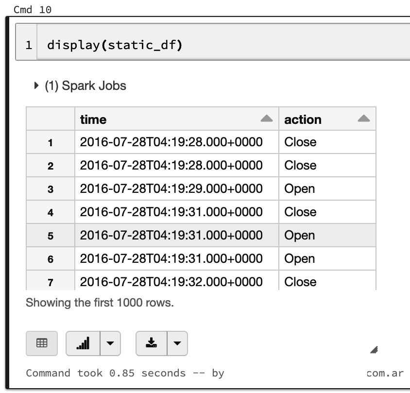
Figure 6.4 – Streaming data frame
- We are now ready to run the computation in order to know the amount of open and close orders by grouping data based on windowed aggregations of 1 hour. We will import everything from PySpark SQL functions using an asterisk (*) to get, among others, the window function, as illustrated in the following code snippet:
from pyspark.sql.functions import *
static_count_df = (
static_df
.groupBy(
static_df.action,
window(static_df.time, "1 hour"))
.count()
)
static_count_df.cache()
- Next, we register the dataframe as a temporary view called data_counts, as illustrated in the following code snippet:
static_count_df.createOrReplaceTempView("data_counts")
- Finally, we can directly query the table using SQL commands. For example, to compute the total counts throughout all the hours, we can run the following SQL command:
%sql
select action, sum(count) as total_count from data_counts group by action
The output is as follows:
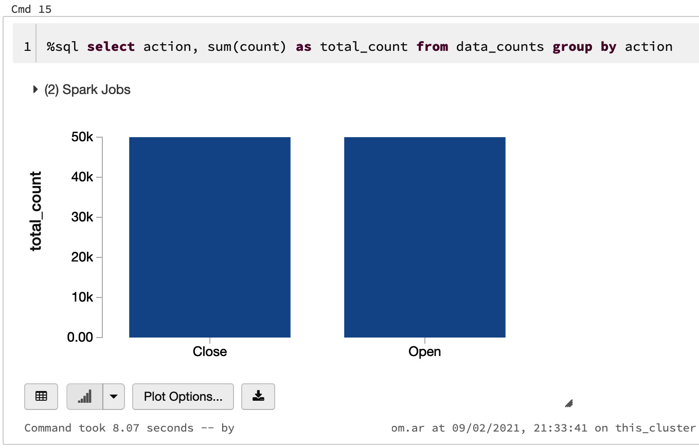
Figure 6.5 – SQL queries on a streaming data frame
- We can also use windowed counts to create a timeline grouped by time and action, as follows:
%sql
select action, date_format(window.end, "MMM-dd HH:mm") as time, count from data_counts order by time, action
The output is as follows:
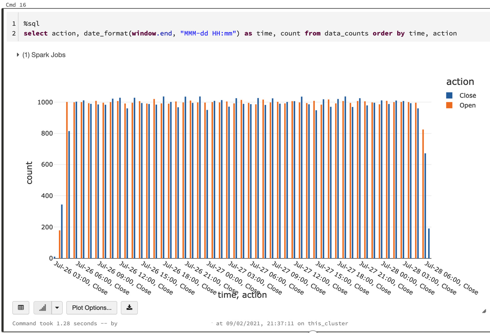
Figure 6.6 – Windowed counts on a streaming data frame
- In the following code example, we will use a similar definition to the one used here but using the readStream option instead of the read method. Also, in order to simulate a stream of files, we will pick one file at a time using the maxFilesPerTrigger option and setting it to 1:
from pyspark.sql.functions import *
streaming_df = (
spark
.readStream
.schema(json_schema)
.option("maxFilesPerTrigger", 1)
.json(input_path)
)
- We can then make the same query that we have applied to the static dataframe previously, as follows:
streaming_counts_df = (
streaming_df
.groupBy(
streaming_df.action,
window(streaming_df.time, "1 hour"))
.count()
)
- We can check that the data frame is actually a streaming source of data by running the following code:
streaming_df.isStreaming
The output is as follows:
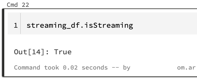
Figure 6.7 – Checking if the dataframe is a streaming source
As you can see, the output of streamingCountsDF.isStreaming is True, therefore streaming_df is a streaming dataframe.
- The next option is set, to keep the size of shuffles small, as illustrated in the following code snippet:
spark.conf.set("spark.sql.shuffle.partitions", "2")
- We can then store the results of our query, passing as format "memory" to store the result in an in-memory table. The queryName option will set the name of this table to data_counts. Finally, we set the output mode to complete so that all counts are on the table. The code can be seen in the following snippet:
query =
streaming_counts_df
.writeStream
.format("memory")
.queryName("data_counts")
.outputMode("complete")
.start()
The query object is a handle that runs in the background, continuously looking for new files and updating the windowed resulting aggregation counts.
Note the status of query in the preceding code snippet. The progress bar in the cell shows the status of the query, which in our case is active.
- We will artificially wait some time for a few files to be processed and then run a query to the in-memory data_counts table. First, we introduce a sleep of 5 seconds by running the following code:
from time import sleep
sleep(5)
- Then, we can run a query in another cell as a SQL command, using SQL magic, as follows:
%sql
select action, date_format(window.end, "MMM-dd HH:mm") as time, count
from data_counts
order by time, action
The following screenshot shows us the resulting graph created by running this query in one of the Databricks notebook code cells:
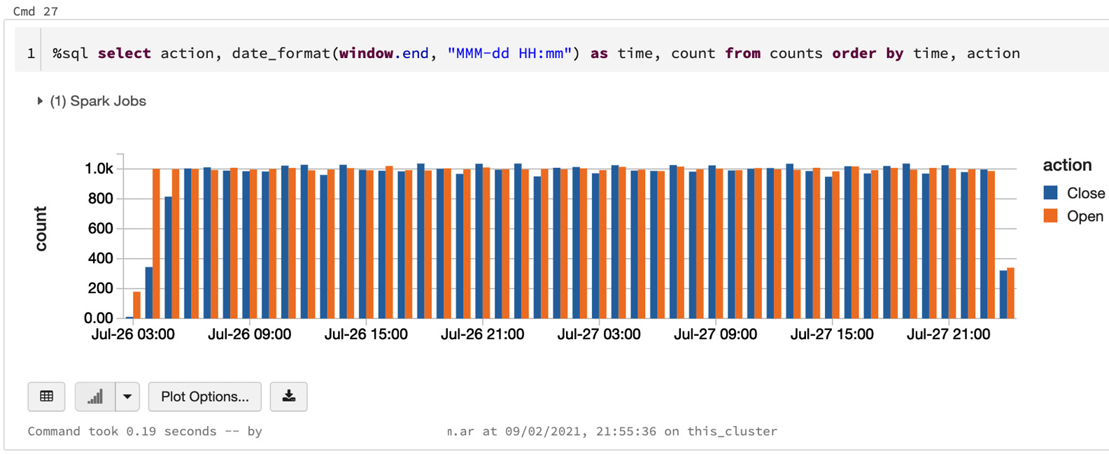
Figure 6.8 – The counts before waiting
We can see the timeline of windowed counts growing bigger. Running these queries will always result in the latest updated counts, which the streaming query is updating in the background.
- If we wait a few seconds more, we will have new data computed into the result table, as illustrated in the following code snippet:
sleep(5)
- And then, we run the query again, as follows:
%sql
select action, date_format(window.end, "MMM-dd HH:mm") as time, count
from data_counts
order by time, action
We can see in the following screenshot of a graph created by running the query that the results at the right side of the graph have changed as more data is being ingested:
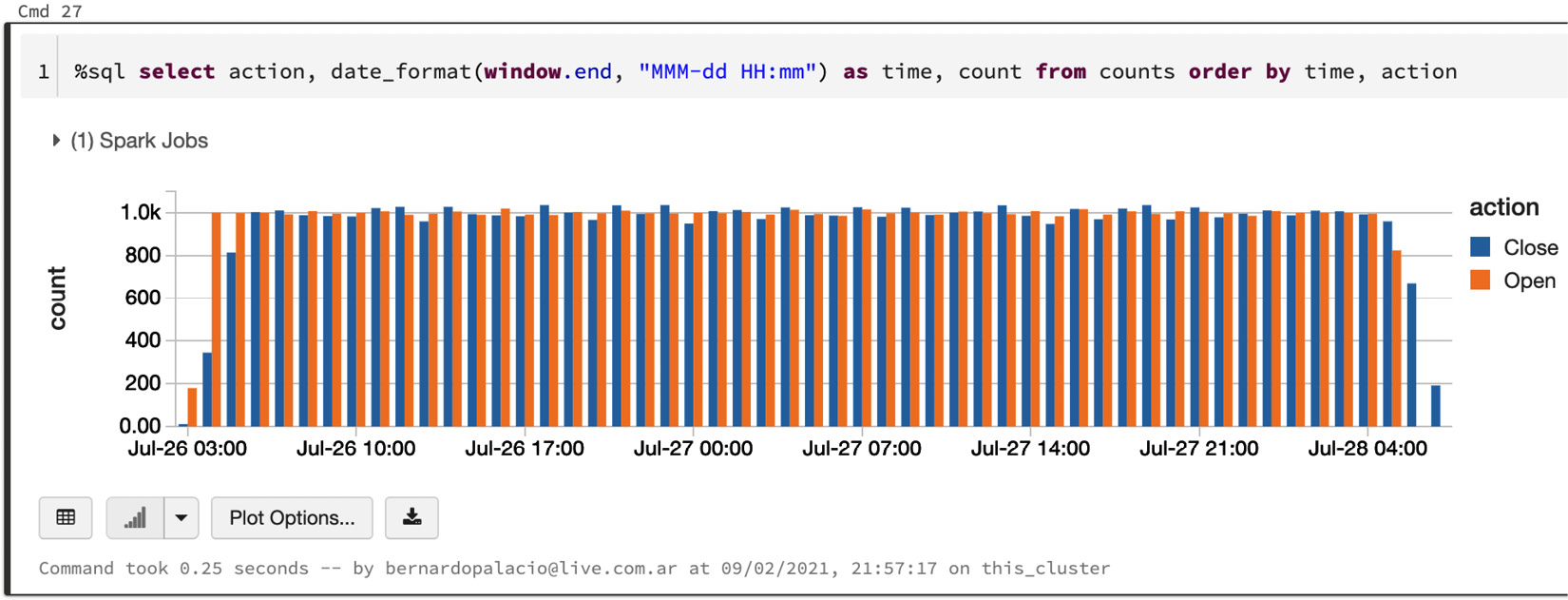
Figure 6.9 – The counts after waiting
- We can also see the resulting number of "opens" and "closes" by running the following SQL query:
%sql
select action, sum(count) as total_count
from data_counts
group by action order by action
This example has its limitations due to the small number of files present in the dataset. After consuming them all, there will be no more updates to the table.
- Finally, we can stop the query running in the background, either by clicking on the Cancel link in the cell of the query or by executing the query.stop function, as illustrated in the following code snippet:
query.stop()
Either way, the status of the cell where the query is running will be updated to TERMINATED.
Summary
Throughout this chapter, we have reviewed different features of Structured Streaming and looked at how we can leverage them in Azure Databricks when dealing with streams of data from different sources.
These sources can be data from Azure Event Hubs or data derived using Delta tables as streaming sources, using Auto Loader to manage file detection, reading from Apache Kafka, using Avro format files, and through dealing with data sinks. We have also described how Structured Streaming provides fault tolerance while working with streams of data and looked at how we can visualize these streams using the display function. Finally, we have concluded with an example in which we have simulated JSON files arriving in the storage.
In the next chapter, we will dive more deeply into how we can use the PySpark API to manipulate data, how we can use Python popular libraries in Azure Databricks and the nuances of installing them on a distributed system, how we can easily migrate from Pandas into big data with the Koalas API, and—finally—how to visualize data using popular Python libraries.