Chapter 8: Databricks Runtime for Machine Learning
This chapter will be a deep dive into the development of classic machine learning algorithms to train and deploy models based on tabular data, exploring libraries and algorithms as well. The examples will be focused on the particularities and advantages of using Azure Databricks Runtime for Machine Learning (Databricks Runtime ML).
In this chapter we will explore the following concepts, which are focused on how we can extract and improve the features available in our data to train our machine learning and deep learning models. The topics that we will cover are listed here:
- Loading data
- Feature engineering
- Time-series data sources
- Handling missing values
- Extracting features from text
- Training machine learning models on tabular data
In the following sections, we will discuss the necessary libraries needed to perform the operations introduced, as well as providing some context on how best practices and some core concepts are related to them.
Without further ado, let's start working with machine and deep learning models in Azure Databricks.
Loading data
Comma-separated values (CSV) are the most widely used format for tabular data in machine learning applications. As the name suggests, it stores data arranged in the form of rows, separated by commas or tabs.
This section covers information about loading data specifically for machine learning and deep learning applications. Although we can consider these concepts covered in the previous chapters and sections, we will reinforce concepts around how we can read tabular data directly into Azure Databricks and which are the best practices to do this.
Reading data from DBFS
When training machine learning algorithms in a distributed computing environment such as Azure Databricks, the need to have shared storage becomes important, especially when working with distributed deep learning applications. Azure Databricks File System (DBFS) allows efficient access to data for any cluster using Spark and local file application programming interfaces (APIs):
In Azure Databricks, we have an option to choose a Machine Learning Runtime that provides a high-performance Filesystem in Userspace (FUSE) mount, which is a virtual filesystem that can be accessed in the /dbfs location by all cluster nodes. This allows for the process that is running in cluster nodes to read to the same location using the distributed storage system with local file APIs.
- For example, when we write a file to the DBFS location, as illustrated in the following code snippet, we are using the shared filesystem across all cluster nodes:
with open("/dbfs/tmp/test_dbfs.txt", 'w') as f:
f.write("This is ")
f.write("in the shared ")
f.write("file system. ")
- In the same way, we can read a file on the distributed filesystem using local file APIs, as illustrated in the following code snippet:
with open("/dbfs/tmp/test_dbfs.txt", "r") as f_read:
for line in f_read:
print(line)
- This way, we can display the output to the console, as shown in the following screenshot:

Figure 8.1 – Output of reading a file in the shared filesystem
When using Azure Databricks Runtime ML, we have the option to use the dbfs:/ml folder, which is a special folder that has been optimized to offer high-performance input/output (I/O) for deep learning operations. This is especially handy as a workaround to the limitation of supporting files that are smaller than 2 gigabytes (GB) in Azure Databricks, so it is recommended to save data in this folder.
We can load data for training and inference of machine and deep learning applications by reading from tables or local CSV files, as we will see in the next section. Once the data has been loaded, we have plenty of options to then convert it to Spark DataFrames, pandas DataFrames, or NumPy arrays.
In the next section, we will again go through how we can read CSV files to work with distributed deep learning applications in Azure Databricks.
Reading CSV files
One of the most frequent formats for machine learning data is CSV, and it's regularly used to hold tabular data. Here, we use the term tabular data to describe data structured as rows representing observations, which in turn are described using variables or attributes in the form of columns.
As we have seen in previous chapters, we have a number of ways to load a CSV file into Azure Databricks. The first option would be to import the data into a Spark DataFrame using the PySpark API to parse the data. The following piece of code will read the file stored in the specified databricks dataset folder in DBFS into a Spark DataFrame inferring the underlying data types in the file:
diamonds = spark.read.format('csv').options(header='true', inferSchema='true').load('/databricks-datasets/Rdatasets/data-001/csv/ggplot2/diamonds.csv')
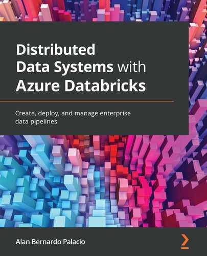
In Azure Databricks, we have also the option of using Structured Query Language (SQL) commands to import data from a CSV file into a temporary view that we can then query. We can do this by using %sql magic in a cell and loading the data in the CSV file into a temporary view, as follows:
%sql
CREATE TEMPORARY VIEW diamonds
USING CSV
OPTIONS (path "/databricks-datasets/Rdatasets/data-001/csv/ggplot2/diamonds.csv", header "true", mode "FAILFAST")
Pay attention to the fact that here, we pass the FAILFAST mode to stop the parsing of the file, causing an exception if faulty lines are found in it.
Once the data has been imported into the view, we can use SQL commands to perform queries on the temporary view, as follows:
%sql
SELECT * FROM diamonds
This will show us the temporary view that we just created, as illustrated in the following screenshot:
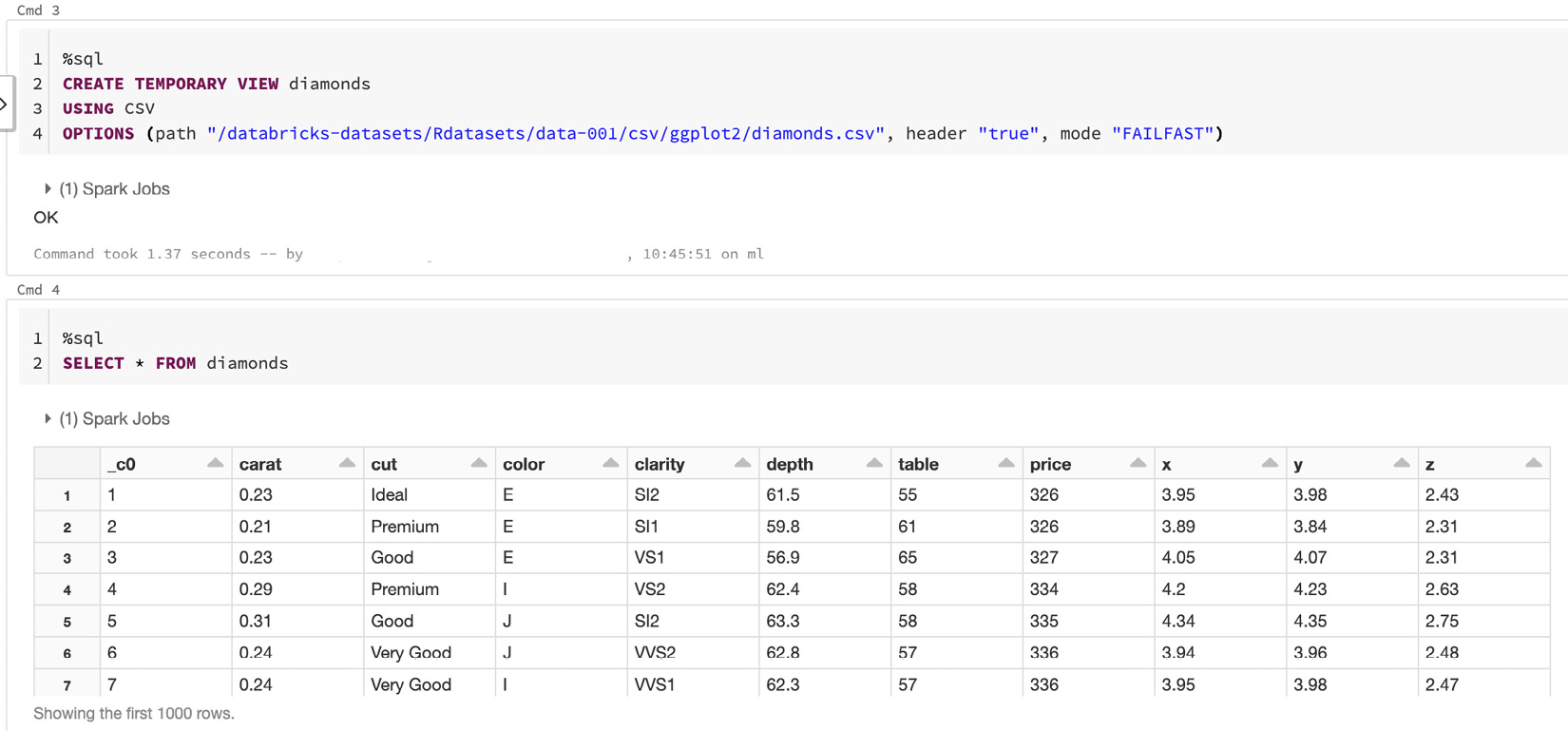
Figure 8.2 – Using SQL to read from a CSV file
If we read a CSV file specifying the schema, we may encounter some issues if the specified schema differs from what we have specified—for example, we may have a string value in a column that was specified as an integer data type. This could lead to results that differ considerably from the actual data. Therefore, it is always good practice to verify the correctness of the data.
We can specify the behavior of the CSV parser by selecting one of the available modes in which the parser runs. The available options for this mode are outlined here:
- PERMISSIVE: This is the default mode. Here, null values are inserted in fields that have not been parsed correctly. This allows us to inspect rows that have not been parsed correctly.
- DROPMALFORMED: This mode drops lines that hold values that could not be parsed correctly.
- FAILFAST: This mode aborts the reading of the file if any malformed data is found.
To set the mode, use the mode option, as illustrated in the following code snippet:
drop_wrong_schema = sqlContext.read.format("csv").option("mode", "FAILFAST")
In the next example, we will read a CSV file, specifying a known schema of the data with the parser mode set to drop malformed data if its type is not as specified. As discussed before, specifying the schema is always a good practice. If the schema of the data is already known, it is better to avoid schema inference. Here, we will read a file with columns for ID, name, and last name, the first as an integer and the rest as strings:
from pyspark.sql.types import StructType, StructField
from pyspark.sql.types import DoubleType, IntegerType, StringType
data_schema = StructType([
StructField("id", IntegerType()),
StructField("name", StringType()),
StructField("lastname", StringType())
])
(sqlContext
.read
.format("com.databricks.spark.csv")
.schema(data_schema)
.option("header", "true")
.option("mode", "DROPMALFORMED")
.load("some_input_file.csv"))
Now that we have gone through how to read tabular data from CSV files, we can use the data to extract features from it. These features will allow us to accurately model our data and have more effective machine learning and deep learning models. In the next section, we will learn how to perform feature engineering in Azure Databricks.
Feature engineering
Machine learning models are trained using input data to later provide as an outcome a prediction on unseen data. This input data is regularly composed of features that usually come in the form of structured columns. The algorithms use this data in order to infer patterns that may be used to infer the result. Here, the need for feature engineering arises with two main goals, as follows:
- Refactoring the input data to make it compatible with the machine learning algorithm we have selected for the task. For example, we need to encode categorical values if these are not supported by the algorithm we choose for our model.
- Improving the predictions produced by the models according to the performance metric we have selected for the problem at hand.
With feature engineering, we extract relevant features from the raw input data to be able to accurately represent it according to the way in which the problem to be solved has been modeled, resulting in an improvement in the performance model on novel data. It's good to keep in mind that the features used will influence the performance of the model more than everything else.
Feature engineering can be considered the process of transforming the input data into something that is easier to interpret for the machine learning algorithm by making key features or patterns more transparent, although we can sometimes generate new features to make the data visualization more interpretable or the pattern inference clearer for the model algorithm.
There are multiple strategies applied in feature engineering. Some of them are listed here:
- Missing data imputation and management
- Outlier handling
- Binning
- Logarithmic transformations
- One-hot encoding
- Normalization
- Grouping and aggregation operations
- Feature splitting
- Scaling
Some of these strategies have their application in just some algorithms or datasets, while others can be beneficial in all cases.
It is a common belief to think that the better the features you model, the better the performance you will achieve. While this is true in certain circumstances, it can also be misleading.
The performance of the model has many factors, with different degrees of importance. Among those factors are the selection of the algorithm, the available data, and the features extracted. You can also add to those factors the way in which the problem is modeled, and the objective metrics used to estimate performance. Nevertheless, great features are needed to effectively describe the structures inherent in your data and will make the job of the algorithm easier.
When working with large amounts of data, tools such as Spark SQL and MLlib can be very effective when used in feature engineering. Some third-party libraries are also included in Databricks Runtime ML, such as scikit-learn, which provides useful methods to extract features from data.
This section does not intend to go too deep into the mechanics of each algorithm, although some concepts will be reinforced to understand how they are applied in Azure Databricks.
Tokenizer
Tokenization can be generally described as a process in which we transform a string of input characters into an array formed by the individual sections that form it. These sections are called tokens and are generally individual words, but can be a certain number of characters, or a combination of words called n-grams. We will use these resulting tokens later on for some other form of processing to extract or transform features. In this sense, the tokenization process can be considered a task of feature engineering. The tokens are identified based on the specific modes that are passed to the parser.
In PySpark, we can use the simple Tokenizer class to tokenize a sequence of string inputs. The following code example shows how we can split sentences into sequences of words:
from pyspark.ml.feature import Tokenizer
sentenceDataFrame = sqlContext.createDataFrame([
(0, "Spark is great for Data Science"),
(0, "Also for data engineering"),
(1, "Logistic regression models are neat")
], ["label", "sentence"])
tokenizer = Tokenizer(inputCol="sentence", outputCol="words")
wordsDataFrame = tokenizer.transform(sentenceDataFrame)
for words_label in wordsDataFrame.select("words", "label").take(3):
print(words_label)
Here, we can see the encoded tokens:

Figure 8.3 – Output of the word tokenization
We can also use the more advanced RegexTokenizer tokenizer to specify token boundaries using regular expressions.
Binarizer
Binarization is a process in which you establish a numerical threshold on your features in order to transform them into binary features. Binarization is really useful to preprocess input data that holds continuous numerical features if you can assume that our data has a probabilistic normal distribution. This process makes the data easier to handle for the algorithms used in machine learning and deep learning because they describe the data into a more defined structure.
In PySpark, we can use the simple Binarizer class, which allows us to binarize continuous numerical features. Besides the common parameters of inputCol and outputCol, the simple Binarizer class has a parameter threshold that is used to establish the threshold to binarize the continuous numerical features. The features greater than this threshold are binarized to 1.0, and the ones equal or less than this threshold are binarized to 0.0. The following code example shows how we can use the Binarizer class to binarize numerical features. First, we import the Binarizer class and create an example DataFrame with label and feature columns:
from pyspark.ml.feature import Binarizer
continuousDataFrame = sqlContext.createDataFrame([
(0, 0.345),
(1, 0.826),
(2, 0.142)
], ["label", "feature"])
Next, we instantiate the Binarizer class, specifying a threshold and the input and output columns. Then, we transform the example DataFrame and store and display the results. The code to do this is illustrated in the following snippet:
binarizer = Binarizer(threshold=0.5, inputCol="feature",
outputCol="binarized_feature")
binarizedDataFrame = binarizer.transform(continuousDataFrame)
binarizedFeatures = binarizedDataFrame.select("binarized_feature")
for binarized_feature, in binarizedFeatures.collect():
print(binarized_feature)
We should see printed the binarized features of the transformed DataFrame according to the threshold that we have established. Next, we will learn how to apply a polynomial expansion to express features in a higher dimensional space.
Polynomial expansion
In mathematics, a polynomial expansion is a mathematical operation used to express a feature as a product of other higher-level features. Therefore, it can be used to expand features passed to express them as a set of features in a higher dimension.
A polynomial expansion can be considered a process of expanding your features into a polynomial space, in order to try to find patterns in that expanded space that otherwise might be difficult to find in a lower-dimension space. This is common when dealing with algorithms that make simple assumptions, such as linear regression, that might otherwise be unable to capture relevant patterns. This polynomial space in which we transform our features is formed by an n-degree combination of original dimensions. The PySpark PolynomialExpansion class provides us with this functionality. The following code example shows how you can use it to expand your features into a 3-degree polynomial space:
from pyspark.ml.feature import PolynomialExpansion
from pyspark.ml.linalg import Vectors
df = spark.createDataFrame([
(Vectors.dense([2.0, 1.0]),),
(Vectors.dense([0.0, 0.0]),),
(Vectors.dense([3.0, -1.0]),)
], ["features"])
polyExpansion = PolynomialExpansion(degree=3, inputCol="features", outputCol="polyFeatures")
polyDF = polyExpansion.transform(df)
polyDF.show(truncate=False)
Here, we can see the variables that were created in the polynomial expansion:

Figure 8.4 – Output features of the polynomial expansion
Having our features transformed into a higher-dimension space is a great tool to use in feature engineering. It allows us to describe data in different terms and increase the sensitivity of the machine learning algorithm to more complex patterns that might be hidden in the data.
StringIndexer
The PySpark StringIndexer class encodes a string column of labels into a column of labeled indices. These indices are in the range from 0 to numLabels, ordered by label frequencies. Therefore, the most frequent label will be indexed as 0. If the input column is numeric, the PySpark StringIndexer class will cast it to a string and index the string values.
The StringIndexer class takes an input column name and an output column name. Here, we will show how we can use it to index a column named cluster:
from pyspark.ml.feature import StringIndexer
df = sqlContext.createDataFrame(
[(0, "a"), (1, "b"), (2, "c"), (3, "a"),
(4, "a"), (5, "c")],
["id", "cluster"])
indexer = StringIndexer(inputCol="cluster",
outputCol="categoryIndex")
indexed = indexer.fit(df).transform(df)
indexed.show()
In the following screenshot, we can see that the strings were correctly indexed into a DataFrame of variables:

Figure 8.5 – Output transformation of the StringIndexer class
In this example, the a cluster gets index 0 because it is the most frequent, followed by c with index 1 and b with index 2.
One-hot encoding
One-hot encoding is a transformation used in feature engineering to create a group of binary values (often called dummy variables) that are mostly used to represent categorical variables with multiple possible values as variables with just a single high value (1) and all others a low value (0). Each of these Boolean features represents a single possible value in the original categorical variable.
One-hot encoding is sometimes used either for visualization, model efficiency, or to prepare your data according to the requirements of the training algorithms. For this, we construct different features by encoding the categorical variables. Instead of a single feature column with several levels, we split this column into Boolean features for each level, where the only accepted values are either 1 or 0.
One-hot encoding is a technique that is especially popular with neural networks and other algorithms in deep learning, to encode categorical features allowing algorithms that expect continuous features, such as logistic regression, to use these categorical features. In PySpark and Azure Databricks, we can use the OneHotEncoder class to map a column of label indices to an encoded column of binary vectors, with at most a single possible value. Here, we use the OneHotEncoder class to convert categorical features into numerical ones:
from pyspark.ml.feature import OneHotEncoder
df = spark.createDataFrame([
(0.0, 1.0),
(1.0, 0.0),
(2.0, 1.0),
(0.0, 2.0),
(0.0, 1.0),
(2.0, 0.0)
], ["clusterV1", "clusterV2"])
encoder = OneHotEncoder(inputCols=["clusterV1",
"clusterV2"],
outputCols=["catV1", "vatV2"])
model = encoder.fit(df)
encoded = model.transform(df)
encoded.show()
Here, we see the encoded variables that we obtained:
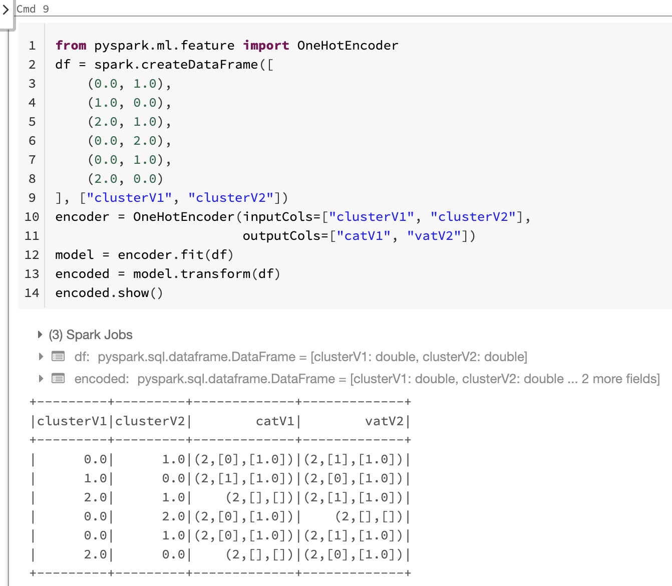
Figure 8.6 – Output of the one-hot encoding
In this way, we can use one-hot encoding to transform categorical features in one or many columns of a Spark DataFrame into numerical features that can be later transformed or directly passed to our model to train and infer.
VectorIndexer
In Azure Databricks, we can use the VectorIndexer class to index categorical features as an alternative to one-hot encoding. This class is used in data frames that contain columns of type Vector. It works by deciding which features are categorical and converts those features' original values into categorical indexes. The steps that it follows are outlined next:
- It takes as an input a column of type Vector and a maxCategories parameter, which—as the name suggests—specifies the threshold of a maximum number of categories for a single variable.
- It decides which features are categorical, based on the number of distinct values that they hold. The features with at most maxCategories will be marked as categorical.
- It computes 0-based category indices for each feature that was declared as categorical.
- Finally, it indexes the categorical features by transforming the original feature values into indices.
This indexing of categorical features allows us to overcome the limitations of certain algorithms such as Decision Trees and Tree Ensembles regarding handling categorical features to improve performance or to simply be able to use algorithms that allow just numerical features.
In the following code example, we will read an example dataset of labeled points and use the PySpark VectorIndexer class to decide which of the features that compose the dataset should be treated as categorical variables. We will later transform the values of those categorical features into indices:
from pyspark.ml.feature import VectorIndexer
from pyspark.mllib.util import MLUtils
data = MLUtils.loadLibSVMFile(sc, "data/mllib/sample_libsvm_data.txt").toDF()
indexer = VectorIndexer(inputCol="features",
outputCol="indexed",
maxCategories=10)
indexerModel = indexer.fit(data)
# Create new column "indexed" with categorical values transformed to indices
indexedData = indexerModel.transform(data)
This categorical data transformed into continuous can be then be passed to algorithms such as DecisionTreeRegressor in order to be able to handle categorical features.
Normalizer
Another common feature engineering method is to bring the data into a given interval. A first reason to do this is to limit the computations on a fixed range of values to prevent numerical inaccuracies and limit the computational power required that might arise when dealing with numbers that are either too big or too small. A second reason to normalize the numerical values of a feature is that some machine learning algorithms will handle data better when it has been normalized. There are several approaches that we can take in order to normalize our data.
These different approaches are due to some machine learning algorithms requiring different normalization strategies in order to perform efficiently. For example, in the case of k-nearest neighbors (KNN), the range of values in a particular feature impacts the weight of that feature in the model. Therefore, the bigger the values, the more importance the feature will have. In the case of the neural networks, this normalization might not impact the final performance results per se, but it will speed up the training and will avoid the exploiting and vanishing gradient problem that is caused because of the propagation of values that are either too big or too small to subsequent layers in the model. On the other hand, the decision tree-based machine learning algorithms neither benefit nor get hurt by the normalization.
The right normalization strategy will depend on the problem and selected algorithm, rather than some general statistical or computational considerations, and the right selection will always be closely tied to the domain knowledge.
In PySpark, the Normalizer class is a Transformer that transforms a dataset of Vector rows, normalizing each Vector to have the norm of the vector transformed into a unit. It takes as a parameter the value p, which specifies the p-norm used for normalization. This p value is set to 2 by default, which is equal to saying that we are transforming into the Euclidean norm.
The following code example demonstrates how to load a dataset in libsvm format and then normalize each row to have a unit norm:
from pyspark.mllib.util import MLUtils
from pyspark.ml.feature import Normalizer
data = MLUtils.loadLibSVMFile(sc, "data/mllib/sample_libsvm_data.txt")
dataFrame = sqlContext.createDataFrame(data)
# Normalize each Vector using $L^1$ norm.
normalizer = Normalizer(inputCol="features",
outputCol="normFeatures", p=1.0)
l1NormData = normalizer.transform(dataFrame)
# Normalize each Vector using $L^infty$ norm.
lInfNormData = normalizer.transform(dataFrame, {normalizer.p: float("inf")})
This normalization process is widely used in feature engineering and will help us to standardize the data and improve the behavior of learning algorithms.
StandardScaler
In many areas of nature, things tend to be governed by normal or Gaussian probabilistic distribution. Normalization is what we call in feature engineering the process of subtracting the mean value of a feature, which allows us to center our feature around 0. Then, we divide this by the standard deviation, which will tell us about the spread of our feature around 0. Finally, we will obtain a variable that is centered at 0, with a range of values between -1 and 1.
In Azure Databricks, we can use the PySpark StandardScaler class to transform a dataset of Vector rows into normalized features that have unit standard deviation and or 0 mean. It takes the following parameters:
- withStd: This parameter is set to true by default. It scales the data to unit standard deviation, which means that we divide by the standard deviation.
- withMean: This parameter is set to false by default. It will center the data with mean equal to 0 before scaling. It creates a dense output, so this will not work on sparse input and will raise an exception.
The PySpark StandardScaler class is a transformation that can be fit on a dataset to produce a StandardScalerModel; this latter model can, later on, be used to compute summary statistics on the input data. The StandardScalerModel can then be transformed into a column Vector in a dataset with unit standard deviation and/or 0 mean features.
Taking into account that if the standard deviation of a feature is already 0, StandardScalerModel will return as default 0.0 as the value in the Vector for that feature.
In the following code example, we will show how we can load a dataset that is in libsvm format and then normalize each feature to have a unit standard deviation.
- First, we will make the necessary imports and read the dataset, which is an example dataset in the mllib folder:
from pyspark.mllib.util import MLUtils
from pyspark.ml.feature import StandardScaler
data = MLUtils.loadLibSVMFile(sc, "data/mllib/sample_libsvm_data.txt")
dataFrame = sqlContext.createDataFrame(data)
scaler = StandardScaler(inputCol="features",
outputCol="scaledFeatures",
withStd=True, withMean=False)
- Then, we can compute summary statistics by fitting the StandardScaler class to the DataFrame created from the input data, as follows:
scalerModel = scaler.fit(dataFrame)
- Finally, we can normalize each feature to have a unit standard deviation, as follows:
scaledData = scalerModel.transform(dataFrame)
Normalization is widely used in data science. It helps us put all continuous numerical values on the same scale and can help us overcome numerous problems that arise when the continuous variables used in our learning algorithms are not bounded to fixed ranges and are not being centered.
Bucketizer
The PySpark Bucketizer class will transform a column of continuous features into a column of feature buckets, where these buckets are specified by users using the splits parameter:
The splits parameter is used for mapping continuous features into buckets. Specifying n+1 splits will yield n buckets. A bucket which is defined by splits x and y will hold values in the range [x,y) except for the last bucket, which will also include values in the range of y. These splits have to be strictly increasing. Keep in mind that otherwise specified, values outside the splits specified will be treated as errors. Examples of splits can be seen in the following code snippet:
splits = Array(Double.NegativeInfinity, 0.0, 1.0,
Double.PositiveInfinity)
splits = Array(0.0, 1.0, 2.0)
The split values must be explicitly provided to cover all Double values.
Take into account that if you don't know which are the upper bounds and lower bounds of the targeted column, it is best practice to add Double.NegativeInfinity and Double.PositiveInfinity as the bounds of your splits to prevent any potential error that might arise because of an "out of Bucketizer bounds " exception. Note also that these splits have to be specified in strictly increasing order.
In the following example, we will show how you can bucketize a column of Double values into another index-wised column using the PySpark Bucketizer class:
- First, we will make the necessary imports and define the DataFrame to be bucketized, as follows:
from pyspark.ml.feature import Bucketizer
splits = [-float("inf"), -0.5, 0.0, 0.5, float("inf")]
data = [(-0.5,), (-0.3,), (0.0,), (0.2,)]
dataFrame = sqlContext.createDataFrame(data,
["features"])
bucketizer = Bucketizer(splits=splits,
inputCol="features",
outputCol="bucketedFeatures")
- Then, we can transform the original data into its bucket index, as follows:
bucketedData = bucketizer.transform(dataFrame)
display(bucketedData)
- This is the obtained bucketized data:

Figure 8.7 – Bucketizer output features
- In PySpark, we can also use the QuantileDiscretizer class over Bucketizer where QuantileDiscretizer is an estimator that is able to handle Not a Number (NaN) values, and this is where the difference lies between the two of them, because the Bucketizer class is a transformer that raises an error if the input data holds NaN values. The following code snippet provides an example of a situation in which both classes yield similar outputs:
from pyspark.ml.feature import QuantileDiscretizer
from pyspark.ml.feature import Bucketizer
data = [(0, 18.0), (1, 19.0), (2, 8.0), (3, 5.0), (4, 2.2)]
df = spark.createDataFrame(data, ["id", "hour"])
result_discretizer = QuantileDiscretizer(numBuckets=3,
inputCol="hour",
outputCol="result").fit(df).transform(df)
result_discretizer.show()
splits = [-float("inf"),3, 10, float("inf")]
result_bucketizer = Bucketizer(splits=splits,
inputCol="hour",
outputCol="result").transform(df)
result_bucketizer.show()
Here the QuantileDiscretizer class will determine the bucket splits based on the data, while the Bucketizer class will arrange the data into buckets based on what you have specified via splits.
Therefore, it is better to use Bucketizer when you already have knowledge of which buckets you expect, while the QuantileDiscretizer class will estimate the splits for you.
In the preceding example, the outputs of both processes are similar because of the input data and the splits selected. Otherwise, results may vary significantly in different scenarios.
Element-wise product
An element-wise product is a mathematical operation very commonly used in feature engineering when working with data that is arranged as a matrix. The PySpark ElementwiseProduct class will multiply each input vector by a previously specified weight vector. To do this, it will use an element-wise multiplication that will scale each column of the input vector by a scalar multiplier defined as the weight.
The ElementwiseProduct class takes scalingVec as the main parameter, which is the transforming vector of this operation.
The following example will exemplify how we can transform vectors using the ElementwiseProduct class and a transforming vector value:
from pyspark.mllib.linalg.distributed import RowMatrix
v1 = sc.parallelize([[2.0, 2.0, 2.0], [3.0, 3.0, 3.0]])
mat = RowMatrix(v1)
v2 = Vectors.dense([0.0, 1.0, 2.0])
transformer = ElementwiseProduct(v2)
transformedData = transformer.transform(mat.rows)
print transformedData.collect()
This operation can then be understood as the Hadamard product, which is also known as the element-wise product between the input array and the weight vector, which in turn will give as a result another vector.
Time-series data sources
In data science and engineering, one of the most common challenges is temporal data manipulation. Datasets that hold geospatial or transactional data, which mostly lie in the financial and economics area of an application, are some of the most common examples of data that is indexed by a timestamp. Working in areas such as finance, fraud, or even socio-economic temporal data ultimately leads to the need to join, aggregate, and visualize data points.
This temporal data regularly comes in datetime formats that might vary not only in the format itself but in the information that it holds. One of the examples of this is the difference between the DD/MM/YYYY and MM/DD/YYYY format. Misunderstanding these different datetime formats could lead to failures or wrongly formed results if the formats used don't match up. Moreover, this data doesn't come in numerical format, which—as we have seen in previous sections of the chapter—can lead to several impediments that need to be overcome, one of them being the fact that this data cannot be interpreted easily by most of the learning algorithms used in machine and deep learning.
This is where feature engineering comes into play, providing us with the tools to transform and create new features from this data. An example of this could be to reorganize the data in numerical features such as day, month, and year, and even manipulate features using techniques as dynamic time warping to compare time series of different lengths, as could be the case when comparing the sales of the months of February and March, which have 28 and 31 days respectively.
In Azure Databricks, we have several functionalities in place that allow us to perform operations such as joins, aggregations, and windowing of time series, with the added benefit of doing this processing in parallel. Moreover, the Koalas API allows us to work with this data using a Pandas-like syntax that makes the transition from experiment to production much easier to handle.
In this example, we will work with financial data to illustrate how we can manipulate temporal datasets in Azure Databricks. The data that we will use is an example that is based on the stock market and holds trade information for different companies that are being traded. You can find more information about this kind of data at this link: https://www.tickdata.com/product/nbbo/:
- We can get example data by running the following code in an Azure notebook cell. This will download the data that we will read afterward:
%sh
wget https://pages.databricks.com/rs/094-YMS-629/images/ASOF_Quotes.csv ;
wget https://pages.databricks.com/rs/094-YMS-629/images/ASOF_Trades.csv ;
Here, we have downloaded two kinds of datasets, one for trades and one for offers. We will merge this data afterward over the time column to compare the trades and quotes made at the same points in time.
- Before reading the data, we will define a schema for it because this information is already known to us. We will assign the PySpark TimestampType class to the columns that hold temporal data about the trade execution and quote time. We will also rename the trade and execution time column names to events_ts to finally convert this data into Delta format. The code to do this is shown in the following snippet:
from pyspark.sql.types import *
trade_schema = StructType([
StructField("symbol", StringType()),
StructField("event_ts", TimestampType()),
StructField("trade_dt", StringType()),
StructField("trade_pr", DoubleType())
])
quote_schema = StructType([
StructField("symbol", StringType()),
StructField("event_ts", TimestampType()),
StructField("trade_dt", StringType()),
StructField("bid_pr", DoubleType()),
StructField("ask_pr", DoubleType())
])
Once we have downloaded the data and specified the desired schema for our Spark data frame, we can parse the CSV files according to the data schema and store them as Delta tables that we will be able to query afterward.
- We have decided to use Delta tables to benefit from the optimized data format that allows us to work with large compressed flat files and harness the power of the underlying engine, enabling us to easily scale and parallelize the process according to the amount of data available. The code is illustrated in the following snippet:
spark.read.format("csv").schema(trade_schema).option("header", "true").option("delimiter", ",").load("/tmp/finserv/ASOF_Trades.csv").write.mode('overwrite').format("delta").save('/tmp/finserv/delta/trades')
spark.read.format("csv").schema(quote_schema).option("header", "true").option("delimiter", ",").load("/tmp/finserv/ASOF_Quotes.csv").write.mode('overwrite').format("delta").save('/tmp/finserv/delta/quotes')
- After we have read and stored the data into the Delta tables, we can check that the data has been parsed correctly by displaying the resulting Delta table as a Spark Data Frame, as follows:
display(spark.read.format("delta").load("/tmp/finserv/delta/trades"))
Now that we have our transactional data available, we can use it to merge the trades and quotes, aggregate the trades, and perform windowing operations on it.
Joining time-series data
When working with time-series data, an as-of join is a merge technique that commonly refers to obtaining the value of a given event in the exact moment of the timestamp. For most of this temporal data, different types of datetime series will be joined together. In our particular case, we want to know for each company in the dataset the particular state of trade at any given point in time that we have available. Here, these states can be—for example—the NBBO, which is an acronym for National Best Bid Offer in trading and investing.
In the following example, we will obtain the state of the NBBO for each company available in the dataset. We will work the data in order to have for each company the state of the latest bid and offer for each of the data points that we have as timestamps. Once we have this computed, we can visualize the difference between bids and offers to comprehend at which points in time the liquidity of the company may hit a low point:
- First, we will merge the data on the symbol. We assume that we have already loaded the Delta tables into two Spark data frames named trades and offers, which we will merge on the symbol column. The code is shown in the following snippet:
un= trades.filter(col("symbol") == "K").select('event_ts', 'price', 'symbol', 'bid', 'offer', 'ind_cd').union(quotes.filter(col("symbol") == "K").select('event_ts', 'price', 'symbol', 'bid', 'offer', 'ind_cd'))
- After we have performed the merge, we can visualize the results, as follows:
display(un)
- Now that our data has been merged into a single Spark DataFrame, we can perform the windowing operation. First, we need to define the windowing function that we will use. To do this, we will use the Window class, which is a built-in method in PySpark to perform windowing operations. In the following code snippet, we will define the partition by the symbol column, which represents the company:
from pyspark.sql.window import Window
partition_spec = Window.partitionBy('symbol')
- Then, we need to specify the mechanism that will be used to sort the data. Here, we use the ind_cd column as the sort key, which is the column that specifies the values of the quotes before trades:
join_spec = partition_spec.orderBy('event_ts').
rowsBetween(Window.unboundedPreceding,
Window.currentRow)
- Then, we will use SQL commands to query the data and get the lasted_bid value by running a SELECT operation over the last bid and over join_spec, as follows:
%sql
select(last("bid", True).over(join_spec).alias("latest_bid"))
This way, we have demonstrated how easy is to manipulate time-series data in Azure Databricks using the PySpark API to run joins, merges, and aggregations on temporal data. In the next section, we will learn how we can leverage the benefit of the Pandas-like syntax to ease the transition from notebooks to production easier.
Using the Koalas API
When working with time series, it is fairly common to perform tasks related to imputation and removing duplicates. These duplicated records tend to happen when multiple records are inserted with high frequency on the dataset. We can use the Koalas API to perform these operations using a very familiar Pandas-like syntax, as was explored in previous chapters:
- In the following code example, we will read our Delta table into a Koalas DataFrame and perform deduplication by grouping by the event_ts column and then retrieve the maximum value for that point in time:
import databricks.koalas as ks
kdf_src = ks.read_delta("/tmp/finserv/delta/ofi_quotes2")
grouped_kdf = kdf_src.groupby(['event_ts'],
as_index=False).max()
grouped_kdf.sort_values(by=['event_ts'])
grouped_kdf.head()
- Now that we have removed the duplicates from our DataFrame, we can perform a shift in the data to create a lagged Koalas Data Frame that will be really helpful to do calculations such as moving average or other statistical trend calculations. As shown in the following code snippet, Koalas makes it easy to get lag or lead values within a window by using the shift method of the Koalas Data Frame:
grouped_kdf.set_index('event_ts', inplace=True,
drop=True)
lag_grouped_kdf = grouped_kdf.shift(periods=1,
fill_value=0)
lag_grouped_kdf.head()
- Now that we have lag values computed, we are to be able to merge this dataset with our original DataFrame to have all the data consolidated into a single structure to ease the calculation of statistical trends. In the following code example, we demonstrate how simple it is to merge two different data frames into a single one:
lagged = grouped_kdf.merge(lag_grouped_kdf,
left_index=True,
right_index=True,
suffixes=['', '_lag'])
lagged.head()
The Koalas API is very helpful for modeling our data and makes it easy to perform the necessary transformations, even when working with the time-series data. In the next section, we will learn how we can deal with possible missing values in our data frames when working in Azure Databricks.
Handling missing values
Real-life data is far from perfect, and cases of having missing values are really common. The mechanisms in which the data has become unavailable are really important to come up with a good imputation strategy. We call imputation the process in which we deal with values that are missing in our data, which in most contexts are represented as NaN values. One of the most important aspects of this is to know which values are missing:
- In the following code example, we will show how we can find out which columns have missing or null values by summing up all the Boolean output of the Spark isNull method by casting this Boolean output to integers:
from pyspark.sql.functions import col, sum df.select(*(sum(col(c).isNull().cast("int")).alias(c) for c in df.columns)).show()
- Another alternative would be to use the output of the Spark data frame describe method to filter out the count of missing values in each column and, finally, subtracting the count of rows to get the actual number of missing values, as follows:
from pyspark.sql.functions import lit
rows = df.count()
summary = df.describe().filter(col("summary") == "count") summary.select(*((lit(rows)-col(c)).alias(c) for c in df.columns)).show()
- Once we have identified the null values, we can use remove all rows that contain null values by using the na.drop() method of Spark data frames, as follows:
null_df.na.drop().show()
- We can also specify that the rows that have a number of null values greater than 2 be dropped, as follows:
null_df.na.drop(thresh=2).show()
- One of the other available options is to use the how argument of this method. For example, we can specify this parameter as any, which indicates to drop rows having any number of null values, as illustrated in the following code snippet:
null_df.na.drop(how='any').show()
- We can also drop null values on a single column using a subset parameter, which accepts list of column names, as illustrated in the following code snippet:
null_df.na.drop(subset=['Sales']).show()
- For example, we can specify to drop records that have null values in all of the specified subset of columns, as follows:
null_df.na.drop(how='all',subset=['Name','Sales']).show()
As mentioned before, one of the available options when dealing with missing data is to perform an imputation of them, which can be understood as filling those null values according to a predefined strategy that we know won't change the actual distribution of the data. It is always better to impute the null values rather than drop data.
- For example, we can choose to fill the null values with a string that helps us to identify them, as follows:
null_df.na.fill('NA').show()
- Or, we can also fill the missing values with an integer value, like this:
null_df.na.fill(0).show()
One more common option is filling the missing values with the mean or the median calculated from the present values. This way, we try to preserve the actual distribution of the data and try to not seriously affect other calculations such as the column mean. Nevertheless, it is necessary to keep in mind that if we do a new calculation of the mean, we will get another value.
- Here, we can fill a numeric column with the mean of the average for that particular column, as follows:
from pyspark.sql.functions import mean
mean_val=null_df.select(mean(null_df.Sales)).collect()
print(type(mean_val)) #mean_val is a list row object
print('mean value of Sales', mean_val[0][0])
mean_sales=mean_val[0][0]
- Now that we have calculated the mean value and stored it as a variable named men_sales, we can use this value to fill the null values in the sales column, as follows:
null_df.na.fill(mean_sales,subset=['Sales']).show()
In this way, we can handle all possible null or missing values that we find in the data, although the strategy that will be used to handle them depends greatly on the mechanism that created the missing values and the domain knowledge of the problem.
Extracting features from text
Extracting information from text relies on being able to capture the underlying language structure. This means that we intend to capture the meaning and relationship among tokens and the meaning they try to convey within a sentence. These sorts of manipulations and tasks associated with understanding the meaning in text yield a whole branch of an interdisciplinary field called natural language processing (NLP). Here, we will focus on some examples related to transforming text into numerical features that can be used later on the machine learning and deep learning algorithms using the PySpark API in Azure Databricks.
TF-IDF
Term Frequency-Inverse Document Frequency (TF-IDF) is a very commonly used text preprocessing operation to convert sentences into features created based on the relative frequency of the tokens that compose them. The term frequency-inverse is used to create a set of numerical features that are constructed based on how relevant a word is to the context, not only to a document in a collection or corpus.
In Azure Databricks ML, TF-IDF is an operation that is done in two separate parts, the first being the TF (+hashing ), followed by the IDF:
- TF: HashingTF is a PySpark Transformer class that takes an array of terms and converts them into fixed-length feature vectors. In feature engineering, when we refer to a "set of terms", this might imply that we are referencing a bag of words (BOW). The algorithm combines TF counts with the hashing trick (sometimes called feature hashing), in order to do a fast and efficient vectorization of the features into vectors or matrices, for dimensionality reduction.
- IDF: IDF is a PySpark Estimator class that is fitted on a dataset and yields as a result an IDFModel. The IDFModel takes as input feature vectors, which in this case come from the HashingTF class, and scales each feature column. It will automatically lower weights applied on columns, depending on the frequency it appears on the corpus.
In the following example, we take as input an array of sentences. Each sentence will be split into tokens using the PySpark Tokenizer class, which will yield a BOW for each sentence:
- Later—and, as mentioned, in the following code block —we will apply the HashingTF class to reduce the dimensionality of the feature vector:
from pyspark.ml.feature import HashingTF, IDF, Tokenizer
sentenceData = sqlContext.createDataFrame([
(0, "Hi I heard about Spark"),
(0, "I wish Java could use case classes"),
(1, "Logistic regression models are neat")
], ["label", "sentence"])
tokenizer = Tokenizer(inputCol="sentence", outputCol="words")
wordsData = tokenizer.transform(sentenceData)
hashingTF = HashingTF(inputCol="words",
outputCol="rawFeatures",
numFeatures=20)
- Later, we will apply the IDF class to rescale the obtained features as a good practice when we use this in a machine learning or deep learning algorithm to avoid issues with gradients and generally improve the performance. The code for this is shown in the following snippet:
featurizedData = hashingTF.transform(wordsData)
idf = IDF(inputCol="rawFeatures",outputCol="features")
idfModel = idf.fit(featurizedData)
rescaledData = idfModel.transform(featurizedData)
- Finally, we can display the obtained features, as follows:
for features_label in rescaledData.select("features","label").take(3):
print(features_label)
- We can see the entire process of generating the variables, as shown in the following screenshot:

Figure 8.8 – Output features of the TF-IDF operation
In this way, we have our features extracted from the text and converted into scaled numerical features that can be fed into any learning algorithm.
Word2vec
Word2vec is an embedding technique that is used in feature engineering for NLP. It uses a neural network to learn the associations between words from a large corpus of text and it produces vectors that represent each token. This vector holds properties that allow us to indicate the semantic similarity between two words just by measuring the distance between the vectors that represent them, using (for example) cosine similarity. These vectors are often called word embeddings and they commonly have several hundreds of dimensions used to represent them.
In PySpark, Word2vec is an Estimator class that takes as input an array of and trains a Word2VecModel, which is a model that maps each word into a single fixed-sized vector.
In the code example shown next, we start with a set of documents, each of them represented as a sequence of words. For each document, we transform it into a feature vector. This feature vector could then be passed to a learning algorithm:
- In the following code example, we will create a Spark data frame with sentences that are split into their tokens using a simple split on the string, meaning that each row represents a BOW from that sentence:
from pyspark.ml.feature import Word2Vec
documentDF = sqlContext.createDataFrame([
("Hi I heard about Spark".split(" "), ),
("I wish Java could use case classes".split(" "), ),
("Logistic regression models are neat".split(" "), )
], ["text"])
- Then, we can map those arrays into vectors, as follows:
word2Vec = Word2Vec(vectorSize=3, minCount=0, inputCol="text", outputCol="result")
- Finally, we can fit the Word2Vec model to the array we just created and obtain the resulting features by transforming the input DataFrame using the fitted model, as follows:
model = word2Vec.fit(documentDF)
result = model.transform(documentDF)
for feature in result.select("result").take(3):
print(feature)
- We can see here the whole process executed on a single cell in an Azure Databricks notebook:

Figure 8.9 – Output embeddings using Word2Vec
In this way, we can very simply create a numerical representation obtained from text sources, using one of the most widely used models in text embeddings: Word2Vec.
Training machine learning models on tabular data
In this example, we will use a very popular dataset in data science, which is the wine dataset of physicochemical properties, to predict the quality of a specific wine. We will be using Azure Databricks Runtime ML, so be sure to attach the notebook to a cluster running this version of the available runtimes, as specified in the requirements at the beginning of the chapter.
Engineering the variables
We'll get started using the following steps:
- Our first step is to load the necessary data to train our models. We will load the datasets, which are stored as example datasets in DBFS, but you can also get them from the UCI Machine Learning repository. The code is shown in the following snippet:
import pandas as pd
white_wine = pd.read_csv("/dbfs/databricks-datasets/wine-quality/winequality-white.csv", sep=";")
red_wine = pd.read_csv("/dbfs/databricks-datasets/wine-quality/winequality-red.csv", sep=";")
- Next, we will merge these two pandas Data Frames into a single one, and add a new binary feature named is_red to distinguish between the two of them, as follows:
red_wine['is_red'] = 1
white_wine['is_red'] = 0
data = pd.concat([red_wine, white_wine], axis=0)
- After this, we will remove spaces from the column names in order to be able to save this as a Spark data frame, as follows:
data.rename(columns=lambda x: x.replace(' ', '_'), inplace=True)
data.head()
- Here, we can see the created Pandas Data frame:

Figure 8.10 – Renamed columns of the dataset
- Now that we have a unified dataset, we will create a new feature named high_quality for all the wines that have a quality above 7, as follows:
high_quality = (data.quality >= 7).astype(int)
data.quality = high_quality
- Afterward, we can split our dataset in train and test datasets, which we will use to train our machine learning model later on, inferring on the quality column. In the following code block, we import the scikit-learn train_test_split function in order to split the data into the features defined by X and the objective column defined as y:
from sklearn.model_selection import train_test_split
train, test = train_test_split(data, random_state=123)
X_train = train.drop(["quality"], axis=1)
X_test = test.drop(["quality"], axis=1)
y_train = train.quality
y_test = test.quality
As a result, we have the features and objective columns split into train and test datasets that can be used to train and benchmark the model.
Building the ML model
Here, we will use a classifier given the fact that what we are trying to predict is a binary output on a tabular dataset. The selected algorithm will be a Random Forest classifier available in the scikit-learn Python library. We will also make use of MLflow to keep track of the model performance, and to save the model for later use:
- We will start by doing all the necessary imports, as follows:
import mlflow
import mlflow.pyfunc
import mlflow.sklearn
import numpy as np
from sklearn.ensemble import RandomForestClassifier
from sklearn.metrics import roc_auc_score
from mlflow.models.signature import infer_signature
- We will create a wrapper class named SklearnModelWrapper around the model, inheriting from the mlflow.pyfunc.PythonModel class. This class will return the probability of an instance being part of a determined class. The code is shown in the following snippet:
class SklearnModelWrapper(mlflow.pyfunc.PythonModel):
def __init__(self, model):
self.model = model
def predict(self, context, model_input):
return self.model.predict_proba(model_input)[:,1]
- After we have defined our model, we will use mlflow.start_run to create a new MLflow run that will allow us to keep up with the track performance. We can also call mlflow.log_param to show which parameters are being passed to the model. In the following code example, mlflow.log_metric will be recording the performance metrics that we have selected, such as the receiver operating characteristic (ROC) in this case:
with mlflow.start_run(run_name='untuned_random_forest'):
n_estimators = 10
model = RandomForestClassifier(n_estimators=n_estimators, random_state=np.random.RandomState(123))
model.fit(X_train, y_train)
predictions_test = model.predict_proba(X_test)[:,1]
auc_score = roc_auc_score(y_test, predictions_test)
mlflow.log_param('n_estimators', n_estimators)
mlflow.log_metric('auc', auc_score)
wrappedModel = SklearnModelWrapper(model)
signature = infer_signature(X_train, wrappedModel.predict(None, X_train))
mlflow.pyfunc.log_model("random_forest_model", python_model=wrappedModel, signature=signature)
- In the preceding code snippet, the predict_proba function will return a tuple with the probability of belonging to one of the two classes. We will keep just one, so we slice the output with [:, 1. After the model has been deployed, we create a signature that will be used later on to validate inputs. Here, we can see the whole code being run on an Azure Databricks notebook:

Figure 8.11 – Fitting the model using the MLflow start_run decorator
- After the model has been trained, we can examine the learned feature importance output of the model as a sanity check, as follows:
feature_importances = pd.DataFrame(model.feature_importances_, index=X_train.columns.tolist(), columns=['importance'])
feature_importances.sort_values('importance', ascending=False)
- Here, we can see which variables were most important for the model:
Figure 8.12 – Model feature importance
- It shows that both alcohol and density are important in predicting quality. You can click on the Experiment button at the upper right to see the Experiment Runs sidebar, as illustrated in the following screenshot:
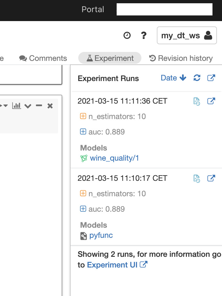
Figure 8.13 – Tracked experiment runs
In this example, this model achieved an area under the curve (AUC) of 0.889.
Registering the model in the MLflow Model Registry
The next steps will be to register the model that we just trained in the MLflow Model Registry, which is a centralized model registry that allows us to manage the full life cycle of a trained model and to use our model from anywhere in Azure Databricks. This model repository will not only store the models but will also provide us with versioning control of them, as well as allow us to add descriptions and comments:
- In the next example, we will show how we can register our model programmatically, but you can also do this by using the user interface (UI) in the Azure Databricks workspace. First, we will store the run ID of the latest run for the model that we just trained. We search for the run ID, filtering by the name of the model using the tags.mlflow.runName parameter, as follows:
run_id = mlflow.search_runs(filter_string='tags.mlflow.runName = "untuned_random_forest"').iloc[0].run_id
model_name = "wine_quality"
model_version = mlflow.register_model(f"runs:/{run_id}/random_forest_model", model_name)
If you navigate to the Models page in your Azure Databricks workspace, you will see the model we just registered.
- After our model has been successfully registered, we can set the stage of this model. We will move our model to production and load it in the notebook, as shown in the following code snippet:
from mlflow.tracking import MlflowClient
client = MlflowClient()
client.transition_model_version_stage(
name=model_name,
version=model_version.version,
stage="Production",
)
- We can see here in the cell output that the model was correctly registered:

Figure 8.14 – Correctly registered model
- Now, we can use our model by referencing using the f"models:/{model_name}/production" path. The model can then be loaded into a Spark user-defined function (UDF) so that it can be applied to the Delta table for batch inference. The following code will load our model and apply it to a Delta table:
import mlflow.pyfunc
from pyspark.sql.functions import struct
apply_model_udf = mlflow.pyfunc.spark_udf(spark, f"models:/{model_name}/production")
new_data = spark.read.format("delta").load(table_path)
- Once the model has been loaded and the data has been read from the Delta table, we can use a struct to pass the input variables to the model registered as a UDF, as follows:
udf_inputs = struct(*(X_train.columns.tolist()))
new_data = new_data.withColumn(
"prediction",
apply_model_udf(udf_inputs)
)
display(new_data)
Here, each record in the Delta table will have now an associated prediction.
Model serving
We can use our model for low-latency predictions by using the MLflow model serving to provide us with an endpoint so that we can issue requests using a REST API and get the predictions as a response.
You will need your Databricks token to be able to issue the request to the endpoint. As mentioned in previous chapters, you can get your token in the User Settings page in Azure Databricks.
Before being able to make requests to our endpoint, remember to enable the serving on the model page in the Azure Databricks workspace. You can see a reminder of how to do this in the following screenshot:

Figure 8.15 – Enabling model serving
- Finally, we can call our model. The following example function will issue a Pandas data frame and will return the inference for each row in the DataFrame:
import os
import requests
import pandas as pd
def score_model(dataset: pd.DataFrame):
url = 'https://YOUR_DATABRICKS_URL/model/wine_quality/Production/invocations'
headers = {'Authorization': f'Bearer {your_databricks_token}'
data_json = dataset.to_dict(orient='split')
response = requests.request(method='POST', headers=headers, url=url, json=data_json)
if response.status_code != 200:
raise Exception(f'Request failed with status {response.status_code}, {response.text}')
return response.json()
- We can compare the results we get on the local model by passing the X_test data, as shown in the following code snippet. We should obtain the same results:
num_predictions = 5
served_predictions = score_model(X_test[:num_predictions])
model_evaluations = model.predict(X_test[:num_predictions])
pd.DataFrame({
"Model Prediction": model_evaluations,
"Served Model Prediction": served_predictions,
})
This way, we have enabled low-latency predictions on smaller batches of data by using our published model as an endpoint to issue requests.
Summary
In this section, we have covered many examples related to how we can extract and improve features that we have available in the data, using methods such as tokenization, polynomial expansion, and one-hot encoding, among others. These methods allow us to prepare our variables for the training of our models and are considered as a part of feature engineering.
Next, we dived into how we can extract features from text using TF-IDF and Word2Vec and how we can handle missing data in Azure Databricks using the PySpark API. Finally, we have finished with an example of how we can train a deep learning model and have it ready for serving and get predictions when posting REST API requests.
In the next chapter, we will focus more on handling large amounts of data for deep learning using TFRecords and Petastorm, as well as on how we can leverage existing models to extract features from new data in Azure Databricks.