The typical data scientist consistently has a series of extremely complicated problems on their mind beyond considerations stemming from their system infrastructure. Still, it is inevitable that infrastructure issues will present themselves. To oversimplify, we might draw a distinction between the “modeling problem” and the “engineering problem.” The data scientist is uniquely qualified to solve the former, but can often come up short in solving the latter.
Docker has been widely adopted by the system administrator and DevOps community as a modern solution to the challenges presented in high availability and high performance computing.1 Docker is being used for the following: transitioning legacy applications to a more modern “microservice”-based approach, facilitating continuous integration and continuous deployment for the integration of new code, and optimizing infrastructure usage.
In this book, I discuss Docker as a tool for the data scientist, in particular in conjunction with the popular interactive programming platform Jupyter. Using Docker and Jupyter, the data scientist can easily take ownership of their system configuration and maintenance, prototype easily deployable and scalable data solutions, and trivially clone entire systems with an eye toward replicability and communication. In short, I propose that skill with Docker is just enough knowledge of systems operations to make the data scientist dangerous. Having done this, I propose that Docker can add high performance and availability tools to the data scientist’s toolbelt and fundamentally change the way that models are developed, prototyped, and scaled.
“Big Data”
A precise definition of “big data ” will elude even the most seasoned data wizard. I favor the idea that big data is the exact scope of data that is no longer manageable without explicit consideration to its scope. This will no doubt vary from individual to individual and from development team to development team. I believe that mastering the concepts and techniques associated with Docker presented herein will drastically increase the size and scope of what exactly big data is for any reader.
Recommended Practice for Learning
In this first chapter, you jump will headlong into using Docker and Jupyter on a cloud system. I hope that readers have a solid grasp of the Python numerical computing stack, although I believe that nearly anyone should be able to work their way through this book with enough curiosity and liberal Googling.
For the purposes of working through this book, I recommend using a sandbox system. If you are able to install Docker in an isolated, non-mission critical setting, you can work through this text without fear of “breaking things.” For this purpose, I here describe the process of setting up a minimal cloud-based system for running Docker using Amazon Web Services (AWS) .
As of the writing of this book, AWS is the dominant cloud-based service provider. I don’t endorse the idea that its dominance is a reason a priori to use its services. Rather, I present an AWS solution here as one that will be the easiest to adopt by the largest group of people. Furthermore, I believe that this method will generalize to other cloud-based offerings such as DigitalOcean2 or Google Cloud Platform,3 provided that the reader has secure shell (ssh) access to these systems and that they are running a Linux variant.
I present instructions for configuring a system using Elastic Compute Cloud (EC2) . New users receive 750 hours of free usage on their T2.micro platform and I believe that this should be more than enough for the typical reader’s journey through this text.
Over the next few pages, I outline the process of configuring an AWS EC2 system for the purposes of working through this text. This process consists of
Configuring a key pair
Creating a new security group
Creating a new EC2 instance
Configuring the new instance to use Docker
Set up a New AWS Account
To begin, set up an AWS account if you do not already have one.4
Note
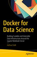
This work can be done in any region, although it is recommended that readers take note of which region they have selected for work (Figure 1-1). For reasons I have long forgotten, I choose to work in us-west-2.
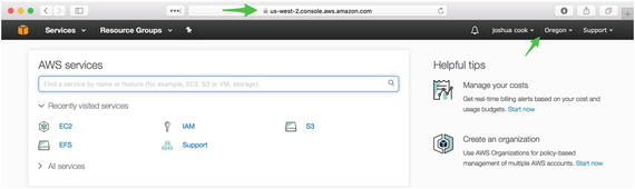
Figure 1-1. Readers should take note of the region in which they are working
Configure a Key Pair
In order to interface with your sandbox system running on AWS EC2, you will need an ssh key pair. Amazon EC2 uses public-key cryptography to facilitate all connections to running EC2 instances.5 In your case, this means the creation of a secure connection between your local system and a sandbox system you will configure on an EC2 instance. To do this, you will create an ssh key pair locally and import the public component of the key pair into AWS. When you create a new instance, you have AWS provision the new instance with the public key, so that you can use your local private key to connect to the instance.
Note
Windows users are encouraged to make use of the excellent Git BASH tool available as part of the Git for Windows package here: https://git-for-windows.github.io . Git BASH will include all of the necessary command line tools that you will be using, including ssh-keygen and ssh.
In Listing 1-1, you use the ssh-keygen tool to create a key pair on your local system. For these purposes (that is, a disposable sandbox AWS system), you can leave all fields blank, including a passphrase to use the ssh key. The location in which you save the key will vary from system to system. The default location on my system is ∼/.ssh/id_rsa where ∼ signifies the current user’s home directory.6 This process will create id_rsa and id_rsa.pub, a key pair. You will place the id_rsa.pub key into systems you wish to access and thus be able to ssh into these systems using the id_rsa file.
Listing 1-1. Create a New Key Pair
$ ssh-keygen -t rsaGenerating public/private rsa key pair.Enter file in which to save the key (/home/ubuntu/.ssh/id_rsa):Enter passphrase (empty for no passphrase):Enter same passphrase again:Your identification has been saved in /home/ubuntu/.ssh/id_rsa.Your public key has been saved in /home/ubuntu/.ssh/id_rsa.pub.The key fingerprint is:SHA256:g5IYNQMf1n1jW5p36Y9I/qSPxnckhT665KtiB06xu2U ubuntu@ip-172-31-43-19The key's randomart image is:+---[RSA 2048]----+| ..*. . || + +. . + . || . . o * o || o . .. + . + .|| . o . So . + . || . +. . = .|| o oE+.o.* || =o.o*+o o|| ..+.o**o. |+----[SHA256]-----+
In Listing 1-2, you verify that the contents of the key using the cat tool. You display a public key that was created on a remote Ubuntu system, as can be seen at the end of the key (ubuntu@ip-172-31-43-19). This should appear similar on any system.
Listing 1-2. Verify Newly Created ssh-key
$ cat ∼/.ssh/id_rsa.pubssh-rsa AAAAB3NzaC1yc2EAAAADAQABAAABAQDdnHPEiq1a4OsDDY+g9luWQS8pCjBmR64MmsrQ9MaIaE5shIcFB1Kg3pGwJpypiZjoSh9pS55S9LckNsBfn8Ff42ALLjR8y+WlJKVk/0DvDXgGVcCc0t/uTvxVx0bRruYxLW167J89UnxnJuRZDLeY9fDOfIzSR5eglhCWVqiOzB+OsLqR1W04Xz1oStID78UiY5msW+EFg25Hg1wepYMCJG/Zr43ByOYPGseUrbCqFBS1KlQnzfWRfEKHZbtEe6HbWwz1UDL2NrdFXxZAIXYYoCVtl4WXd/WjDwSjbMmtf3BqenVKZcP2DQ9/W+geIGGjvOTfUdsCHennYIEUfEEP ubuntu@ip-172-31-43-19
Create a New Key Pair on AWS
Log in to your AWS control panel and navigate to the EC2 Dashboard, as shown in Figure 1-2. First, access “Services” (Figure 1-2, #1) then access “EC2” (Figure 1-2, #2). The Services link can be accessed from any page in the AWS website.
Figure 1-2. Access the EC2 control panel
Once at the EC2 control panel, access the Key Pairs pane using either link (Figure 1-3).

Figure 1-3. Access key pairs in the EC2 Ddashboard
From the Key Pairs pane, choose “Import Key Pair.” This will activate a modal that you can use to create a new key pair associated with a region on your AWS account. Make sure to give the key pair a computer-friendly name, like from-MacBook-2017. Paste the contents of your public key (id_rsa.pub) into the public key contents. Prior to clicking Import, your key should appear as in Figure 1-4. Click Import to create the new key.
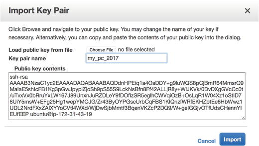
Figure 1-4. Import a new key pair
Note
Many AWS assets are created uniquely by region. Key pairs created in one region will not be available in another.
You have created a key pair between AWS and your local system. When you create a new instance, you will instruct AWS to provision the instance with this key pair and thus you will be able to access the cloud-based system from your local system.
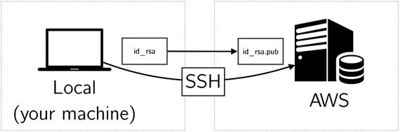
Figure 1-5. Connect to AWS from your local machine using an SSH key
Note
The terminology can be a bit confusing. AWS refers to an uploaded public key as a “key pair.” To be clear, you are uploading the public component of a key pair you have created on your system (e.g. id_rsa.pub). The private key will remain on your system (e.g. id_rsa).
Create a New Security Group
From the EC2 Dashboard, access the Security Group pane using either link (Figure 1-6).

Figure 1-6. Access security groups in the EC2 Dashboard
From the Security Group pane, click “Create Security Group.” Give the security group a computer friendly group name like jupyter_docker. Give the security group a description like “Open access to Jupyter and Docker default ports.” Use the default VPC. Access the Inbound tab and configure the following security rules:
SSH: Port Range: 22, Source: Anywhere
HTTP: Port Range: 80, Source: Anywhere
HTTPS: Port Range: 443, Source: Anywhere
Custom TCP Rule: Port Range: 2376, Source: Anywhere
Custom TCP Rule: Port Range: 8888, Source: Anywhere
When you have added all of these rules, it should appear as in Figure 1-7. Table 1-1 shows a list of ports and the services that will be accessible over these ports.
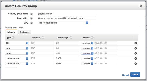
Figure 1-7. Inbound rules for new security group
Table 1-1. Ports and Usages
Port | Service Available |
|---|---|
22 | SSH |
80 | HTTP |
443 | HTTPS |
2376 | Docker Hub |
8888 | Jupyter |
Create a New EC2 Instance
To create a new instance, start from the EC2 Dashboard and click the Launch Instance button (Figure 1-8).
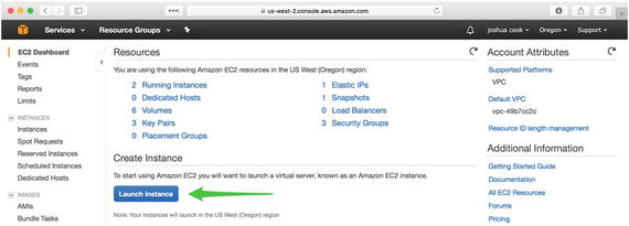
Figure 1-8. Launch a new instance
The launching of a new instance is a multi-step process that walks the user through all configurations necessary. The first tab is “Choose AMI.” An AMI is an Amazon Machine Image7 and contains the software you will need to run your sandbox machine. I recommend choosing the latest stable Ubuntu Server release that is free-tier eligible. At the time of writing, this was ami-efd0428f, Ubuntu Server 16.04 LTS (HVM), SSD Volume Type (Figure 1-9).
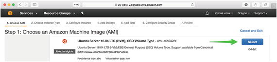
Figure 1-9. Choose the latest stable Ubuntu Server release as AMI
The second tab is “Choose Instance Type.” In usage, I have found that the free tier, t2.micro (Figure 1-10), is sufficient for many applications, especially the sort of sandbox-type work that might be done in working through this text. This is to say that while working through the text, you may not be doing extended work on datasets, but rather learning about how to configure different systems. As such, your memory needs may be diminished. The ultimate goal is for the reader to be able to create and destroy machines at will. At this level of mastery, the reader can choose the minimum requirements for any application.

Figure 1-10. Use the t2.micro type
The third tab, “Configure Instance,” can be safely ignored.
The fourth tab is “Add Storage.” This option is also specific to intended usage. It should be noted that Jupyter Docker images can take up more than 5GB of disk space in the local image cache. For this reason, it is recommended to raise the value from the default 8GB to somewhere in the neighborhood of 20GB.
The fifth tab, “Add Tags,” can be safely ignored.
The sixth tab, “Configure Security Group,” is critical for the proper functioning of your systems. Previously, you configured a new security group to be used by your system. You will need to assign the security group that you just created, jupyter_docker, to the instance you are configuring. Choose “Select an existing security group,” and then select the security group you just created. Verify that ports 22, 80, 443, 2376, and 8888 are available in the Inbound Rules at the bottom of the tab (Figure 1-11).
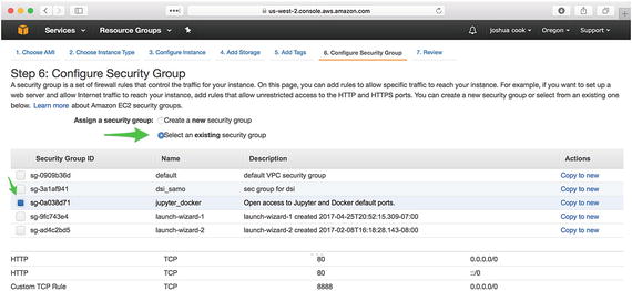
Figure 1-11. Configure the security group for all traffic
Note
Most readers will receive a warning from AWS at this final phase that says something to the effect of “Improve your instances' security. Your security group, jupyter_docker, is open to the world.” It is the opinion of this author that this warning can be safely ignored. The warning is letting us know that the instance we are preparing to launch can be accessed on the open web. This is intentional and by design. In this first and last conversation about system security, we will wave our hands at the concern and quickly move to the business of developing short-lifespan scalable systems.
Finally, click “Review and Launch.” Here, you see the specific configuration of the EC2 instance you will be creating. Verify that you are creating a t2.micro running the latest free tier-eligible version of Ubuntu Server and that it is available to all traffic, and then click the Launch button (Figure 1-12).
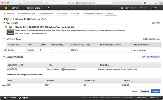
Figure 1-12. Launch the new EC2 instance
In a final confirmation step, you will see a modal titled “Select an existing key pair or create a new key pair.” Select the key pair you previously created. Check the box acknowledging access to that key pair and launch the instance (Figure 1-13).
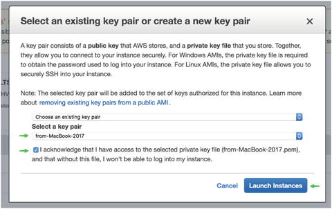
Figure 1-13. Select the key pair previously imported
You should see a notification that the instance is now running. Click the View Instances tab in the lower right corner to be taken to the EC2 Dashboard Instances pane, where you should see your new instance running.
Make note of the IP address of the new instance (Figure 1-14).

Figure 1-14. Note the IP address of a running instance
Configure the New EC2 Instance for Using Docker
Having set up an EC2 instance, you ssh into the instance using the IP you just obtained in order to provision the new instance with Docker (Listing 1-3).
Listing 1-3. SSH into EC2 Instance
$ ssh [email protected]Welcome to Ubuntu 16.04.2 LTS (GNU/Linux 4.4.0-64-generic x86_64)...
Note
The first time you access your EC2 instance, you should see the following message: The authenticity of host '54.244.109.176 (54.244.109.176)' can't be established ... Are you sure you want to continue connecting (yes/no)? This is expected. You should hit <ENTER> to accept or type yes and hit <ENTER>.
Next (Listing 1-4), you install and configure Docker using a convenient install script provided by the Docker team. The script is obtained from get.docker.com and passed via pipe (|) to a shell (sh).
Listing 1-4. Install Docker Via a Shell Script
$ curl -sSL https://get.docker.com/ | shapparmor is enabled in the kernel and apparmor utils were already installed+ sudo -E sh -c sleep 3; apt-get update...+ sudo -E sh -c docker versionClient:Version: 17.04.0-ceAPI version: 1.28Go version: go1.7.5Git commit: 4845c56Built: Mon Apr 3 18:07:42 2017OS/Arch: linux/amd64Server:Version: 17.04.0-ceAPI version: 1.28 (minimum version 1.12)Go version: go1.7.5Git commit: 4845c56Built: Mon Apr 3 18:07:42 2017OS/Arch: linux/amd64Experimental: false...
In Listing 1-5, you add the ubuntu user to the docker group. By default, the command line docker client will require sudo access in order to issue commands to the docker daemon. You can add the ubuntu user to the docker group in order to allow the ubuntu user to issue commands to docker without sudo.
Listing 1-5. Add the Ubuntu User to the Docker Group
$ sudo usermod -aG docker ubuntuFinally, in order to force the changes to take effect, you reboot the system (Listing 1-6). As an alternative to rebooting the system, users can simply disconnect and reconnect to their remote system.
Listing 1-6. Restart the Docker Daemon
$ sudo rebootThe reboot will have the effect of closing the secure shell to your EC2 instance. After waiting a few moments, reconnect to the system. At this point, your system will be ready for use. sudo should no longer be required to issue commands to the docker client. You can verify this by connecting to your remote system and checking the dock version (Listing 1-7).
Listing 1-7. Log into the Remote System and Check the Docker Version
$ ssh [email protected]$ docker -vDocker version 17.04.0-ce, build 4845c56
Infrastructure Limitations on Data
Before commencing with the nuts and bolts of using Docker and Jupyter to build scalable systems for computational programming, let’s conduct a simple series of experiments with this new AWS instance. You’ll begin with a series of simple questions:
What size dataset is too large for a t2.micro to load into memory?
What size dataset is so large that, on a t2.micro , it will prevent Jupyter from fitting different kinds of simple machine learning classification models 8 (e.g. a K Nearest Neighbor model)? A Decision Tree model? A Logistic Regression? A Support Vector Classifier?
To answer these questions, you will proceed in the following fashion:
Run the jupyter/scipy-notebook image using Docker on your AWS instance.
Monitor memory usage at runtime and as you load each dataset using docker stats.
Use the sklearn.datasets.make_classification function to create datasets of arbitrary sizes using a Jupyter Notebook and perform a fit.
Restart the Python kernel after each model is fit.
Take note of the dataset size that yields a memory exception.
Pull the jupyter/scipy-notebook image
Since you are working on a freshly provisioned AWS instance, you must begin by pulling the Docker image with which you wish to work, the jupyter/scipy-notebook. This can be done using the docker pull command, as shown in Listing 1-8. The image is pulled from Project Jupyter’s public Docker Hub account.9
Listing 1-8. Pull the jupyter/scipy-notebook image.
ubuntu@ip-172-31-6-246:∼$ docker pull jupyter/scipy-notebookUsing default tag: latestlatest: Pulling from jupyter/scipy-notebook693502eb7dfb: Pull completea3782c2efb41: Pull complete9cb32b776a40: Pull completee539f5722cd5: Pull completeb4690d4047c6: Pull complete121dc465f5c6: Pull completec352772bbcfd: Pull completeeeda14d1c421: Pull complete0057b9e76c8a: Pull completee63bd87d75dd: Pull complete055904fbc069: Pull completed336770b8a83: Pull completed61dbef85c7d: Pull completec1559927bbf2: Pull completeee5b638d15a3: Pull completedc937a931aca: Pull complete4327c0faf37c: Pull completeb37332c24e8c: Pull completeb230bdb41817: Pull complete765fecb84d9c: Pull complete97efa424ddfa: Pull completeccfb7ed42913: Pull complete2fb2abb673ce: Pull completeDigest: sha256:04ad7bdf5b9b7fe88c3d0f71b91fd5f71fb45277ff7729dbe7ae20160c7a56dfStatus: Downloaded newer image for jupyter/scipy-notebook:latest
Once you have pulled the image, it is now present in your docker images cache. Anytime you wish to run a new Jupyter container, Docker will load the container from the image in your cache.
Run the jupyter/scipy-notebook Image
In Listing 1-9, you run a Jupyter Notebook server using the minimum viable docker run command. Here, the -p flag serves to link port 8888 on the host machine, your EC2 instance, to the port 8888 on which the Jupyter Notebook server is running in the Docker container.
Listing 1-9. Run Jupyter Notebook Server
$ docker run -p 8888:8888 jupyter/scipy-notebook[I 22:10:01.236 NotebookApp] Writing notebook server cookie secret to /home/jovyan/.local/share/jupyter/runtime/notebook_cookie_secret[W 22:10:01.326 NotebookApp] WARNING: The notebook server is listening on all IP addresses and not using encryption. This is not recommended.[I 22:10:01.351 NotebookApp] JupyterLab alpha preview extension loaded from /opt/conda/lib/python3.5/site-packages/jupyterlab[I 22:10:01.358 NotebookApp] Serving notebooks from local directory: /home/jovyan/work[I 22:10:01.358 NotebookApp] 0 active kernels[I 22:10:01.358 NotebookApp] The Jupyter Notebook is running at: http://[all ip addresses on your system]:8888/?token=7b02e3aadb29c42ff066a7290d81dd48e44ce62bd7f2bd0a[I 22:10:01.359 NotebookApp] Use Control-C to stop this server and shut down all kernels (twice to skip confirmation).[C 22:10:01.359 NotebookApp]Copy/paste this URL into your browser when you connect for the first time, to login with a token: http://localhost:8888/?token=7b02e3aadb29c42ff066a7290d81dd48e44ce62bd7f2bd0a.
The output from the running Jupyter Notebook server provides you with an authentication token (token=7b02e3aadb29c42ff066a7290d81dd48e44ce62bd7f2bd0a) you can use to access the Notebook server through a browser. You can do this using the URL provided with the exception that you will need to replace localhost with the IP address of your EC2 instance (Listing 1-10).
Listing 1-10. The URL of a Jupyter Instance Running on AWS with an Access Token Passed as a Query Parameter
http://54.244.109.176:8888/?token=1c32913725d84a76e7b3f04c45b91e17b77f3c3574779101.Monitor Memory Usage
In Listing 1-11, you have a look at your running container using the docker ps command. You will see a single container running with the jupyter/scipy-notebook image.
Listing 1-11. Monitor Running Docker Containers
$ docker psCNID IMAGE COMMAND CREATED STATUS PORTS NAMEScfef jupyter/ scipy... "tini..." 10 min ago Up 10 min 0.0.0.0:8888-> friendly_ 8888/tcp curie
Next, you use docker stats to monitor the active memory usage of your running containers (Listing 1-12). docker stats is an active process you will use to watch memory usage throughout.
Listing 1-12. Monitor Docker Memory Usage.
$ docker statsCONTAINER CPU % MEM USAGE / LIMIT MEM % NET I/O BLOCK I/O PIDScfef9714b1c5 0.00% 49.73MiB / 990.7MiB 5.02% 60.3kB / 10.4MB / 0B 2 1.36MB
You can see several things here germane to the questions above. The server is currently using none of the allotted CPU.10 You can see that the Docker container has nearly 1GB of memory available to it, and of this, it is using 5%, or about 50MB. The 1GB matches your expectation of the amount of memory available to a t2.micro.
What Size Data Set Will Cause a Memory Exception?
You are going to be using Jupyter Notebook to run the tests. First, you will create a new notebook using the Python 3 kernel (Figure 1-15).

Figure 1-15. Create a new notebook
In Listing 1-13, you examine your memory usage once more. (After launching a new notebook, the current memory usage increases to about 9% of the 1GB.)
Listing 1-13. Monitor Docker Memory Usage
$ docker statsCONTAINER CPU % MEM USAGE / LIMIT MEM % NET I/O BLOCK I/O PIDScfef9714b1c5 0.01% 87.18MiB / 990.7MiB 8.80% 64.2kB / 12.6MB / 13 1.48MB 217kB
If you close and halt (Figure 1-16) your running notebook , you can see memory usage return to the baseline of about 5% of the 1GB (Listing 1-14).
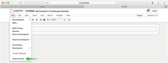
Figure 1-16. Close and halt a running notebook
Listing 1-14. Monitor Docker Memory Usage
$ docker statsCONTAINER CPU % MEM USAGE / LIMIT MEM % NET I/O BLOCK I/O PIDScfef9714b1c5 0.00% 55.31MiB / 990.7MiB 5.58% 109kB / 12.4MB / 4 1.56MB 397kB
The Python machine learning library scikit-learn 11 has a module dedicated to loading canonical datasets and generating synthetic datasets: sklearn.datasets. Relaunch your notebook and load the make_classification function from this module (Listing 1-15, Figure 1-17), using the standard Python syntax for importing a function from a module. Examine memory usage once more (Listing 1-16).
Figure 1-17. Import make_classification
Listing 1-15. Import make_classification
In [1]: from sklearn.datasets import make_classificationListing 1-16. Monitor Docker Memory Usage
$ docker statsCONTAINER CPU % MEM USAGE / LIMIT MEM % NET I/O BLOCK I/O PIDScfef9714b1c5 0.04% 148.3MiB / 990.7MiB 14.97% 242kB / 49.3MB / 13 4.03MB 340kB
Next (Listing 1-17, Figure 1-18), you create a new classification dataset using the default values . You then use the %whos IPython magic command12 to display the size of the dataset in memory. After this, you examine memory usage (Listing 1-18).

Figure 1-18. Import make_classification
Listing 1-17. Create a New Classification Dataset Using Default Values
In [2]: X, y = make_classification()In [3]: %whosVariable Type Data/Info-------------------------------------------X ndarray 100x20: 2000 elems, type 'float64', 16000 bytesmake_classification function <function make_classification at 0x7feb192669d8>y ndarray 100: 100 elems, type 'int64', 800 bytes
Listing 1-18. Monitor Docker Memory Usage
$ docker statsCONTAINER CPU % MEM USAGE / LIMIT MEM % NET I/O BLOCK I/O PIDScfef9714b1c5 0.01% 152MiB / 990.7MiB 15.35% 268kB / 54.1MB / 13 4.1MB 926kB
So far you are minimally taxing your system. Take note of the size of the dataset, size in Python memory, and Docker system usage associated with this default classification dataset and then restart the Python kernel (Figure 1-19).
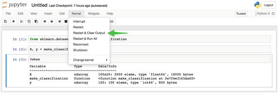
Figure 1-19. Restart the Python kernel
Next, you rerun the same experiment, increasing the size of your feature set by a factor of 10 (Listing 1-19, Figure 1-20). In Listing 1-20, you examine Docker system usage.

Figure 1-20. Import make_classification
Listing 1-19. Create a New Classification Dataset
In [2]: X, y = make_classification(n_samples=1000, n_features=20)In [3]: %whosVariable Type Data/Info-------------------------------------------X ndarray 100x20: 2000 elems, type `float64`, 160000 bytesmake_classification function <function make_classification at 0x7feb192669d8>y ndarray 100: 100 elems, type `int64`, 8000 bytes
Listing 1-20. Monitor Docker Memory Usage
$ docker statsCONTAINER CPU % MEM USAGE / LIMIT MEM % NET I/O BLOCK I/O PIDScfef9714b1c5 0.01% 149.7MiB / 990.7MiB 15.11% 286kB / 54.5MB / 13 4.13MB 1.13MB
Repeat the experiment several more times, capturing the results in Table 1-2. Each time, restart the kernel, create a new dataset that is 10 times larger than the previous, and then examine the result in terms of memory usage using the IPython magic command %whos and the docker stats tool.
Table 1-2. Classification Dataset Memory Footprint on t2.micro
Shape of Feature Set | Size in Python Memory | Docker System Usage |
|---|---|---|
100 × 20 | .016MB | 152MB |
1000 × 20 | .16MB | 149.7MB |
1000 × 200 | 1.525MB | 152.8MB |
10000 × 200 | 15.25MB | 162.6MB |
10000 × 2000 | 152.6MB | 279.7MB |
100000 × 2000 | Memory Exception | N/A |
Restart the Python kernel after each dataset is created. Take note of the dataset size that causes a memory exception.
When you attempt to create a classification dataset of size 100000 by 2000, you will hit a MemoryError, as seen in Listing 1-21 and Figure 1-21.

Figure 1-21. MemoryError when attempting to create a classification dataset
Listing 1-21. MemoryError When Attempting to Create a Classification Dataset
In [2]: X, y = make_classification(n_samples=100000, n_features=2000)---------------------------------------------------------------------------MemoryError Traceback (most recent call last)<ipython-input-2-df42c0ced9d5> in <module>()----> 1 X, y = make_classification(n_samples=100000, n_features=2000)/opt/conda/lib/python3.5/site-packages/sklearn/datasets/samples_generator.py in make_classification(n_samples, n_features, n_informative, n_redundant, n_repeated, n_classes, n_clusters_per_class, weights, flip_y, class_sep, hypercube, shift, scale, shuffle, random_state)179180 # Initialize X and y--> 181 X = np.zeros((n_samples, n_features))182 y = np.zeros(n_samples, dtype=np.int)183MemoryError:
And with that, you have hit the memory ceiling for your current system. It is not a particularly large dataset: 100,000 rows and 2000 columns. But then again, you are not working with a particularly large system either: a single CPU and 1GB of RAM. Certainly, you can imagine situations in which you will want to work with larger datasets on larger systems.
What Size Dataset Is Too Large to Be Used to Fit Different Kinds of Simple Models ?
Next, let’s answer the second question. Let’s do this by starting with a fresh Docker container. First, in Listing 1-22, you again use docker ps to display running containers.
Listing 1-22. Monitor Running Docker Containers
$ docker psCNID IMAGE COMMAND CREATED STATUS PORTS NAMEScfef jupyter/ "tini..." 53 min ago Up 53 min 0.0.0.0:8888-> friendly_ scipy... 8888/tcp curie
In Listing 1-23, you stop and then remove this container.
Listing 1-23. Stop and Remove a Running Container
$ docker stop friendly_curiefriendly_curieubuntu@ip-172-31-1-64:∼$ docker rm friendly_curiefriendly_curie
Next, in Listing 1-24, you launch a brand new jupyter/scipy-notebook container.
Listing 1-24. Run Jupyter Notebook Server
$ docker run -p 8888:8888 jupyter/scipy-notebook[I 20:05:42.246 NotebookApp] Writing notebook server cookie secret to /home/jovyan/.local/share/jupyter/runtime/notebook_cookie_secret...Copy/paste this URL into your browser when you connect for the first time,to login with a token:http://localhost:8888/?token=7a65c3c7dc6ea294a38397a48cc1ffe110ea138aef6d42c4
Make sure to take note of the new security token (7a65c3c7dc6ea294a38397a48cc1ffe110ea138aef6d42c4) and again use the AWS instance’s IP address in lieu of localhost (Listing 1-25).
Listing 1-25. The URL of the New Jupyter Instance Running on AWS with an Access Token Passed as a Query Parameter
http://54.244.109.176:8888/?token=7a65c3c7dc6ea294a38397a48cc1ffe110ea138aef6d42c4Before you start, measure the baseline usage for this current container via docker stats (Listing 1-26).
Listing 1-26. Monitor Docker Memory Usage
$ docker statsCONTAINER CPU % MEM USAGE / LIMIT MEM % NET I/O BLOCK I/O PIDS22efba43b763 0.00% 43.29MiB / 990.7MiB 4.37% 768B / 0B / 0B 2 486B
You again create a new Python 3 Notebook and set out to answer this second question. In Listing 1-27, you examine the memory usage of your Docker machine with a brand new notebook running.
Listing 1-27. Monitor Docker Memory Usage
$ docker statsCONTAINER CPU % MEM USAGE / LIMIT MEM % NET I/O BLOCK I/O PIDS22efba43b763 0.04% 90.69MiB / 990.7MiB 9.15% 58.8kB / 0B / 217kB 13 1.3MB
The approach to solving this problem will be slightly different and will make heavier use of docker stats. The %whos IPython magic command cannot be used to display memory usage of a fit model and, in fact, a trivial method for measuring memory usage does not exist.13 You will take advantage of your knowledge of the space in memory occupied by the data created by make_classification and this baseline performance you just measured.
You will use the code pattern in Listing 1-28 to perform this analysis.
Listing 1-28. Create a New Classification Dataset and Perform Naïve Model Fit
from sklearn.datasets import make_classificationfrom sklearn.<model_module> import <model>X, y = make_classification(<shape>)model = <model>()model.fit(X, y)model.score(X, y)
For example, use the following code to fit the smallest KNeighborsClassifier (Listing 1-29), DecisionTreeClassifier (Listing 1-30), LogisticRegression (1-31), and SVC (Listing 1-32). You will then modify the scope of the data for each subsequent test.
Listing 1-29. Fit the smallest KNeighborsClassifier
from sklearn.datasets import make_classificationfrom sklearn.neighbors import KNeighborsClassifierX, y = make_classification(1000, 20)model = KNeighborsClassifier()model.fit(X, y)model.score(X, y)
Listing 1-30. Fit the smallest DecisionTreeClassifier
from sklearn.datasets import make_classificationfrom sklearn.tree import DecisionTreeClassifierX, y = make_classification(1000, 20)model = DecisionTreeClassifier()model.fit(X, y)model.score(X, y)
Listing 1-31. Fit the smallest LogisticRegression
from sklearn.datasets import make_classificationfrom sklearn.linear_model import LogisticRegressionX, y = make_classification(1000, 20)model = LogisticRegression()model.fit(X, y)model.score(X, y)
Listing 1-32. Fit the smallest SVC
from sklearn.datasets import make_classificationfrom sklearn.neighbors import SVCX, y = make_classification(1000, 20)model = SVC()model.fit(X, y)model.score(X, y)
You then use docker stats to examine the Docker system usage. In between each test, you use docker restart (Listing 1-33) followed by the container id 22efba43b763 to reset the memory usage on the container. After restart the container, you will typically have to confirm restarting the Jupyter kernel as well (Figure 1-22).
Figure 1-22. Confirm a restart of the Jupyter kernel
Listing 1-33. Restart Your Docker Container
$ docker restart 22efba43b763The results of this experiment are captured in Table 1-3 and Figure 1-23.
Table 1-3. Classification of Dataset and Model Memory Footprint on t2.micro
Shape of Feature Set | Model Type | Dataset System Usage (MB) | Dataset and Fit Peak System Usage (MB) | Difference (MB) |
|---|---|---|---|---|
Baseline (No Notebook running) | N/A | N/A | N/A | 40.98 |
Baseline (Notebook running) | N/A | N/A | N/A | 76.14 |
100 × 20 | KNeighborsClassifier | 99.9 | 100.0 | 0.1 |
100 × 20 | DecisionTreeClassifier | 103.2 | 103.3 | 0.1 |
100 × 20 | LogisticRegression | 102.5 | 102.6 | 0.1 |
100 × 20 | SVC | 101.2 | 101.4 | 0.2 |
1000 × 20 | KNeighborsClassifier | 100.3 | 100.4 | 0.1 |
1000 × 20 | DecisionTreeClassifier | 103.7 | 103.8 | 0.1 |
1000 × 20 | LogisticRegression | 104.9 | 105.1 | 0.2 |
1000 × 20 | SVC | 104.9 | 105.5 | 0.6 |
1000 × 200 | KNeighborsClassifier | 106.3 | 106.9 | 0.6 |
1000 × 200 | DecisionTreeClassifier | 104.8 | 105.7 | 0.9 |
1000 × 200 | LogisticRegression | 102.0 | 102.3 | 0.3 |
1000 × 200 | SVC | 104.6 | 106.0 | 1.4 |
10000 × 200 | KNeighborsClassifier | 115.5 | 117.8 | 2.3 |
10000 × 200 | DecisionTreeClassifier | 119.8 | 127.8 | 8.0 |
10000 × 200 | LogisticRegression | 121.3 | 122.6 | 1.3 |
10000 × 200 | SVC | 121.1 | 286.7 | 165.6 |
10000 × 2000 | KNeighborsClassifier | 256.4 | 275.1 | 18.7 |
10000 × 2000 | DecisionTreeClassifier | 257.1 | 333.6 | 76.5 |
10000 × 2000 | LogisticRegression | 258.6 | 564.9 | 306.3 |
10000 × 2000 | SVC | 256.3 | 491.9 | 235.6 |

Figure 1-23. Dataset vs. Peak Usage by model
Measuring Scope of Data Capable of Fitting on T2.Micro
In the previous test, a 10000 row x 2000 column dataset was the largest that you were able to successfully load into memory. In this test, you were able to successfully fit a naïve implementation of four different machine learning models against each of the datasets that you were able to load into memory. That said, you can see that neither the LogisticRegression nor the SVC (Support Vector Classifier) are capable of handling much more.
Summary
In this chapter, I introduced the core subjects of this text, Docker and Jupyter, and discussed a recommended practice for working through this text, which is using a disposable Linux instance on Amazon Web Services. I provided detailed instructions for configuring, launching, and provisioning such an instance. Having launched an instance, you used Docker and Jupyter to explore a toy big data example, diagnosing memory performance as you loaded and fit models using a synthetic classification dataset generated by scikit-learn.
I did not intended for this chapter to have been the moment when you thoroughly grasped using Docker and Jupyter to build systems for performing data science. Rather, I hope that it has served as a substantive introduction to the topic. Rather than simply stating what Docker and Jupyter are, I wanted you to see what these two technologies are by using them.
In the chapters ahead, you will explore many aspects of the Docker and Jupyter ecosystems. Later, you will learn about the open source data stores Redis, MongoDB, and PostgreSQL, and how to integrate them into your Docker-based applications. Finally, you will learn about the Docker Compose tool and how to tie all of these pieces together in a single docker-compose.yml file.
Footnotes
4 Instructions for creating a new AWS account can be found at https://aws.amazon.com/premiumsupport/knowledge-center/create-and-activate-aws-account/ .
10 My t2.micro has but a single CPU.