
Throughout this book we have seen many examples of CGI scripts generating dynamic output. However, in almost all cases, the output has been HTML. Certainly this is the most common format your scripts will generate. However, CGI scripts can actually generate any type of format, and in this chapter we will look at how we can dynamically generate images.
Generating images dynamically has many uses. One of the most common is to generate graphs. If you have a data source that is continually changing, such as the results of an online survey, a CGI script can generate a graph that presents a visual snapshot of this data.
There are also times when generating images dynamically makes less sense. It is much less efficient to generate an image dynamically than for your web server to serve the image from an image file. Thus, just because some of these tools allow you to generate really cool graphics dynamically doesn’t mean you must use them only in a dynamic context. Unless the images you generate are based upon data that changes, save the image to a static file and serve that instead.
This chapter presents a broad overview of the different tools available for generating dynamic images online, and includes references with each for finding more information. The goal of this chapter is to explain techniques for generating images dynamically and familiarize you with the most popular tools available to you. A full description of many of these tools along with others is available in a book of its own, Programming Web Graphics with Perl and GNU Software by Shawn Wallace (O’Reilly & Associates, Inc.).
Let’s first review the image formats that are used online today. The most common image formats, of course, are GIF and JPEG, which every graphical web browser supports. Other file formats that we will discuss in this chapter include PNG and PDF.
The Graphics Interchange Format (GIF ) was created by CompuServe and released as an open standard in 1987. It quickly became a very popular image format and, along with JPEG, became a standard format for images on the Web. GIF files are typically quite small, especially for images with few colors, which makes them well suited for transferring online.
GIF only supports up to 256 colors, but it works well for text and images, such as icons, which do not have many colors but have sharp details. The compression algorithm that GIF uses, LZW, is lossless, which means that no image quality is lost during compression or decompression, allowing GIF files to accurately capture details.
The GIF file format has been extended to support basic animation, which can loop. The moving banner ads that you see online are typically animated GIF files. GIF files can also have a transparent background by specifying a single color in the image that should be displayed as transparent.
Unfortunately, CompuServe and others apparently failed to notice that LZW, the compression algorithm used by GIF, was actually patented by Unisys in 1983. Unisys reportedly discovered that GIF uses LZW in the early 1990s and in 1994 CompuServe and Unisys reached a settlement and announced that developers who write software supporting GIF must pay a licensing fee to Unisys. Note that this does not include web authors who use GIF files or users who browse them on the Web.
This turn of events created quite a stir among developers, especially open source developers. As a result, CompuServe and others developed the PNG format as a LZW-free successor to GIF; we’ll discuss PNG below. However, GIF remains a very popular file format, and PNG is not supported by all browsers.
As a result of the LZW licensing issue, the tools we discuss in this chapter provide very limited support for GIF files, as we will see.
The Portable Network Graphic (PNG ) format was created as a successor to the GIF format. It adds the following features over GIF:
PNG uses an efficient compression algorithm that is not LZW. In most cases, it achieves slightly better compression than the LZW algorithm.
PNG supports images in any of three modes: images with a limited palette of 256 or fewer colors, 16-bit grayscale images, and 48-bit true color images.
PNG supports alpha channels, which allows varying degrees of transparency.
PNG graphics have a better interlacing algorithm that allows users to make out the contents of the image as it downloads much faster than with a GIF.
For additional differences, as well as an demonstration of the difference between the PNG and GIF interlacing, visit http://www.cdrom.com/pub/png/pngintro.html.
Unfortunately, many browsers do not support PNG images. Of those that do, many do not support all of its features, such as multiple levels of transparency. Support for PNG should continue to increase, however, and older browsers that do not support it will eventually be upgraded.
PNG does not support animations.
The Joint Photographic Experts Group (JPEG ) is a standards body created to generate an image format for encoding continuous tone images. Their JPEG standard actually discusses a very general method for still image compression and not a file format. The file format that people typically think of as a JPEG is actually JFIF, the JPEG File Interchange Format . We will stick with the more familiar term and also refer to a JFIF file as a JPEG file.
JPEG files are ideal for encoding photographs. JPEG supports full, 24-bit color but it uses a lossy compression algorithm, which means that each time the file is compressed, detail is lost. Because the encoding for JPEG files is done in blocks, it is most noticeable in images that have very sharp details, such as text and line art. These details may appear blurred in a JPEG file.
Adobe’s Portable Document Format (PDF ) is more than just an image format. It is actually a language derived from PostScript that can include text, basic shapes, line art, and images, as well as numerous other elements. Unlike images, which are typically displayed within an HTML file, PDF files are typically standalone documents, and users use a browser plug-in or external application such as Adobe Acrobat to view them.
There are a few specific issues we encounter when outputting image data that we do not normally encounter when we generate HTML. So before we look at how we can create our own images, let’s take a look at these issues.
Example 13.1 shows a CGI script that returns a random image each time it is called.
Example 13-1. random_image.cgi
#!/usr/bin/perl -wT

use strict;
use CGI;
use CGI::Carp;

use constant BUFFER_SIZE     => 4_096;
use constant IMAGE_DIRECTORY => "/usr/local/apache/data/random-images";

my $q = new CGI;
my $buffer = "";

my $image = random_file( IMAGE_DIRECTORY, '\.(png|jpg|gif)$' );
my( $type ) = $image =~ /.(w+)$/;
$type eq "jpg" and $type = "jpeg";

print $q->header( -type => "image/$type", -expires => "-1d" );
binmode STDOUT;

local *IMAGE;
open IMAGE, IMAGE_DIRECTORY . "/$image" or die "Cannot open file $image: $!";
while ( read( IMAGE, $buffer, BUFFER_SIZE ) ) {
    print $buffer;
}
close IMAGE;


# Takes a path to a directory and an optional filename mask regex
# Returns the name of a random file from the directory
sub random_file {
    my( $dir, $mask ) = @_;
    my $i = 0;
    my $file;
    local *DIR, $_;

    opendir DIR, $dir or die "Cannot open $dir: $!";
    while ( defined ( $_ = readdir DIR ) ) {
        /$mask/o or next if defined $mask;
        rand ++$i < 1 and $file = $_;
    }
    closedir DIR;
    return $file;
}
This CGI script starts like our other CGI scripts, but the
random_file function requires a little
explanation. We pass the random_file function
the path to our image directory and a regular expression that matches
GIF, PNG, and JPEG files extensions. The
algorithm that
random_file uses is adopted from an algorithm
for selecting a random line from a
text file that appears
in the perlfaq5 manpage (it originally
appeared in Programming Perl ):
rand($.) > 1 && ( $line = $_ ) while <>;
This code selects a line from a text file, by reading the file only
once, and needing to store only two lines in memory at a time. It
always sets $line to the first line, then there is
a one in two chance that it will set it to the second line, a one in
three chance for the third line, etc. The probabilities always
balance out, no matter how many lines are in the file.
Likewise, we apply this technique to reading files in a directory. We first discard any files that do not match our mask if we supplied a mask. We then apply the algorithm to determine whether to store the current filename. The last filename we happen to store is what we ultimately return.
Now we return to the body of our CGI script and use the extension of the file to determine the media type of our image. Because the media type for JPEG files (image/jpeg) differs from the common extension for JPEGs (.jpg), we convert these.
Next we print our header with the corresponding media type for our image as well as an Expires header to discourage the browser from caching this response. Unfortunately, this header does not always work; we will discuss this further in a moment.
After printing our header, we use Perl’s built-in function
binmode
to indicate that we are
outputting binary data. This is important. On
Unix systems,
binmode does nothing (thus on these systems it can be
omitted), but on Windows, MacOS, and other operating systems that do
not use a single newline as an end-of-line character, it disables
automatic end-of-line translation that may otherwise corrupt binary
output.
Finally, we read and output the image data. Note that
because it is a binary file, there are no standard line endings, so
we must use read instead of
<> used
on text files.
You can include a dynamic image in one of your HTML documents the same way you include standard images: via a URL. For example, the following tag displays a random image using our previous example:
<IMG SRC="/cgi/random_image.cgi" >
Unfortunately, there are some browsers (specifically some versions of Internet Explorer) that sometimes pay more attention to the extension of a resource they are fetching than to the HTTP media type header. According to the HTTP standard, this is wrong of course, and probably an accidental bug, but if you want to accommodate users of these browsers, you may wish to append redundant path information onto URLs to provide an acceptable file extension:
<IMG SRC="/cgi/survey_graph.cgi/survey.png" >
The web server will still execute survey_graph.cgi, which generates the image while ignoring the additional /survey.png path information.
Incidentally, adding false path information like this is a good idea whenever your CGI script is generating content that you expect users to save, because browsers generally default to the filename of the resource they requested, and the user probably would rather the file be saved as survey.png than survey_graph.cgi.
For CGI scripts like random_image.cgi that
determine the filename and/or extension dynamically, you can still
accomplish this with redirection. For example, we could replace the
line that sets $image in
random_image.cgi (Example 13.1)
with the following lines:
my( $image ) = $q->path_info =~ /(w+.w+)$/;

unless ( defined $image and -e IMAGE_DIRECTORY . "/$image" ) {
    $image = random_file( IMAGE_DIRECTORY, '\.(png|jpg|gif)$' );
    print $q->redirect( $q->script_name . "/$image" );
    exit;
}
The first time this script is accessed, there is no additional path
information, so it fetches a new image from our
random_file function and redirects to itself
with the filename appended as path information. When this second
request arrives, the script retrieves the filename from the path
information and uses this if the filename matches our regular
expression and it exists. If it isn’t a valid filename, the
script acts as if no path had been passed and generates a new
filename.
Note that our filename regular expression,
/(w+.w+)$/, prevents any images in our image
directory that have characters not matched by w
from being displayed, including images that contain hyphens.
Depending on the filenames you are using, you may need to adjust this
pattern.
In Example 13.1, we generated an Expires HTTP header in order to discourage caching. Unfortunately, not all browsers respect this header, so it is quite possible for a user to get a stale image instead of a dynamic one. Some browsers also try to determine whether a resource is generated dynamically by something such as a CGI script or whether it is static; these browsers seem to assume that images are static, especially if you append additional path information as we just discussed.
There is a way to force browsers not to cache images, but this requires that the tag for the image also be dynamically generated. In these circumstances, you can add a value that constantly changes, such as the time in seconds, to the URL:
my $time = time;
print $q->img( { -src => "/cgi/survey_graph.cgi/$time/survey.png" } );
By adding the time to the additional path information, the browser views each request (more than a second apart) as a new resource. However, this technique does fill the browser’s cache with duplicate images, so use it sparingly, and always combine this with an Expires header for the sake of browsers that support it. Adding a value like this to the query string also works:
print $q->img( { -src => "/cgi/survey_graph.cgi/survey.png?random=$time" } );If nothing else on the HTML page is dynamic, and you do not wish to convert it to a CGI script, then you can also accomplish this via a server-side include (see Chapter 6):
<!--#config timefmt="%d%m%y%H%M%S" -->
<IMG SRC="/cgi/survey_graph.cgi/<!--#echo var="DATE_LOCAL"-->/survey.png">
Although this is a little hard to read and is syntactically invalid HTML, the SSI tag will be parsed by an SSI-enabled server and replaced with a number representing the current date and time before it is sent to the user.
The GD module was created and is maintained by Lincoln Stein, who is also the author of CGI.pm. GD provides a Perl port of the gd graphics library created by Thomas Boutell for the C programming language. The gd library was originally created for creating and editing GIFs. As a result of the Unisys patent issue, however, it was rewritten for PNG (incidentally, Thomas Boutell was a co-author and the editor for the PNG specification). Current versions of the gd library and the GD module no longer support GIFs, and older versions are no longer distributed. If you have an older version of these modules (for example, an older version was included with your system) that does support GIFs, you should probably contact Unisys for licensing terms and/or an attorney familiar with patent issues before using them.
You can install GD just like other CPAN modules, except that you should ensure that you have the latest version of gd. GD contains C code that must be compiled with gd, and if you have an older version of gd, or if gd is missing, you will get errors during compilation.
The gd library is available at http://www.boutell.com/. This site also has instructions for building gd plus references to other optional packages that gd uses if available, such as the FreeType engine, which enables gd (and thus GD) to support TrueType fonts. Note that gd requires the latest versions of libpng and zlib; you can find links to these libraries at http://www.boutell.com/ too.
In this section, we’ll develop an application that uses the uptime Unix system command to plot the system load average (see Figure 13.1). As we will see in the next section, there are modules to help us generate graphs more easily, but let’s first see gd ’s graphics primitives in action.
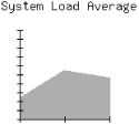
The application itself is rather straightforward. First, we invoke the uptime command, which returns three values, representing the load averages for the previous 5, 10 and 15 minutes, respectively—though this may differ among the various Unix implementations. Here is the output of an uptime command:
2:26pm up 11:07, 12 users, load average: 4.63, 5.29, 2.56
Then, we use gd’s various drawing primitives, such as lines and polygons to draw the axes and scale and to plot the load values.
Example 13.2 shows the code.
Example 13-2. loads.cgi
#!/usr/bin/perl -wT

use strict;

use CGI;
use GD;

BEGIN {
    $ENV{PATH} = '/bin:/usr/bin:/usr/ucb:/usr/local/bin';
    delete @ENV{ qw( IFS CDPATH ENV BASH_ENV ) };
}

use constant LOAD_MAX       => 10;

use constant IMAGE_SIZE     => 170;     # height and width
use constant GRAPH_SIZE     => 100;     # height and width
use constant TICK_LENGTH    => 3;

use constant ORIGIN_X_COORD => 30;
use constant ORIGIN_Y_COORD => 150;

use constant TITLE_TEXT     => "System Load Average";
use constant TITLE_X_COORD  => 10;
use constant TITLE_Y_COORD  => 15;

use constant AREA_COLOR     => ( 255, 0, 0 );
use constant AXIS_COLOR     => ( 0, 0, 0 );
use constant TEXT_COLOR     => ( 0, 0, 0 );
use constant BG_COLOR       => ( 255, 255, 255 );

my $q     = new CGI;
my @loads = get_loads(  );

print $q->header( -type => "image/png", -expires => "-1d" );

binmode STDOUT;
print area_graph( @loads );


# Returns a list of the average loads from the system's uptime command
sub get_loads {
    my $uptime = `uptime` or die "Error running uptime: $!";
    my( $up_string ) = $uptime =~ /average: (.+)$/;
    my @loads = reverse
                map { $_ > LOAD_MAX ? LOAD_MAX : $_ }
                split /,s*/, $up_string;
    @loads or die "Cannot parse response from uptime: $up_string";
    return @loads;
}


# Takes a one-dimensional list of data and returns an area graph as PNG
sub area_graph {
    my $data = shift;

    my $image = new GD::Image( IMAGE_SIZE, IMAGE_SIZE );
    my $background = $image->colorAllocate( BG_COLOR );
    my $area_color = $image->colorAllocate( AREA_COLOR );
    my $axis_color = $image->colorAllocate( AXIS_COLOR );
    my $text_color = $image->colorAllocate( TEXT_COLOR );

    # Add Title
    $image->string( gdLargeFont, TITLE_X_COORD, TITLE_Y_COORD,
                    TITLE_TEXT, $text_color );

    # Create polygon for data
    my $polygon = new GD::Polygon;
    $polygon->addPt( ORIGIN_X_COORD, ORIGIN_Y_COORD );

    for ( my $i = 0; $i < @$data; $i++ ) {
        $polygon->addPt( ORIGIN_X_COORD + GRAPH_SIZE / ( @$data - 1 ) * $i,
                         ORIGIN_Y_COORD - $$data[$i] * GRAPH_SIZE / LOAD_MAX );
    }

    $polygon->addPt( ORIGIN_X_COORD + GRAPH_SIZE, ORIGIN_Y_COORD );

    # Add Polygon
    $image->filledPolygon( $polygon, $area_color );

    # Add X Axis
    $image->line( ORIGIN_X_COORD, ORIGIN_Y_COORD,
                  ORIGIN_X_COORD + GRAPH_SIZE, ORIGIN_Y_COORD,
                  $axis_color );
    # Add Y Axis
    $image->line( ORIGIN_X_COORD, ORIGIN_Y_COORD,
                  ORIGIN_X_COORD, ORIGIN_Y_COORD - GRAPH_SIZE,
                  $axis_color );

    # Add X Axis Ticks Marks
    for ( my $x = 0; $x <= GRAPH_SIZE; $x += GRAPH_SIZE / ( @$data - 1 ) ) {
        $image->line( $x + ORIGIN_X_COORD, ORIGIN_Y_COORD - TICK_LENGTH,
                      $x + ORIGIN_X_COORD, ORIGIN_Y_COORD + TICK_LENGTH,
                      $axis_color );
    }

    # Add Y Axis Tick Marks
    for ( my $y = 0; $y <= GRAPH_SIZE; $y += GRAPH_SIZE / LOAD_MAX ) {
        $image->line( ORIGIN_X_COORD - TICK_LENGTH, ORIGIN_Y_COORD - $y,
                      ORIGIN_X_COORD + TICK_LENGTH, ORIGIN_Y_COORD - $y,
                      $axis_color );
    }

    $image->transparent( $background );

    return $image->png;
}
After importing our modules, we use a
BEGIN
block to make the environment
safe for taint. We have to do this because our script will use the
external uptime command (see Section 8.4).
Then we set a large number of constants. The
LOAD_MAX constant sets the upper limit on the
load average. If a load average exceeds the value of 10, then it is
set to 10, so we don’t have to worry about possibly scaling the
axes. Remember, the whole point of this application is not to create
a highly useful graphing application, but one that will illustrate
some of GD’s drawing primitives.
Next, we choose a size for our graph area,
GRAPH_SIZE, as well as for the image itself,
IMAGE_SIZE. Both the image and the graph are
square, so these sizes represent length as well as width.
TICK_LENGTH corresponds to the length of each tick
mark (this is actually half the length of the tick mark once
it’s drawn).
ORIGIN_X_COORD and
ORIGIN_Y_COORD contain the coordinates of the
origin of our graph (its lower left-hand corner).
TITLE_TEXT, TITLE_X_COORD, and
TITLE_Y_COORD contain values for the title of our
graph. Finally, we set AREA_COLOR,
AXIS_COLOR, TEXT_COLOR, and
BG_COLOR to an array of three numbers containing
red, green, and blue values, respectively; these values range from
0 to 255.
The system’s load is returned by
get_loads. It takes the output of
uptime
, parses out the load averages,
truncates any average greater than the value specified by
UPPER_LIMIT, and reverses the values so they are
returned from oldest to newest. Thus, our graph will plot from left
to right the load average of the system over the last 15, 10, and 5
minutes.
Returning to the main body of our CGI script, we output our header,
enable binary mode, then fetch the data for our PNG from
area_graph and print it.
The area_graph
function contains all of our image
code. It accepts a reference to an array of data points, which it
assigns to $data. We first create a new instance
of GD::Image, passing to it the dimensions
of the canvas that we want to work with.
Next, we allocate four colors that correspond to our earlier constants. Note that the first color we allocate automatically becomes the background color. In this case, the image will have a white background.
We use the string method to display our title
using the gdLarge font. Then, we draw two lines,
one horizontal and one vertical from the origin, representing the x
and y axes. Once we draw the axes, we iterate through the entire
graph area and draw the tick marks on the axes.
Now, we’re ready to plot the load averages on the graph. We create a new instance of the GD::Polygon class to draw a polygon with the vertices representing the three load averages. Drawing a polygon is similar in principle to creating a closed path with several points.
We use the addPt method to add a point to the
polygon. The origin is added as the first point. Then, each load
average coordinate is calculated and added to the polygon. We add a
final point on the x axis. GD automatically connects the final point
to the first point.
The filledPolygon method fills the polygon
specified by the $polygon object with the
associated color. And finally, the graph is rendered as a PNG and the
data is returned.
GD supports many methods beyond those listed here, but we do not have space to list them all here. Refer to the GD documentation or Programming Web Graphics for full usage.
Several modules are available on CPAN that work with GD. Some provide convenience methods that make it easier to interact with GD. Others use GD to create graphs easily. In this section, we will look at GD::Text, which helps place text in GD images, and GD::Graph, the most popular graphing module, along with extensions provided by GD::Graph3D.
GD::Text is collection of modules for managing text, written by Martin Verbruggen. GD::Text provides three modules for working with text in GD images: GD::Text provides information about the size of text in GD, GD::Text::Align allows us to place text in GD with greater control, and GD::Text::Wrap allows us to place text boxes containing wrapped text. We don’t have the space to cover all three of these modules in detail, but let’s take a look at what is probably the most useful of these modules, GD::Text::Align.
In our previous example, loads.cgi, we used preset constants to determine the starting position of our centered title, “System Load Average.” These values are derived from trial and error, and although not elegant, this approach works for images when the title is fixed. However, if someone decides to change the title of this image, the coordinates also need to be adjusted to keep the new title centered horizontally. And for images with dynamic titles, this approach will simply not work. A much better solution would be to calculate the title’s placement dynamically.
GD::Text::Align allows us to do this easily. In the above example,
the TITLE_Y_COORD constant is really the top
margin, and TITLE_X_COORD is the left margin
(remember coordinates start at the top left corner of the image in
GD). There is nothing wrong with a constant for the top margin, but
if we want to have a centered title, then we should calculate
TITLE_X_COORD dynamically.
Thus, let’s look at how we could modify loads.cgi to do this with GD::Text::Align. First, let’s include the GD::Text::Align module at the start of the script:
use GD::Text::Align;
Next, we can replace the line that places the title string (in the
area_graph subroutine) with the following:
# Add Centered Title
my $title = GD::Text::Align->new(
    $image,
    font    => gdLargeFont,
    text    => TITLE_TEXT,
    color   => $text_color,
    valign  => "top",
    halign  => "center",
);
$title->draw( IMAGE_SIZE / 2, TITLE_Y_COORD );
We create a GD::Text::Align object by passing our GD object,
$image, and a number of parameters describing our
text, and the draw method adds our title to the
image. We should then remove the TITLE_X_COORD
constant, which we know longer use; you may also want to rename
TITLE_Y_COORD to something more meaningful in this
context, such as TITLE_TOP_MARGIN.
Besides allowing you to place aligned text, GD::Text::Align also lets you obtain coordinates for the bounding box for a text string before you place it so you can make adjustments if necessary (such as reducing the size of the font). It also supports True Type fonts and placing text at angles. Refer to the GD::Text::Align online documentation for more information.
GD::Graph, also by Martin Verbruggen, is
a collection of modules that produce graphs using GD. GD::Graph has
had a few different names within the last year. It was originally
called GIFgraph.
However, after GD removed support for GIF, it no longer produced
GIFs; in fact, it broke. Steve Bonds updated it to use PNG and
renamed it as
Chart::PNGgraph.
Later, Martin Verbruggen gave it the more general name, GD::Graph,
and removed specific image format support. Previously, you called the
plot method to retrieve the graph in either GIF
(for GIFgraph) or PNG (for PNGgraph) formats. Now,
plot returns a GD::Image object so the
user can choose the format desired. We’ll see how this works in
a moment.
To install GD::Graph, you must first have GD and GD::Text installed. GD::Graph provides the following modules for creating graphs:
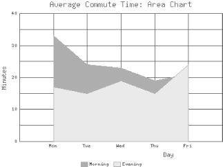
GD::Graph::area creates area charts, as shown in Figure 13.2.
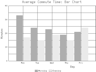
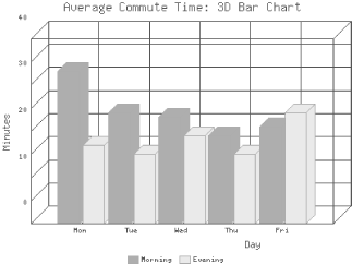
GD::Graph::bars creates bar charts, as shown in Figure 13.3.
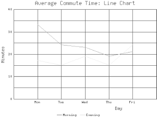
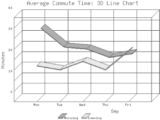
GD::Graph::lines creates line charts, as shown in Figure 13.4.
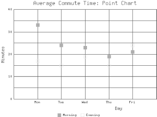
GD::Graph::points creates point charts (also sometimes called XY or scatter charts), as shown in Figure 13.5.
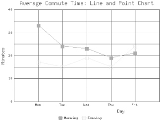
GD::Graph::linespoints creates a combination of line and point charts, as shown in Figure 13.6.
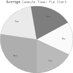
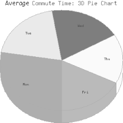
GD::Graph::pie creates pie charts, as shown in Figure 13.7.
GD::Graph::mixed allows you to create a combination of any of the previous types except pie charts, as shown in Figure 13.8.
Each of the previous examples uses the data shown in Table 13.1.
Table 13-1. Sample Daily Commute Time in Minutes
|
Weekday |
Monday |
Tuesday |
Wednesday |
Thursday |
Friday |
|---|---|---|---|---|---|
|
Morning |
33 |
24 |
23 |
19 |
21 |
|
Evening |
17 |
15 |
19 |
15 |
24 |
Example 13.3 contains the code used to create the mixed graph that appears in Figure 13.8.
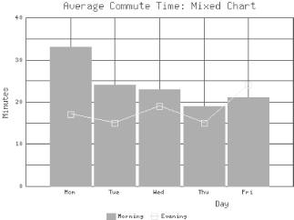
Example 13-3. commute_mixed.cgi
#!/usr/bin/perl -wT

use strict;
use CGI;
use GD::Graph::mixed;

use constant TITLE => "Average Commute Time: Mixed Chart";

my $q     = new CGI;
my $graph = new GD::Graph::mixed( 400, 300 );
my @data  = (
    [ qw( Mon  Tue  Wed  Thu  Fri ) ],
    [      33,  24,  23,  19,  21   ],
    [      17,  15,  19,  15,  24   ],
);


$graph->set(
    title           => TITLE,
    x_label         => "Day",
    y_label         => "Minutes",
    long_ticks      => 1,
    y_max_value     => 40,
    y_min_value     => 0,
    y_tick_number   => 8,
    y_label_skip    => 2,
    bar_spacing     => 4,
    types           => [ "bars", "linespoints" ],
);

$graph->set_legend( "Morning", "Evening" );
my $gd_image = $graph->plot( @data );

print $q->header( -type => "image/png", -expires => "now" );

binmode STDOUT;
print $gd_image->png;
Note that for this script we do not need to use the GD module because we are not creating images directly; we simply use the GD::Graph module. We set one constant for the title of the graph. We could have created many more constants for the different parameters we are passing to GD::Graph, but this script is short, and not using constants allows you to easily see the values each parameter takes.
We create a mixed graph object by passing the width and height in
pixels, and we set up our data. Then, we call the
set method to set parameters for our graph. The
meaning of some of these parameters is obvious; we will just explain
those that may not be. long_ticks sets whether
ticks should extend through the area of the chart to form a grid.
y_tick_number specifies how many ticks the y axis
should be divided into. y_label_skip sets how
often the ticks on the y axis should be labelled; our setting,
2, means every other one.
bar_spacing is the number of pixels between the
bars (for the bars series). Finally, types sets
the graph type of each series.
We add a legend that describes our data series. Next, we call the plot method with our data and receive a GD::Image object containing our new graph. Then all we need to do is generate our header and output the image as a PNG.
We won’t look at code for each image type, because except for
pie charts, this same code can generate each of the other types of
images with very few modifications. You simply need to change
GD::Graph::mixed to the name of the module you wish to use. The only
property in the set method here that is particular to mixed graphs is
types. The only property particular to mixed
charts or bar charts is bar_spacing. The others
are common across all the
other types.
Pie charts are somewhat different. They only accept a single data series, they cannot have a legend, and because they have no axes, most of the parameters we just discussed do not apply to them. Furthermore, pie charts are three-dimensional by default. Example 13.4 provides the code used to create the pie chart that’s shown in Figure 13.7.
Example 13-4. commute_pie.cgi
#!/usr/bin/perl -wT

use strict;
use CGI;
use GD::Graph::pie;

use constant TITLE => "Average Commute Time: Pie Chart";

my $q     = new CGI;
my $graph = new GD::Graph::pie( 300, 300 );
my @data  = (
    [ qw( Mon  Tue  Wed  Thu  Fri ) ],
    [      33,  24,  23,  19,  21   ]
);


$graph->set(
    title           => TITLE,
    '3d'            => 0
);

my $gd_image = $graph->plot( @data );

print $q->header( -type => "image/png", -expires => "-1d" );

binmode STDOUT;
print $gd_image->png;
This script is much shorter because we do not set nearly so many
parameters. Instead, we simply set the title and turn the
3d option off (we will return to this concept in
the next section). We also used 300 × 300 for the size of the
graph instead of 400 × 300. GD::Graph will scale a pie chart to
fit the edges of the graph, so pie charts will be elliptical if they
are plotted in a rectangular region. Finally, we submit only one
series of data and omit the call to add a legend, which is currently
unsupported for pie charts.
GD::Graph3D allows us to generate three-dimensional charts. It is an extension to GD::Graph that provides three additional modules:
GD::Graph::bars3d creates three-dimensional bar charts, as shown in Figure 13.9.
GD::Graph::lines3d creates three-dimensional line charts, as shown in Figure 13.10.
GD::Graph::pie3d creates three-dimensional pie charts, as shown in Figure 13.11. This module actually just calls GD::Graph::pie, which now generates three-dimensional pie charts by default anyhow. It is included simply to provide a name consistent with the other two modules. In order to make the usage clear and consistent, perhaps GD::Graph::pie will ultimately default to non-three-dimensional pie charts and GD::Graph::pie3d can become the preferred way to generate a 3D version.
In order to use these modules, simply replace the standard module name with the 3D module name; all other properties and methods remain the same. Additionally, the 3D bar chart and 3D line chart each offer methods to set the depth of the bars and lines. Refer to the included documentation. Note that although the module is distributed as GD::Graph3d, the documentation is installed, along with the additional graph types, in the GD/Graph directory, so to view the documentation for GD::Graph3d, you must reference it this way:
$ perldoc GD::Graph::Graph3d
PerlMagick is another graphics module designed to be used online. It is based upon the ImageMagick library, which is available for many languages on many different platforms. The Perl module, Image::Magick, is often referred to as PerlMagick. ImageMagick was written by John Cristy; the Perl module was written by Kyle Shorter.
ImageMagick is very powerful and supports the following operations:
- Identify
ImageMagick supports more than fifty different image file formats, including GIF, JPEG, PNG, TIFF, BMP, EPS, PDF, MPEG, PICT, PPM, and RGB.
- Convert
ImageMagick allows you to convert between these formats.
- Montage
ImageMagick can create thumbnails of images.
- Mogrify
ImageMagick can perform all sorts of manipulations on images including blur, rotate, emboss, and normalize, just to name a few.
- Drawing
Like GD, you can add basic shapes and text to images in ImageMagick.
- Composite
ImageMagick can merge multiple images.
- Animate
ImageMagick supports file formats with multiple frames, such as animated GIFs.
- Display
ImageMagick also includes tools, such as display, for displaying and manipulating images interactively.
We won’t cover all of these, of course. We’ll look at how to convert between different formats as well as how to create an image using some of the advanced effects.
You can obtain the Image::Magick module from CPAN, but it requires that the ImageMagick library be installed already. You can get ImageMagick from the ImageMagick home page, http://www.wizards.dupont.com/cristy/. This page contains links to many resources, including pre-compiled binary distributions of ImageMagick for many operating systems, detailed build instructions if you choose to compile it yourself, and a detailed PDF manual.
Image::Magick is much more powerful than GD. It supports numerous file formats and allows many types of operations, while GD is optimized for a certain set of tasks and a single file format. However, this power comes at a price. Whereas the GD module has relatively low overhead and is quite efficient, the Image::Magick module may crash unless it has at least 80MB of memory, and for best performance at least 64MB should be real RAM (i.e., not virtual memory).
Image::Magick supports GIFs. However, support for LZW compression is not compiled into ImageMagick by default. This causes GIFs that are created by Image::Magick to be quite large. It is possible to enable LZW compression when building ImageMagick, but of course you should check with Unisys about licensing and/or contact an attorney before doing so. Refer to the ImageMagick build instructions for more information.
As we noted earlier, unfortunately not all browsers support PNGs. Let’s see how we can use Image::Magick to convert a PNG to a GIF or a JPEG. In order to use an image in Image::Magick, you must read it from a file. According to the documentation, it should also accept input from a file handle, but as of the time this book was written, this feature is broken (it silently fails). We will thus write the output of GD to a temporary file and then read it back in to Image::Magick. Example 13.5 includes our earlier example, commute_pie.cgi , updated to output a JPEG instead unless the browser specifically states that it supports PNG files.
Example 13-5. commute_pie2.cgi
#!/usr/bin/perl -wT

use strict;
use CGI;
use GD::Graph::pie;
use Image::Magick;
use POSIX qw( tmpnam );
use Fcntl;

use constant TITLE => "Average Commute Time: Pie Chart";

my $q     = new CGI;
my $graph = new GD::Graph::pie( 300, 300 );
my @data  = (
    [ qw( Mon  Tue  Wed  Thu  Fri ) ],
    [      33,  24,  23,  19,  21   ],
);


$graph->set(
    title           => TITLE,
    '3d'            => 0
);

my $gd_image = $graph->plot( @data );
undef $graph;

if ( grep $_ eq "image/png", $q->Accept )
    print $q->header( -type => "image/png", -expires => "now" );
    binmode STDOUT;
    print $gd_image->png;
}
else {
    print $q->header( -type => "image/jpeg", -expires => "now" );
    binmode STDOUT;
    print_png2jpeg( $gd_image->png );
}

# Takes PNG data, converts it to JPEG, and prints it
sub print_png2jpeg {
    my $png_data = shift;
    my( $tmp_name, $status );

    # Create temp file and write PNG to it
    do {
        $tmp_name = tmpnam(  );
    } until sysopen TMPFILE, $tmp_name, O_RDWR | O_CREAT | O_EXCL;
    END { unlink $tmp_name or die "Cannot remove $tmp_name: $!"; }

    binmode TMPFILE;
    print TMPFILE $png_data;
    close TMPFILE;
    undef $png_data;

    # Read file into Image::Magick
    my $magick = new Image::Magick( format => "png" );
    $status = $magick->Read( filename => $tmp_name );
    warn "Error reading PNG input: $status" if $status;

    # Write file as JPEG to STDOUT
    $status = $magick->Write( "jpeg:-" );
    warn "Error writing JPEG output: $status" if $status;
}
We use a few more modules in this script, including Image::Magick,
POSIX, and Fcntl. The latter two allow us to get a temporary
filename. See Section 10.1.3. The only other change to
the main body of our script is a check for the
image/png media type in the browser’s
Accept
header. If it exists, we send the PNG as
is. Otherwise, we output a header for a JPEG and use the
print_png2jpeg function to convert and output
the image.
The print_png2jpeg function takes PNG image
data, creates a named temporary file, and writes the PNG data to it.
Then it closes the file and discards its copy of the PNG data in
order to conserve a little extra memory. Then we create an
Image::Magick object and read the PNG data from our temporary file
and write it back out to STDOUT in JPEG format. Image::Magick uses
the
format:filename
string for the
Write method, and using -
instead of filename indicates that it
should write to STDOUT. We could output
the data as a GIF by changing our output header and using
the following Write command instead:
$status = $magick->Write( "gif:-" );
Image::Magick returns a
status with every
method call. Thus $status is set if an error
occurs, which we log with the warn function.
There is a trade-off to not using PNG. Remember that a GIF produced by Image::Magick without LZW compression will be much larger than a typical GIF, and a JPEG may not capture sharp details such as straight lines and text found in a graph as accurately as a PNG.
If you look through the list of formats that Image::Magick supports, you will see PDF and PostScript listed among others. If GhostScript is present, Image::Magick can read and write to these formats, and it allows you to access individual pages.
The following code joins two separate PDF files:
my $magick = new Image::Magick( format => "pdf" );

$status = $magick->Read( "cover.pdf", "newsletter.pdf" );
warn "Read failed: $status" if $status;

$status = $magick->Write( "pdf:combined.pdf" );
warn "Write failed: $status" if $status;
However, keep in mind that Image::Magick is an image manipulation tool. It can read PDF and PostScript using GhostScript, but it rasterizes these formats, converting any text and vector elements into images. Likewise, when it writes to these formats, it writes each page as an image encapsulated in PDF and PostScript formats.
Therefore, if you attempt to open a large PDF or PostScript file with Image::Magick, it will take a very long time as it rasterizes each page. If you then save this file, the result will have lost all of its text and vector information. It may look the same on the screen, but it will print much worse. The resulting file will likely be much larger, and text cannot be highlighted or searched because it has been converted to an image.
Typically, if you need to create a new image, you should use GD. It’s smaller and more efficient. However, Image::Magick provides additional effects that GD does not support, such as blur. Let’s take a look at Example 13.6, which contains a CGI script that uses some of Image::Magick’s features to create a text banner with a drop shadow, as seen in Figure 13.12.
Example 13-6. shadow_text.cgi
#!/usr/bin/perl -wT

use strict;

use CGI;
use Image::Magick;

use constant FONTS_DIR => "/usr/local/httpd/fonts";

my $q      = new CGI;
my $font   = $q->param( "font" )  || 'cetus';
my $size   = $q->param( "size" )  || 40;
my $string = $q->param( "text" )  || 'Hello!';
my $color  = $q->param( "color" ) || 'black';

$font   =~ s/W//g;
$font   = 'cetus' unless -e FONTS_DIR . "/$font.ttf";

my $image = new Image::Magick( size => '500x100' );

$image->Read( 'xc:white' );
$image->Annotate( font      => "@@{[ FONTS_DIR ]}/$font.ttf",
                  pen       => 'gray',
                  pointsize => $size,
                  gravity   => 'Center',
                  text      => $string );

$image->Blur( 100 );

$image->Roll( "+5+5" );

$image->Annotate( font      => "@@{[ FONTS_DIR ]}/$font.ttf",
                  pen       => $color,
                  pointsize => $size,
                  gravity   => 'Center',
                  text      => $string );

binmode STDOUT;
print $q->header( "image/jpeg" );
$image->Write( "jpeg:-" );This CGI script indirectly uses the FreeType library, which allows us to use TrueType fonts within our image. TrueType is a scalable font file format developed by Apple and Microsoft, and is supported natively on both the MacOS and Windows. As a result, we can pick and choose from the thousands of TrueType fonts freely available on the Internet to create our headlines. If you do not have FreeType, you cannot use TrueType fonts with Image::Magick; you can obtain FreeType from http://www.freetype.org/.
The first step we need to perform before we can use this CGI
application is to obtain TrueType fonts and place them in the
directory specified by the
FONTS_DIR
constant. The best way to locate font repositories is to use a
search engine; search for “free AND TrueType AND fonts”.
If you’re curious, the font we used to create a typewriter
effect, in Figure 13.1, is
Cetus, which is included with the GD::Text
module.
Now let’s look at the code. We accept four fields: font, size, text, and color, which govern how the banner image will be rendered. If we don’t receive values for any of these fields, we set default values.
As you can see, we have no corresponding user interface (i.e., form) from which the user passes this information to the application. Instead, this application is intended to be used with the < IMG> tag, like so:
<IMG SRC="/cgi/shadow_text.cgi?font=cetus
                            &size=40
                            &color=black
                            &text=I%20Like%20CGI">
The query information above is aligned so you can see what fields the application accepts. Normally, you would pass the entire query information in one line. Since this application creates a JPEG image on the fly, we can use it to embed dynamic text banners in otherwise static HTML documents.
We use the font name, as passed to us, to find the font file in the
FONTS_DIR directory. To be safe, we strip non-word
characters and test for the existence of a
font with that name in our
FONTS_DIR directory, using the
-e operator, before passing its full path to
Image::Magick.
Now, we’re ready to create the image. First, we create a new instance of the Image::Magick object, passing to it the image size of 500 × 100 pixels. Next, we use the Read method to create a canvas with a white background. Now, we’re ready to draw the text banner onto the image. If you look back at Figure 13.12, you’ll see a banner with a drop shadow. When we construct the image, we draw the drop shadow first, followed by the dark top text layer.
We use the Annotate method, with a number of arguments to render the gray drop shadow. The path to the font file requires a @ prefix. But, since Perl does not allow us to have a literal @ character within a double=quoted string, we have to escape it by preceding it with the character.
Once we’ve drawn the drop shadow, it’s time to apply a blur effect by invoking the Blur method. This creates the effect that the text is floating underneath the solid layer of text. The Blur method requires a percentage value, and since we want a full blur, we choose a value of 100. A value greater than 100% produces an undesirable, washed out effect.
Our next step is to move the drop shadow horizontally and vertically a bit. We achieve this by calling the Roll method, and pass it the value of “+5+5”; right and down shift by five pixels. Now, we’re ready to draw the solid top text. Again, we invoke the Annotate method to render the text, but this time around, we change the pen color to reflect the user’s choice. We’re done with the drawing and can send it to the browser.
Finally, we enable binmode , send a content type of image/jpeg , and call the Write method to send the JPEG image to the standard output stream.