Chapter 8. Statistics in SQL
The recipes in this chapter show you how to effectively use SQL for common statistical operations. While SQL was never designed to be a statistics package, the language is quite versatile and holds a lot of hidden potential when it comes to calculating the following types of statistics:
Means, modes, and medians
Standard deviations
Variances
Standard errors
Confidence intervals
Correlations
Moving averages
Weighted moving averages
In spite of the fact that you can use SQL to generate statistics, it is not our intention to promote SQL as the best language for that purpose. As in any other situation, a strong dose of common sense is necessary. If you need a fast, easy-to-use tool for quick analysis of an existing data set, then the concepts presented in this chapter may prove quite helpful. However, if you need to perform a broad and thorough statistical analysis, you may be better off loading an extract of your database data into a specialized statistics package such as SPSS or GNU R.
Tip
Statistical calculations often yield values with many digits to the right of the decimal point. In this chapter, we’ve rounded all such values to two decimal digits. Thus, we will show a result of 672.98888888893032 as 672.99.
Statistical Concepts
Statistics is an interesting branch of mathematics that is becoming more important in the business world. To fully understand the recipes in this chapter, you’ll need to have some grasp of statistics. You also need to understand the language of statistics. In this section, we’ll provide a brief introduction to some of the statistical terms that you’ll see throughout this chapter. Then we’ll explain — in non-SQL terms — the math behind the statistics generated by this chapter’s recipes.
There are two types of data that can be manipulated with statistical tools: cross-sectional data and time-series data. Cross-sectional data is a snapshot that is collected at a single point in time. It has no time dimension. A typical example of cross-sectional data would be a set of height measurements of children of different ages. Computing the average of all the measurements for a given age gives you the average height of a child of that age. The specific date and time on which any given measurement was taken is irrelevant. All that matters is the height of each child and the child’s age when that height was measured.
The second type of data that you’ll encounter is time-series data. With time-series data, every measurement has a time dimension associated with it. For example, you can look at stock-market prices over some period of time, and you’ll find that the share price for any given company differs from day to day. And, not only from day to day, but also typically from hour to hour and minute to minute. A share price by itself means nothing. It’s the share price coupled with the time at which that price was effective that is meaningful. A list of such prices and times over a given period is referred to as a time series.
We need to define five more terms before proceeding into the sections that describe the calculations behind the various statistics discussed in this chapter. These terms are population, sample, sample size, case, and value.
Consider the problem of having a large box of oranges for which you need to determine the sweetness level so that you can sell the box at the best possible price. That box of oranges represents your population. Now you could taste each orange in the box to check the sweetness level, but then you wouldn’t have any oranges left to sell. Instead, you might choose to test only a few oranges — say, three. Those oranges that you test represent a sample, and the number of oranges in the sample represents the sample size. From a statistical point of view, you are testing a representative sample and then extrapolating the results to the oranges remaining in the box.
Continuing with our example, each orange in a sample represents a specific case. For each case — or orange — you must test the sweetness level. The result of each test will be a value — usually a number — indicating how sweet the orange really is. Throughout this chapter, we use the term case to refer to a specific measurement in the sample. We use the term value to refer to a distinct numeric result. A value may occur more than once in a sample. For example, three oranges (three cases) may all have the same sweetness value.
Now that you have a good grasp of the statistical terms used in this chapter, you can proceed to the following sections describing various statistical measurements and calculations. The calculations described in these upcoming sections form the basis for the recipes shown later in the chapter.
Mean
A mean is a type of average, often referred to as an arithmetic average. Given a sample set of values, you calculate the mean by summing all the values and dividing the result by the sample size. Consider the following set of height values for seven kids in a hypothetical fifth-grade class:
| 100 cm |
| 100 cm |
| 100 cm |
| 110 cm |
| 115 cm |
| 120 cm |
| 180 cm |
Given these values, you compute the mean height by summing the values and dividing by the sample size of seven. For example:
100+100+100+110+115+120+180 = 825 cm
825 cm / 7 = 117.86 cm
In this case, the mean height is 117.86 cm. As you can see, the mean height may not correspond to any student’s actual height.
Mode
A mode is another type of statistic that refers to the most frequently occurring value in a sample set. Look again at the numbers in the previous section on means. You’ll see that the number of occurrences is as follows:
| 100 cm three |
| 110 cm one |
| 115 cm one |
| 120 cm one |
| 180 cm one |
It’s obvious that the most frequently occurring value is 100 cm. That value represents the mode for this sample set.
Median
A median is yet another type of statistic that you could loosely say refers to the middle value in a sample set. To be more precise, the median is the value in a sample set that has the same number of cases below it as above it. Consider again the following height data, which is repeated from the earlier section on means:
| 100 cm |
| 100 cm |
| 100 cm |
| 110 cm |
| 115 cm |
| 120 cm |
| 180 cm |
There are seven cases total. Look at the 110 cm value. There are three cases with values above 110 cm and three cases with values below 110 cm. The median height, therefore, is 110 cm.
Computing a median with an odd number of cases is relatively straightforward. Having an even number of cases, though, makes the task of computing a median more complex. With an even number of cases, you simply can’t pick just one value that has an equal number of cases above and below it. The following sample amply illustrates this point:
| 100 cm |
| 100 cm |
| 100 cm |
| 110 cm |
| 115 cm |
| 120 cm |
| 125 cm |
| 180 cm |
There is no “middle” value in this sample. 110 cm won’t work because there are four cases having higher values and only three having lower values. 115 cm won’t work for the opposite reason — there are three cases having values above and four cases having values below. In a situation like this, there are two approaches you can take. One solution is to take the lower of the two middle values as the median value. In this case, it would be 110 cm, and it would be referred to as a statistical median. Another solution is to take the mean of the two middle values. In this case, it would be 112.5 cm [(115 cm+110 cm)/2]. A median value computed by taking the mean of the two middle cases is often referred to as a financial median.
It is actually possible to find an example where there is a median with an even number of cases. Such an example is: 1,2,3,3,4,5. There is an even number of cases in the sample; however, 3 has an equal number of cases above and below it, so that is the median. This example is exceptional, though, because the two middle cases have the same value. You can’t depend on that occurring all the time.
Standard Deviation and Variance
Standard deviations and variance are very closely related. A standard deviation will tell you how evenly the values in a sample are distributed around the mean. The smaller the standard deviation, the more closely the values are condensed around the mean. The greater the standard deviation, the more values you will find at a distance from the mean. Consider again, the following values:
| 100 cm |
| 100 cm |
| 100 cm |
| 110 cm |
| 115 cm |
| 120 cm |
| 180 cm |
The standard deviation for the sample is calculated as follows:
Where:
Take the formula shown here for standard deviation, expand the summation for each of the cases in our sample, and you have the following calculation:
Work through the math, and you’ll find that the calculation returns 28.56 as the sample’s standard deviation.
A variance is nothing more than the square of the standard deviation. In our example, the standard deviation is 28.56, so the variance is calculated as follows:
28.56 * 28.56 = 815.6736
If you look more closely at the formula for calculating standard deviation, you’ll see that the variance is really an intermediate result in that calculation.
In this chapter, we use some mathematical symbols that you may not have seen used since you were in college. In this sidebar, we present a short review of these symbols to help you better understand our recipes.
The symbol Σ is the summation operator. It’s used as a shorthand way of telling you to add up all the values in a sample set. When you see Σ X in a formula, you know that you should sum all the values in the sample set labeled X. Some formulas are more complex than that. For example, you might see Σ XY in a formula. The X and Y refer to two sample sets, and this notation is telling you to multiply corresponding elements of each set together and sum the results. So, multiply the first case in X by the first case in Y. Then, add to that the result of multiplying the second case in X by the second case in Y. Continue this pattern for all cases in the samples.
Whenever you see two elements run together, you should multiply. Thus, XY means to multiply the values X and Y together. n Σ XY means to multiple the value n by the value of Σ XY.
The √ symbol is the square-root operator. When you see
, you need to find the value that, when multiplied by itself, yields n. For example,
is 3, because 3 * 3 = 9. Most calculators allow you to easily compute square roots. Another way to express 3 * 3, by the way, is to write it as 32. The small, raised 2 indicates that you should multiply the value by itself.
Finally, in our notation, we use a horizontal bar over a value to indicate the mean of a sample. For example:
indicates that you should compute the mean of the values for all cases in the sample labeled X.
Standard Error
A standard error is a measurement of a statistical projection’s accuracy based on the sample size used to obtain that projection. Suppose that you were trying to calculate the average height of students in the fifth grade. You could randomly select seven children and calculate their average height. You could then use that average height as an approximation of the average height for the entire population of fifth graders. If you select a different set of seven children, your results will probably be slightly different. If you increase your sample size, the variation between samples should decrease, and your approximations should become more accurate. In general, the greater your sample size, the more accurate your approximation will be.
You can use the sample size and the standard deviation to estimate the error of approximation in a statistical projection by computing the standard error of the mean. The formula to use is:
where:
- s
Is the standard deviation in the sample.
- n
Is the number of cases in the sample.
We can use the data shown in the previous section on standard deviation in an example here showing how to compute the standard error. Recall that the sample size was seven elements and that the standard deviation was 28.56. The standard error, then, is calculated as follows:
Double the sample size to 14 elements, and you have the following:
A standard-error value by itself doesn’t mean much. It only has meaning relative to other standard-error values computed for different sample sizes for the same population. In the examples shown here, the standard error is 10.78 for a sample size of 7 and 7.64 for a sample size of 14. A sample size of 14, then, yields a more accurate approximation than a sample size of 7.
Confidence Intervals
A confidence interval is an interval within which the mean of a population probably lies. As you’ve seen previously, every sample from the same population is likely to produce a slightly different mean. However, most of those means will lie in the vicinity of the population’s mean. If you’ve computed a mean for a sample, you can compute a confidence interval based on the probability that your mean is also applicable to the population as a whole.
Creating the t-distribution table
Confidence intervals are a tool to estimate the range in which it is probable to find the mean of a population, relative to the mean of a current sample. Usually, in business, a 95% probability is all that is required. That’s what we’ll use for all the examples in this chapter.
To compute confidence intervals in this chapter, we make use of a table called T_distribution. This is just a table that tells us how much we can “expand” the standard deviation around the mean to calculate the desired confidence interval. The amount by which the standard deviation can be expanded depends on the number of degrees of freedom in your sample. Our table, which you can create by executing the following SQL statements, contains the necessary t-distribution values for computing confidence intervals with a 95% probability:
CREATE TABLE T_distribution(
   p DECIMAL(5,3),
   df INT
)

INSERT INTO T_distribution VALUES(12.706,1)
INSERT INTO T_distribution VALUES(4.303,2)
INSERT INTO T_distribution VALUES(3.182,3)
INSERT INTO T_distribution VALUES(2.776,4)
INSERT INTO T_distribution VALUES(2.571,5)
INSERT INTO T_distribution VALUES(2.447,6)
INSERT INTO T_distribution VALUES(2.365,7)
INSERT INTO T_distribution VALUES(2.306,8)
INSERT INTO T_distribution VALUES(2.262,9)
INSERT INTO T_distribution VALUES(2.228,10)
INSERT INTO T_distribution VALUES(2.201,11)
INSERT INTO T_distribution VALUES(2.179,12)
INSERT INTO T_distribution VALUES(2.160,13)
INSERT INTO T_distribution VALUES(2.145,14)
INSERT INTO T_distribution VALUES(2.131,15)
INSERT INTO T_distribution VALUES(2.120,16)
INSERT INTO T_distribution VALUES(2.110,17)
INSERT INTO T_distribution VALUES(2.101,18)
INSERT INTO T_distribution VALUES(2.093,19)
INSERT INTO T_distribution VALUES(2.086,20)
INSERT INTO T_distribution VALUES(2.080,21)
INSERT INTO T_distribution VALUES(2.074,22)
INSERT INTO T_distribution VALUES(2.069,23)
INSERT INTO T_distribution VALUES(2.064,24)
INSERT INTO T_distribution VALUES(2.060,25)
INSERT INTO T_distribution VALUES(2.056,26)
INSERT INTO T_distribution VALUES(2.052,27)
INSERT INTO T_distribution VALUES(2.048,28)
INSERT INTO T_distribution VALUES(2.045,29)
INSERT INTO T_distribution VALUES(2.042,30)
INSERT INTO T_distribution VALUES(1.960,-1)
The df column in the table represents a degrees of freedom value. The term degrees of freedom refers to a set of data items that can not be derived from each other. You need a value for degrees of freedom to select the appropriate p value from the table. The p column contains a coefficient that corrects the standard error around the mean according to the size of a sample. For calculating confidence intervals, use the number of cases decreased by 1 as your degrees of freedom.
Calculating the confidence interval
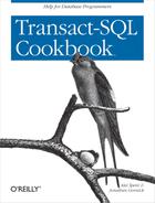
To calculate the confidence interval for a sample, you first need to decide on a required probability. This will be the probability that the mean of the entire population falls within the confidence interval that you compute based on the mean of your sample. You also need to know the mean of your sample and the standard deviation from that sample. Once you have that information, calculate your confidence interval using the following formula:
where:
For example, consider the following data, which you also saw earlier in this chapter:
| 100 cm |
| 100 cm |
| 100 cm |
| 110 cm |
| 115 cm |
| 120 cm |
| 180 cm |
The mean of this data is 117.86, and the standard deviation is 28.56. There are 7 values in the sample, which gives 6 degrees of freedom. The following query, then, yields the corresponding t-distribution value:
SELECT p
FROM T_distribution
WHERE df=6

p
-------
2.447
The value for P, which is our t-distribution value, is 2.447. The confidence interval, then, is derived as follows:
Correlation
A correlation coefficient is a measure of the linear relationship between two samples. It is expressed as a number between -1 to 1, and it tells you the degree to which the two samples are related. A correlation coefficient of zero means that the two samples are not related at all. A correlation coefficient of 1 means that the two samples are fully correlated — every change in the first sample is reflected in the second sample as well. If the correlation coefficient is -1, it means that for every change in the first sample, you can observe the exact opposite change in the second sample. Values in between these extremes indicate varying degrees of correlation. A coefficient of 0.5, for example, indicates a weaker relationship between samples than does a coefficient of 1.0.
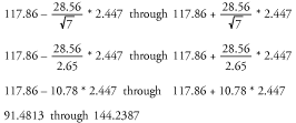
The correlation coefficient for two samples can be calculated using the following formula:
where:
- X
Are the values of the first sample.
- Y
Are the values of the second sample.
- n
Is the number of values in each sample.
Consider the two samples shown in Table 8-1. The first sample represents daily closing stock prices for a particular stock. The second sample represents the value of the corresponding stock-market index over the same set of days. An investor looking at this data might wonder how closely the index tracks the stock price. If the index goes up on any given day, is the stock price likely to go up as well? The correlation coefficient can be used to answer that question.
|
Day |
Stock price |
Index value |
|
1 |
10 |
31 |
|
2 |
18 |
34 |
|
3 |
12 |
35 |
|
4 |
20 |
45 |
|
5 |
10 |
37 |
|
6 |
9 |
39 |
|
7 |
19 |
41 |
|
8 |
13 |
45 |
|
9 |
18 |
47 |
|
10 |
15 |
55 |
To compute the correlation coefficient of the stock price with respect to the index value, you can take the values shown in Table 8-1 and plug them into the formula shown earlier in this section. It doesn’t matter which is X and which is Y. For this example, let X represent the stock price, and Y will represent the index value. The resulting calculation is as follows:
If you put the numbers into the formula, where stock prices represent the X series, index numbers represent the Y series, and number of samples is 10, you get the correlation coefficient of 0.40. The result tells us that the stock price is weakly correlated with the market index.
The formula shown here looks scary at first, and it does take a lot of tedious work to compute a correlation by hand; however, you’ll see that its implementation in SQL is quite straightforward.
Autocorrelation
Autocorrelation is an interesting concept and is very useful in attempting to observe patterns in time-series data. The idea is to calculate a number of correlations between an observed time series and the same time series lagged by one or more steps. Each lag results in a different correlation. The end result is a list of correlations (usually around fifteen), which can be analyzed to see whether the time series has a pattern in it.
Table 8-2 contains the index values that you saw earlier in Table 8-1. It also shows the autocorrelation values that result from a lag of 1, 2, and 3 days. When calculating the first correlation coefficient, the original set of index values is correlated to the same set of values lagged by one day. For the second coefficient, the original set of index values is correlated to the index values lagged by 2 days. The third coefficient is the result of correlating the original set of index values with a 3-day lag.
|
Index values |
Lag 1 |
Lag 2 |
Lag 3 | |
|
1 |
31 | |||
|
2 |
34 |
31 | ||
|
3 |
35 |
34 |
31 | |
|
4 |
45 |
35 |
34 |
31 |
|
5 |
37 |
45 |
35 |
34 |
|
6 |
39 |
37 |
45 |
35 |
|
7 |
41 |
39 |
37 |
45 |
|
8 |
45 |
41 |
39 |
37 |
|
9 |
47 |
45 |
41 |
39 |
|
9 |
55 |
47 |
45 |
41 |
|
10 |
55 |
47 |
45 | |
|
11 |
55 |
47 | ||
|
12 |
55 | |||
|
Correlation |
n/a |
0.6794 |
0.6030 |
0.3006 |
Please note that it’s only possible to calculate a correlation coefficient between two equally sized samples. Therefore, you can use only rows 2 through 9 of Lag 1 when calculating the first correlation coefficient, rows 3 through 10 of Lag 2 for the second, and rows 4 through 11 of the Lag 3 for the third. In real life, you would likely have enough historical data to always use rows 1 through 9.
You can see that the correlation coefficients of the first few lags are declining rather sharply. This is an indication that the time series has a trend (i.e., the values are consistently rising or falling). As you can see, the values of the first three autocorrelations in our example are declining.
The first correlation is the strongest; therefore, the neighboring cases are related significantly. Cases that are 2 and 3 lags apart are still correlated, but not as strongly as the closest cases. In other words, the behavior of neighboring lags is related proportionally to the distance they are apart from each other. If two consecutive cases are increasing, it is probable that the third one will increase as well. The series has a trend. A decreasing autocorrelation is an indicator of a trend, but it has nothing to do with the direction of the trend. Regardless of whether the trend is increasing or decreasing, autocorrelation is still strongest for the closest cases (Lag 1) and weakest for the more distant lags. A sharp increase in the correlation coefficient at regular intervals indicates a cyclical pattern in your data. For example, if you were looking at monthly sales for a toy store, it is likely that every 12th lag you would observe a strong increase in the correlation coefficient due the Christmas holiday sales.
In one of the recipes we show later in this chapter, you’ll see how autocorrelation can be implemented in SQL. In addition, you’ll see how SQL can be used to generate a crude graph of the autocorrelation results quickly.
Moving Averages
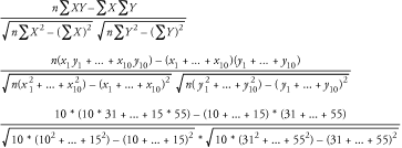
A moving average is used when some kind of smoothing is needed on a set of time-series data. To compute a moving average, you combine every value in the series with some number of preceding values and then compute the average of those values. The result is a series of averages giving a smoother representation of the same data, though some accuracy will be lost because of the smoothing.
Moving averages are commonly used in the financial industry to smooth out daily oscillations in the market price of a stock or other security. Table 8-3 shows a moving average for a stock price over a 10-day period. The left-hand column shows the daily stock price, while the right-hand column shows a 5-day moving average of that price. During the first four days, no moving average is possible, because a 5-day moving average requires values from 5 different days. Thus, the average begins on Day 5.
|
Day |
Stock price |
5-day moving average |
|
1 |
10 |
n/a |
|
2 |
18 |
n/a |
|
3 |
12 |
n/a |
|
4 |
20 |
n/a |
|
5 |
10 |
14.0 |
|
6 |
9 |
13.8 |
|
7 |
19 |
14.0 |
|
8 |
13 |
14.2 |
|
9 |
18 |
17.8 |
|
10 |
15 |
14.8 |
|
11 |
16 |
16.2 |
|
12 |
17 |
15.8 |
|
13 |
15 |
16.2 |
|
14 |
18 |
16.2 |
|
15 |
17 |
16.6 |
You can readily see that the 5-day moving average values in Table 8-3 smooth out most of the wild oscillations in the day-to-day price of the stock. The moving average also makes the very slight upward trend much more clear. Figure 8-1 shows a graph of this same data.
There are a number of different moving averages possible. A simple moving average, such as the one just shown in Table 8-3, represents the mean over a period for every case in the data set. All cases in the period are summed together, and the result is then divided by the number of cases in the period.
It is possible, however, to extend the concept of a moving average further. For example, a simple exponential average uses just two values: the current value and the one before it, but different weights are attached to each of them. A 90% exponential smoothing would take 10% of each value, 90% of each preceding value (from the previous period), and sum the two results together. The list of sums then becomes the exponential average. For example, with respect to Table 8-3, an exponential average for Day 2 could be computed as follows:
(Day 2 * 10%) + (Day 1 * 90%)
= (18 * 10%) + (10 * 90%)
= 1.8 + 9
= 10.8
Another interesting type of moving average is the weighted average, where the values from different periods have different weights assigned to them. These weighted values are then used to compute a moving average. Usually, the more distant a value is from the current value, the less it is weighted. For example, the following calculation yields a 5-day weighted average for Day 5 from Table 8-3.
(Period 5 * 35%) + (Period 4 * 25%) + (Period 3 * 20%)
+ (Period 2 * 15%) + (Period 1 * 5%)

= (10 * 35%) + (20 * 25%) + (12 * 20%) + (18 * 15%) + (10 * 5%)
= 3.5 + 5 + 2.4 + 2.7+ 0.5
= 14.1
As you can readily see, a weighted moving average would tend to favor more recent cases over the older ones.
The Light-Bulb Factory Example
The recipes in this chapter all make use of some sales and quality-assurance data from a hypothetical light bulb factory. This factory is building a quality-support system to store and analyze light-bulb usage data. Managers from every product line send small quantities of light bulbs several times a day to a testing lab. Equipment in the lab then tests the life of each bulb and stores the resulting data into a SQL database. In addition to the bulb-life data, our company also tracks sales data on a monthly basis. Our job is to build queries that support basic statistical analysis of both the bulb-life test data and the sales data.
Bulb-Life Data
Bulb-life test data is stored in the following table. Each bulb is given a unique ID number. Each time a bulb is tested, the test equipment records the bulb’s lifetime in terms of hours.
CREATE TABLE BulbLife (
   BulbId INTEGER,
   Hours INTEGER,
   TestPit INTEGER
)
The test floor is divided into several test pits. In each test pit, a number of light bulbs can be tested at the same time. The table stores the number of hours each light bulb lasted in the testing environment before it burned out. Following is a sampling of data from two test pits:
BulbId      Hours       TestPit
----------- ----------- -----------
1           1085        1
2           1109        1
3           1093        1
4           1043        1
5           1129        1
6           1099        1
7           1057        1
8           1114        1
9           1077        1
10          1086        1
1           1103        2
2           1079        2
3           1073        2
4           1086        2
5           1131        2
6           1087        2
7           1096        2
8           1167        2
9           1043        2
10          1074        2
Sales Data
The marketing department of our hypothetical light-bulb company tracks monthly sales. The sales numbers are stored in a table named BulbSales and are used to analyze the company’s performance. The table is as follows:
CREATE TABLE BulbSales(
   Id INT IDENTITY,
   Year INT,
   Month INT,
   Sales FLOAT
)
The following records represent a sampling of the data from the BulbSales table:
Id           Year         Month       Sales
----------- ----------- ----------- ---------
1           1995        1           9536.0
2           1995        2           9029.0
3           1995        3           8883.0
4           1995        4           10227.0
5           1995        5           9556.0
6           1995        6           9324.0
7           1995        7           10174.0
8           1995        8           9514.0
9           1995        9           9102.0
10          1995        10          9702.0
You can download a file from the book’s web site that contains the complete set of sample sales data used for this chapter’s examples. Figure 8-2 shows a graphical representation of this sales data. The company produces specialized light-bulb equipment and has three major customers. Historically, all three customers generally order three-months worth of supplies every three months and at approximately the same time. The sales record, therefore, shows a peak every three months. A six-month moving average can be used to smooth out this data and show the long-term trend. You see this moving average as the smoother line on the chart.
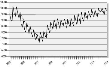
The chart in Figure 8-2 is only an example of the type of statistics that need to be produced from the sales and quality-assurance data. You’ll see how to generate the moving average needed to create this chart in a recipe later in this chapter.
Calculating a Mean
Problem
You want to calculate the average life of light bulbs in a sample, where the sample consists of all bulbs tested in a particular test pit.
Solution
Computing a mean is fairly easy, because the standard SQL function AVG produces the desired result. For example:
SELECT AVG(Hours) Mean
FROM BulbLife
WHERE TestPit=1

Mean
-----------
1089
Discussion
Probably the easiest of all statistics to compute using SQL is the mean. The mean is just a simple average implemented by the standard SQL function AVG. The AVG function is a group function, which means that it operates on a group of rows. In the recipe solution, the group in question consisted of all rows for Test Pit #1. Using the GROUP BY clause, you can extend the query to report the mean bulb life for all test pits. For example:
SELECT TestPit, AVG(hours) Mean
FROM BulbLife
GROUP BY TestPit

TestPit     Mean
----------- -----------
1           1089
2           1093
Using the HAVING clause, you can implement measurement rules requiring that results only be reported for those test pits that have a specified minimum number of measurements available. For example, the following query limits the report to test pits where more than eight light bulbs have been tested:
SELECT TestPit, AVG(hours) Mean
FROM BulbLife
GROUP BY TestPit
HAVING COUNT(*) >= 8
Calculating a Mode
Problem
You want to calculate a modal average of the bulb-life results in your database. Recall from the discussion earlier in this chapter that the mode represents the most frequently occurring value in a sample.
Solution
SQL Server is not equipped with a mode function, so calculating the mode is a bit more difficult than calculating the mean. As the following solution shows, you can calculate the mode using a creative combination of COUNT and TOP:
SELECT TOP 1 COUNT(*) frequency, Hours mode
FROM BulbLife
WHERE TestPit=1
GROUP BY hours
ORDER BY COUNT(*) DESC

frequency   mode
----------- -----------
2           1085
Discussion
Although it appears strange at first, how the query works becomes clear once you think about the basic definition for mode. A mode is the value that occurs most frequently in an observed sample. You can begin by writing a query to group values together:
SELECT Hours
FROM BulbLife
WHERE TestPit=1
GROUP BY hours

hours
-----------
1043
1057
1077
1085
1093
1099
1109
1114
1129
Next, add the COUNT function to the query to include a count of each distinct value with the query’s results:
SELECT COUNT(*) frequency, Hours
FROM BulbLife
WHERE TestPit=1
GROUP BY Hours

frequency   Hours
----------- -----------
1           1043
1           1057
1           1077
2           1085
1           1093
1           1099
1           1109
1           1114
1           1129
Finally, use an ORDER BY clause to put the results in descending order by frequency, so that the most frequently occurring value is listed first. Then, use the TOP 1 syntax in your SELECT clause to limit the results to the first row. The hours value in that first row will be the mode.
What happens when you have more than one mode in the observed sample and you need to report all such values? In our hypothetical bulb-life data, the mode for Test Pit #1 is 1085, while the mode for Test Pit #2 is 1043. For both modes, the occurrence count is 2. If you want the mode for all light bulbs, regardless of test pit, then both values should be returned. The following query shows one way to deal with this:
SELECT COUNT(*) frequency, Hours mode FROM BulbLife
GROUP BY Hours
HAVING COUNT(*)>= ALL(
   SELECT COUNT(*)
   FROM BulbLife
   GROUP BY Hours)

frequency   mode
----------- -----------
2           1043
2           1085
The subquery that you see in this example returns a list of all occurrence counts for all distinct values in the BulbLife table. It follows, logically, that one of those counts will represent a maximum. The HAVING clause in the outer query specifies that the occurrence count be greater than or equal to all values returned by the subquery, which, in effect, restricts the results to only those rows with an occurrence count that equals the maximum occurrence count.
Be aware that mode is a weak statistic. The mode can be useful if you know the distribution and the nature of the sample, but it can easily be altered by adding a few cases with extreme values. For example, let’s say that we get 2 additional bulbs with a duration of 1129 hours. The mode is then 1129, which is misleading information, since all other bulbs lasted for much shorter periods.
Calculating a Median
Problem
You want to calculate the median bulb life for all bulbs that have been tested. From the discussion earlier in this chapter, you should recognize that the median bulb life represents the case where the number of bulbs with shorter lives is equivalent to the number of bulbs with longer lives.
Solution
To calculate the median of the light-bulb test results, use the following query:
SELECT x.Hours median
FROM BulbLife x, BulbLife y
GROUP BY x.Hours
HAVING
   SUM(CASE WHEN y.Hours <= x.Hours
      THEN 1 ELSE 0 END)>=(COUNT(*)+1)/2 AND
   SUM(CASE WHEN y.Hours >= x.Hours
      THEN 1 ELSE 0 END)>=(COUNT(*)/2)+1

median
-----------
1086
Discussion
This query follows the definition of the median very closely and uses the solution published several years ago by David Rozenshtein, Anatoly Abramovich, and Eugene Birger. Their solution is still regarded as one of the classical solutions to the problem of finding the median value in a sample. To understand their solution, it helps to look at the query in two phases. First, you have a GROUP BY query that returns the number of bulbs for each distinct lifetime. The following is a modified version of the first part of the solution query that returns the occurrence count corresponding to each distinct bulb-life value:
SELECT COUNT(*) occurrences, x.Hours xhours
FROM BulbLife x, BulbLife y
GROUP BY x.Hours

occurrences xhours
----------- -----------
40          1043
20          1057
20          1073
20          1074
20          1077
20          1079
40          1085
20          1086
20          1087
20          1093
20          1096
20          1099
20          1103
20          1109
20          1114
20          1129
20          1131
20          1167
Because these results represent a self-join of the BulbLife table with itself, each group represents a number of detail rows equivalent to the number of rows in the sample. The two groups of 40 occurrences each exist because the data contains 2 cases with values of 1043 and 2 cases with values of 1085. The detail for the 1086 group is as follows:
xhours      yhours
----------- -----------
1086        1043
1086        1043
1086        1057
1086        1073
1086        1074
1086        1077
1086        1079
1086        1085
1086        1085
1086        1086
1086        1087
1086        1093
1086        1096
1086        1099
1086        1103
1086        1109
1086        1114
1086        1129
1086        1131
1086        1167
The question now is whether the value 1086 represents the median. To determine that, follow these steps:
Count the cases where the y.hours value is less than or equal to the x.hours value.
Count the cases where the x.hours value is less than or equal to the y.hours value.
Compare the two results. If they are equal, then 1086 is the median value.
The HAVING clause in our solution query performs the counts for steps 1 and 2 using the following two invocations of the SUM function combined with a CASE statement:
SUM(CASE WHEN y.Hours <= x.Hours
   THEN 1 ELSE 0 END)
SUM(CASE WHEN y.Hours >= x.Hours
   THEN 1 ELSE 0 END)
In our example, the values for these 2 sums work out to 10 and 11, respectively. Plug these two values in for the two SUM expressions in the HAVING clause, and you have the following:
10 >= (COUNT(*)+1)/2 AND
11 >= (COUNT(*)/2)+1
At this point, the two COUNT expressions deserve some additional explanation. They have been carefully crafted to allow us to derive a median, even in cases where we have an even number of values in the sample. Let’s step back for a moment, and assume that our sample contained 21 values, instead of the 20 that it does contain. If that were the case, the two COUNT expressions would evaluate as follows:
(COUNT(*)+1)/2         (COUNT(*)/2)+1
(21+1)/2               (21/2)+1
22/2                   10+1
11                     11
Tip
In SQL Server, 21/2 represents an integer division and, hence, yields an integer value of 10 as the result.
Whenever you have an odd number of values in the sample, the two expressions will yield the same result. Given an even number, however, the first expression will yield a result that is one less than the other. Here is how the HAVING expression works out for the data in our example:
10 >= (20+1)/2 AND
11 >= (20/2)+1

10 >= 10 AND
11 >= 11
For the case where x.Hours = 1086, both expressions are true, so 1086 is returned as the median value. In actual fact, because we have an even number of values, there are 2 candidates for the median: 1086 and 1087. The value 1086 has 9 values below it and 10 above it. The value for 1087 has 10 values below it and 9 above it. Due to how we’ve written the COUNT expressions, our solution query arbitrarily returns the lower value as the median.
It’s possible to use a slightly modified version of our solution query to return the financial median. Recall, from earlier in this chapter, that in the case of an even number of values, the financial median represents the mean of the two inner neighbors. With respect to our example, that would be the mean of 1086 and 1087, which works out to 1086.5. Use the following query to calculate the financial median:
SELECT
   CASE WHEN COUNT(*)%2=1
        THEN x.Hours
        ELSE (x.Hours+MIN(CASE WHEN y.Hours>x.Hours
                               THEN y.Hours
                          END))/2.0
   END median
FROM BulbLife x, BulbLife y
GROUP BY x.Hours
HAVING
   SUM(CASE WHEN y.Hours <= x.Hours
      THEN 1 ELSE 0 END)>=(count(*)+1)/2 AND
   SUM(CASE WHEN y.Hours >= x.Hours
      THEN 1 ELSE 0 END)>=(count(*)/2)+1
The basic query remains the same, the only difference being in the SELECT statement’s column list. If there is an odd number of cases, the median is reported directly as the x.Hours value. However, if the number of cases is even, the smallest y.Hoursvalue that is higher than the chosen x.Hours value is identified. This value is then added to the x.Hours value. The result is then divided by 2.0 to return the mean of those two values as the query’s result.
The original query reported only the lesser of the two values that were in the middle of the sample. The added logic in the SELECT clause for the financial-median causes the mean of the two values to be calculated and reported. In our example, the result is the following:
median
-------------------
1086.5
After you run the query to obtain a financial median, you’ll get a warning like this:
Warning: Null value eliminated from aggregate.
This is an important warning, because it’s a sign that our query is working correctly. We did not want to write an ELSE clause for the CASE statement inside the MIN function. Because if we wrote such an ELSE clause and had it return a 0, the result of the MIN function would always be 0, and, consequently, the financial-median calculation would always be wrong for any sample with an even number of values.
Calculating Standard Deviation, Variance, and Standard Error
Problem
You want to calculate both the standard deviation and the variance of a sample. You also want to assess the standard error of the sample.
Solution
Use SQL Server’s built-in STDEV, STDEVP, VAR, and VARP functions for calculating standard deviation and variance. For example, the following query will return the standard deviation and variance for the sample values from each of the test pits:
SELECT TestPit, VAR(Hours) variance, STDEV(Hours) st_deviation
FROM BulbLife
GROUP BY TestPit

TestPit variance  st_deviation
------- --------- ------------
1       672.99    25.94
2       1173.66   34.26
To get the standard error of the sample, simply use the following query, which implements the formula for standard error shown earlier in this chapter:
SELECT AVG(Hours) mean, STDEV(Hours)/SQRT(COUNT(*)) st_error
FROM BulbLife

mean        st_error
----------- ----------
1091        6.64
Discussion
Since SQL Server provides functions to calculate standard deviation and variance, it is wise to use them and not program your own. However, be careful when you use them. You need to know whether the data from which you calculate the statistics represents the whole population or just a sample. In our example, the table holds data for just a sample of the entire population of light bulbs. Therefore, we used the STDEV and VAR functions designed for use on samples. If your data includes the entire population, use STDEVP and VARP instead.
Building Confidence Intervals
Problem
You want to check to see whether the calculated sample statistics could be reasonably representative of the population’s statistics. With respect to our example, assume that a light bulb’s declared lifetime is 1100 hours. Based on a sample of lifetime tests, can you say with 95% probability that the quality of the production significantly differs from the declared measurement? To answer this question, you need to determine whether the confidence interval around the mean of the sample spans across the declared lifetime. If the declared lifetime is out of the confidence interval, then the sample mean does not represent the population accurately, and we can assume that our declared lifetime for the light bulbs is probably wrong. Either the quality has dropped and the bulbs are burning out more quickly, or quality has risen, causing the bulbs to last longer than we claim.
Solution
The solution is to execute a query that implements the calculations described earlier for computing a confidence interval. Recall that the confidence interval was plus or minus a certain amount. Thus, the following solution query computes two values:
SELECT
   AVG(Hours)-STDEV(Hours)/SQRT(COUNT(*))*MAX(p) in1,
   AVG(Hours)+STDEV(Hours)/SQRT(COUNT(*))*MAX(p) in2
FROM BulbLife, T_distribution
WHERE df=(
   SELECT
      CASE WHEN count(*)<=29
      THEN count(*)-1
      ELSE -1 END FROM BulbLife)

in1      in2
-------- --------
1077.11  1104.89
Based on the given sample, we cannot say that the quality of production has significantly changed, because the declared value of 1100 hours is within the computed confidence interval for the sample.
Discussion
The solution query calculates the mean of the sample and adds to it the standard error multiplied by the t-distribution coefficient from the T_distribution table. In our sample, the degree of freedom is the number of cases in the sample less 1. The CASE statement ensures that the appropriate index is used in the T_distribution table. If the number of values is 30 or more, the CASE statement returns a -1. In the T_distribution table, the coefficient for an infinite number of degrees of freedom is identified with a -1 degree of freedom value. Expressions in the SELECT clause of the solution query calculate the standard deviation, expand it with the coefficient from the T_distribution table, and then calculate the interval around the mean.
This example is interesting, because it shows you how to refer to a table containing coefficients. You could retrieve the coefficient separately using another query, store it in a local variable, and then use it in a second query to compute the confidence interval, but that’s less efficient than the technique shown here where all the work is done using just one query.
Calculating Correlation
Problem
You want to calculate the correlation between two samples. For example, you want to calculate how similar the light-bulb sales patterns are for two different years.
Solution
The query in the following example uses the formula for calculating correlation coefficients shown earlier in this chapter. It does this for the years 1997 and 1998.
SELECT
   (COUNT(*)*SUM(x.Sales*y.Sales)-SUM(x.Sales)*SUM(y.Sales))/(
   SQRT(COUNT(*)*SUM(SQUARE(x.Sales))-SQUARE(SUM(x.Sales)))*
   SQRT(COUNT(*)*SUM(SQUARE(y.Sales))-SQUARE(SUM(y.Sales))))
   correlation
FROM BulbSales x JOIN BulbSales y ON x.month=y.month
WHERE x.Year=1997 AND y.Year=1998

correlation
-----------------------------------------------------
0.79
The correlation calculated is 0.79, which means that the sales patterns between the two years are highly correlated or, in other words, very similar.
Discussion
The solution query implements the formula shown earlier in the chapter for calculating a correlation coefficient. The solution query shown here is an example of how you implement a complex formula directly in SQL. To aid you in making such translations from mathematical formulas to Transact-SQL expressions, Table 8-4 shows a number of mathematical symbols together with their corresponding Transact-SQL functions.
|
Symbol |
Formula |
Description |
|
|a| |
ABS(a) |
Absolute value of a |
|
ea |
EXP(a) |
Exponential value of a |
|
a2 |
SQUARE(a) |
Square of a |
|
an |
POWER(a,n) |
nth power of a |
|
n |
COUNT(*) |
Sample size |
|
|
SQRT(a) |
Square root of a |
|
|
SUM(a) |
Sum of all cases in a sample |
|
or
|
AVG(a) |
Average of all cases in a sample — the mean |
|
s |
STDDEV(x) |
Standard deviation of a sample |
|
|
STDDEVP(x) |
Standard deviation of a population |
|
s2 |
VAR(x) |
Variance of a sample |
|
|
VARP(X) |
Variance of a population |
To write the query shown in this recipe, take the formula for correlation coefficient shown earlier in this chapter, and use the Table 8-4 to translate the mathematical symbols in that formula into SQL functions for your query.
Exploring Patterns with Autocorrelation
Problem
You want to find trend or seasonal patterns in your data. For example, you wish to correlate light-bulb sales data over a number of months. To save yourself some work, you’d like to automatically correlate a number of samples.
Solution
Use the autocorrelation technique described earlier in this chapter, and print a graphical representation of the results. You need to calculate up to 15 correlations of the light-bulb sales data. 15 is a somewhat arbitrary number. In our experience, we rarely find a gain by going beyond that number of correlations. For the first correlation, you want to compare each month’s sales data with that from the immediately preceding month. For the second correlation, you want to compare each month’s sales data with that from two months prior. You want this pattern to repeat 15 times, with the lag increasing each time, so that the final correlation compares each month’s sales data with that from 15 months prior. You then wish to plot the results in the form of a graph.
Because you want to compute 15 separate correlations, you need to do more than just join the BulbSales table with itself. You actually want 15 such joins, with the lag between months increasing each time. You can accomplish this by joining the BulbSales table with itself, and then joining those results with the Pivot table. See the Pivot table recipe in Chapter 1 for an explanation of the Pivot table.
After you create the necessary Pivot table, you can use the query shown in the following example to generate and graph the 15 correlations that you wish to see:
SELECT
   p.i lag, STUFF( STUFF(SPACE(40),
      CAST(ROUND((COUNT(*)*SUM(x.Sales*y.Sales)-
         SUM(x.Sales)*SUM(y.Sales))/
         (SQRT(COUNT(*)*SUM(SQUARE(x.Sales))-SQUARE(SUM(x.Sales)))*
          SQRT(COUNT(*)*SUM(SQUARE(y.Sales))-SQUARE(SUM(y.Sales))))*
          20,0)+20 AS INT),1,'*'),20,1,'|') autocorrelation
FROM BulbSales x, BulbSales y, Pivot p
WHERE x.Id=y.Id-p.i AND p.i BETWEEN 1 AND 15
GROUP BY p.i
ORDER BY p.i

lag         autocorrelation
----------- ----------------------------------------
1                              |              *
2                              |             *
3                              |                  *
4                              |            *
5                              |           *
6                              |               *
7                              |         *
8                              |        *
9                              |            *
10                             |      *
11                             |    *
12                             |         *
13                             |   *
14                             | *
15                             |      *
You can see from this graph that, as the lag increases, the correlation drops towards 0. This clearly indicates a trend. The more distant any two cases are, the less correlated they are. Conversely, the closer any two cases are, the greater their correlation.
You can make another observation regarding the 3rd, 6th, 9th, 12th, and 15th lags. Each of those lags shows an increased correlation, which indicates that you have some sort of seasonal pattern that is repeated every three periods. This is true. If you look at the sample data, you will see that sales results increase significantly every three months.
Discussion
This code demonstrates how you can extend a correlation, or any other kind of formula, so that it is calculated several times on the same data. In our solution, the first 15 correlation coefficients are calculated from the sample. Each coefficient represents the correlation between the sample and the sample lagged by one or more steps. We use the Pivot table to generate all the lagged data sets. Let’s look at a simplified version of the query that doesn’t contain the plotting code:
SELECT
   p.i lag,
   (COUNT(*)*SUM(x.Sales*y.Sales)-SUM(x.Sales)*SUM(y.Sales))/
      (SQRT(COUNT(*)*SUM(SQUARE(x.Sales))-SQUARE(SUM(x.Sales)))*
       SQRT(COUNT(*)*SUM(SQUARE(y.Sales))-SQUARE(SUM(y.Sales))))
       autocorrelation
FROM BulbSales x, BulbSales y, Pivot p
WHERE x.Id=y.Id-p.i AND p.i BETWEEN 1 AND 15
GROUP BY p.i
ORDER BY p.i
When you execute this query, the first few lines of the result should look like this:
lag         autocorrelation
----------- -------------------
1           0.727
2           0.703
3           0.936
4           0.650
5           ...
The code in the SELECT clause that calculates the correlations is the
same as that used in the earlier recipe for calculating a single
correlation. The difference here is that we define the matching
months differently. Since our research spans a period greater than
one year, we cannot match months anymore. Instead, we have to use the
period index. Hence, the WHERE clause specifies the condition,
x.id=y.id-p.i. For pivot value 1, each x value
will be matched with the preceding y value. For pivot value 2, each x
value will be matched by the y value from two periods in the past.
This pattern continues for all 15 lags.
For every calculation, the data must be lagged. We use the Pivot table to generate 15 groups, where the group index is also used as a lag coefficient in the WHERE clause. The result is a list of correlation coefficients, each calculated for a combination of the sample data and correspondingly lagged sampled data.
Now that you understand the use of the Pivot table to generate the 15 lags that we desire, you can return your attention to our original query. To make use of autocorrelation, we need to print the data in a graphical format. We do that by printing an asterisk (*) in the autocorrelation column of the output. The greater the correlation value, the further to the right the asterisk will appear. The following query highlights the Transact-SQL expression that we use to plot the results. To simplify things, we use the pseudovariable correlation coefficient (CORR) to represent that part of the code that calculates the correlation values.
SELECT
   p.i lag, STUFF( STUFF(SPACE(40),
      CAST(ROUND(CORR*20,0)+20 AS INT),1,'*'),20,1,'|')
      autocorrelation
FROM BulbSales x, BulbSales y, Pivot p
WHERE x.Id=y.Id-p.i AND p.i BETWEEN 1 AND 15
GROUP BY p.i
ORDER BY p.i
You have to look at this expression from the inside out. The CORR is multiplied by 20, and any decimal digits are rounded off. This translates our correlation coefficient values from the range -1 to 1 into the range -20 to 20. We add 20 to this result to shift those values into the range 0 to 40. For example, -0.8 is translated into 4, and 0.7 is translated into 34. Since all the values are positive, we can place each asterisk into its correct relative position simply by preceding it with the number of spaces indicated by our result.
The SPACE function in our expression generates a string containing 40 spaces. The STUFF function is then used to insert an asterisk into this string of blanks. After that, the outermost STUFF function inserts a vertical bar (|) character to indicate the middle of the range. This allows us to see easily when a correlation coefficient is positive or negative. Any asterisks to the left of the vertical bar represent negative coefficients. If the coefficient came out as zero, it would be overwritten by the vertical bar.
Using a Simple Moving Average
Problem
You want to develop a moving-average tool for your analysis. For example, you want to smooth out monthly deviations in light-bulb sales using a six-month moving average. This will allow you to get a good handle on the long-term trend.
Solution
Calculating a moving average turns out to be a fairly easy task in SQL. With respect to the example we are using in this chapter, the query shown in the following example returns a six-month moving average of light-bulb sales:
SELECT x.Id, AVG(y.Sales) moving_average
FROM BulbSales x, BulbSales y
WHERE x.Id>=6 AND x.Id BETWEEN y.Id AND y.Id+5
GROUP BY x.Id
ORDER BY x.Id

id          moving_average
----------- ---------------
6           9425.83
7           9532.17
8           9613.00
9           9649.50
10          9562.00
11          9409.33
12          9250.67
13          9034.83
14          8812.83
15          8609.83
16          8447.83
17          8386.33
18          ...
The query shown in this example was used to generate the chart shown earlier in this chapter in Figure 8-2. Please refer to that chart to see the graphical representation of the query results that you see here.
Discussion
In our solution, the moving average is calculated through the use of a self-join. This self-join allows us to join each sales record with itself and the sales records from the preceding six periods. For example:
SELECT x.Id xid, y.Id yid, y.Sales
FROM BulbSales x, BulbSales y
WHERE x.Id>=6 AND x.Id BETWEEN y.Id AND y.Id+5
ORDER BY x.Id

xid         yid         Sales
----------- ----------- -----------------------------------------------------
6           1           9536.0
6           2           9029.0
6           3           8883.0
6           4           10227.0
6           5           9556.0
6           6           9324.0
7           2           9029.0
7           3           8883.0
7           4           10227.0
7           5           9556.0
7           6           9324.0
7           7           10174.0
8           3           8883.0
8           4           10227.0
8           5           9556.0
8           6           9324.0
8           7           10174.0
8           8           9514.0
To compute a 6-month moving average, we need at least 6 months worth
of data. Thus, the WHERE clause specifies
x.Id>=6. Period 6 represents the first period
for which we can access 6 months of data. We cannot compute a 6-month
moving average for periods 1 through 5.
The WHERE clause further specifies x.Id BETWEEN y.Id AND
y.Id+5. This actually represents the join condition and
results in each x row being joined with the corresponding y row, as
well as the five prior y rows. You can see that for
x.Id=6, the query returns sales data from periods
1 through 6. For x.Id=7, the query returns sales
data from periods 2 through 7. For x.Id=8, the
window shifts again to periods 3 through 8.
To compute the moving average, the Id value from the first table is used as a reference — the results are grouped by the x.Id column. Each grouping represents six rows from the second table (aliased as y), and the moving average is computed by applying the AVG function to the y.Sales column.
Extending Moving Averages
Problem
You want to calculate an extended moving average such as is used in the financial industry. In particular, you want to calculate exponential and weighted moving average. Let’s say that by looking at a chart of light-bulb sales, you find that they closely mimic the company’s stock-price data from the stock exchange. As a possible investor, you want to calculate some of the same moving averages that financial analysts are using.
Solution
To calculate a 90% exponential moving average, you begin with the same basic moving-average framework shown in the previous recipe. The difference is how you calculate the average. Recall that a 90% exponential moving average gives 90% of the importance to the previous value and only 10% of the importance to the current value. You can use a CASE statement in your query to attach the proper importance to the proper occurrence. The following example shows our solution query:
SELECT x.Id,
   SUM(CASE WHEN y.Id=x.Id
            THEN 0.9*y.Sales
            ELSE 0.1*x.Sales END) exponential_average
FROM BulbSales x, BulbSales y
WHERE x.Id>=2 AND x.Id BETWEEN y.Id AND y.Id+1
GROUP BY x.Id
ORDER BY x.Id

id          exponential_average
----------- --------------------
2           9029.0
3           8883.0
4           10227.0
5           9556.0
6           9324.0
7           10174.0
8           9514.0
9           9102.0
10          ...
The framework for calculating an exponential moving average remains the same as for calculating a simple moving average; the only difference is in the part of the query that actually calculates the average. In our solution, the CASE statement checks which y row is currently available. If it is the latest one, the code places a 90% weight on it. Only a 10% weight is given to the preceding value. The SUM function then sums the two adjusted values, and the result is returned as the exponential weighted average for the period.
As an example of how to extend this concept, think about calculating a six-month weighted moving average where each period has an increasing weight as you move towards the current point. The query in the following example shows one solution to this problem. As you can see, the framework again remains the same. The average calculation has just been extended to include more cases.
SELECT x.Id,
   SUM(CASE WHEN x.Id-y.Id=0 THEN 0.28*y.Sales
            WHEN x.Id-y.Id=1 THEN 0.23*y.Sales
            WHEN x.Id-y.Id=2 THEN 0.20*y.Sales
            WHEN x.Id-y.Id=3 THEN 0.14*y.Sales
            WHEN x.Id-y.Id=4 THEN 0.10*y.Sales
            WHEN x.Id-y.Id=5 THEN 0.05*y.Sales
        END)weighted_average
FROM BulbSales x, BulbSales y
WHERE x.Id>=6 AND x.Id BETWEEN y.Id AND y.Id+6
GROUP BY x.Id
ORDER BY x.Id

Id          weighted_average
----------- -----------------
6           9477.31
7           9675.97
8           9673.43
9           9543.89
10          9547.38
11          9286.62
12          9006.14
13          8883.86
14          8642.43
15          ...
The CASE statement in this example checks to see how far the current y row is from the x row used as a reference and adjusts the value accordingly using a predefined coefficient. You can easily extend the calculation to include ranges, or even dynamic coefficient calculations, depending on your needs. You just need to be careful that the sum of the coefficients is 1. Your weights need to add up to 100%, otherwise your results might look a bit strange.
Discussion
There is a small difference between the two averages shown in this recipe. When calculating an exponential moving average, you assign a proportion of the weight, expressed as a percentage, to each value used in computing the average. Exponential moving averages are calculated using two cases — the current case and its predecessor. When calculating a weighted moving average, you assign weight in terms of multiples to a value in the average. There is no limit to the number of cases that you can use in a weighted moving-average calculation. Exponential moving averages are an often-used special case of weighted moving averages.