
Earth Science
Figures
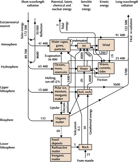
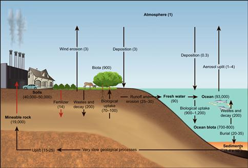
Figure 18.1 Schematic diagram of the Earth’s energy flows without anthropogenic interference. The flows are in TW (1012 W). Numbers in parentheses are uncertain or rounded off. Sørensen, Bent. 2011. Renewable Energy (Fourth Edition), (Boston, Academic Press).
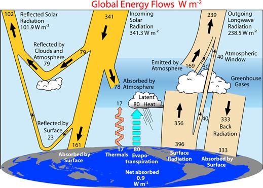
Figure 18.2 The global annual mean Earth’s energy budget for the March 2000 to May 2004 period (W m–2). The broad arrows indicate the schematic flow of energy in proportion to their importance. Source: Trenberth, Kevin E., John T. Fasullo, Jeffrey Kiehl. 2009. Earth’s Global Energy Budget, Bulletin of the American Meteorological Society, Volume 90, Issue 3, 311-323.
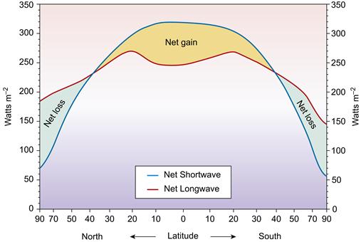
Figure 18.3 Earth’s radiation balance. From 0 - 30° latitude North and South incoming solar radiation exceeds outgoing terrestrial radiation and a surplus of energy exists. The reverse holds true from 30 - 90° latitude North and South and these regions have a deficit of energy. Surplus energy at low latitudes and a deficit at high latitudes results in energy transfer from the equator to the poles. It is this meridional transport of energy that causes atmospheric and oceanic circulation. If there were no energy transfer the poles would be 25° Celsius cooler, and the equator 14° Celsius warmer. Source: Adapted from Pidwirny, Michael, Energy balance of Earth, Encyclopedia of Earth, <http://www.eoearth.org/article/Energy_balance_of_Earth>.
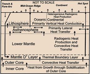
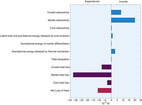
Figure 18.4 Schematic representation of heat sources and transport in the Earth and heat loss at the surface. The two primary heat sources are radiogenic heat production (~80%) and secular cooling of the earth (~20%). Lithospheric extension, magmatism, and upward water flow increase surface heat flow by advection. Subduction, compression, and downward water flow decrease surface heat flow unless accompanied by magmatism. Changes in surface temperature associated with climate change, erosion, and sedimentation cause transient changes in surface heat flow. Source: Morgan, Paul. 2003. Heat Flow, In: Robert A. Meyers, Editor-in-Chief, Encyclopedia of Physical Science and Technology (Third Edition), (New York, Academic Press), Pages 265-278.
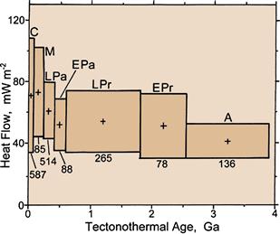
Figure 18.5 Average continental heat flow versus tectonothermal age in billions of years (Ga), the age of the last major tectonic or magmatic event at the heat flow site. Data are grouped in geological age ranges: C–Cenozoic, M–Mesozoic, LPa–Late Paleozoic, EPa–Early Paleozoic, LPr–Late Proterozoic, EPr–Early Proterozoic, A–Archean. Crosses are plotted at the mean heat flow and the midpoint of the age range. Box widths indicate age range and box heights indicate ± one standard deviation of the heat flow data about the mean. Numbers below the boxes indicate the number of data in each group. Source: Morgan, Paul. 2003. Heat Flow, In: Robert A. Meyers, Editor-in-Chief, Encyclopedia of Physical Science and Technology (Third Edition), (New York, Academic Press), Pages 265-278.
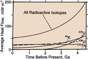
Figure 18.6 Average surface heat flow in mW m−2 from the Earth generated from each of the major radiogenic heat producing isotopes, and all of the isotopes, as a function of time before present in billions of years (Ga). An additional 20% of heat flow from the modern Earth is estimated to come from gradual cooling of the earth. Source: Morgan, Paul. 2003. Heat Flow, In: Robert A. Meyers, Editor-in-Chief, Encyclopedia of Physical Science and Technology (Third Edition), (New York, Academic Press), Pages 265-278.
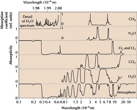
Figure 18.7 Spectral absorption efficiency of selected gaseous constituents of the atmosphere, and for the atmosphere as a whole (bottom). Source: Sørensen, Bent. 2011. Renewable Energy (Fourth Edition), (Boston, Academic Press).
Figure 18.8 Schematic summary of the water cycle. Source: Sørensen, Bent. 2011. Renewable Energy (Fourth Edition), (Boston, Academic Press).
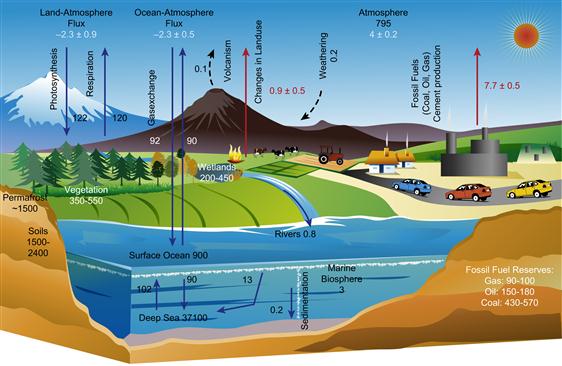
Figure 18.9 The global carbon cycle. Source: Adapted from Intergovernmental Panel on Climate Change.
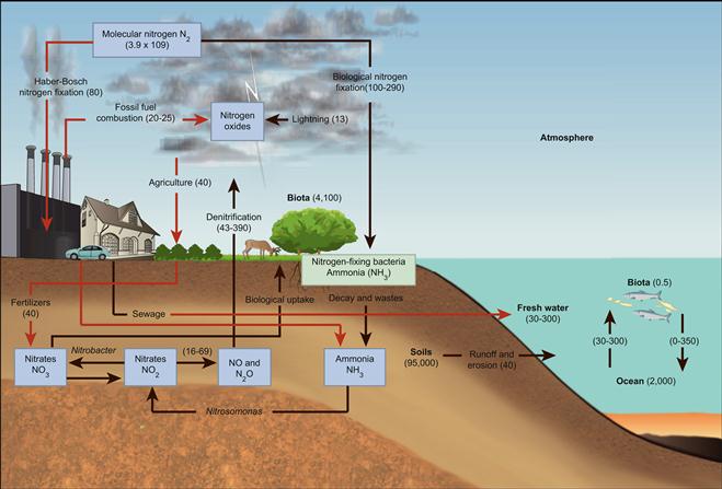
Figure 18.10 The global nitrogen cycle. Source: Adapted from Data from Kaufmann, Robert K. and Cleveland, Cutler J. 2007. Environmental Science (McGraw-Hill, Dubuque, IA).

Figure 18.11 The global methane cycle. Source: Adapted from Intergovernmental Panel on Climate Change.
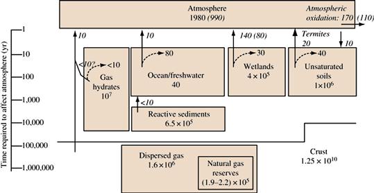
Figure 18.12 Reservoirs (Tg CH4 or Tg C) and fluxes (Tg CH4 yr−1) of the natural, pre-industrial methane carbon subcycle. Values for glacial periods, where available, are shown in parentheses. Values for reactive sediments, wetlands, unsaturated soils, and crustal reservoirs represent organic carbon that might be converted to methane, and are all given as Tg C. The vertical bar on the left shows the approximate time (in years) necessary for the different reservoirs to affect the atmosphere. Estimates of methane consumption within reservoirs are shown as dashed arrows. Gross production of methane within a reservoir can be calculated by adding the flux to the atmosphere and the consumption value. The flux and consumption values are rounded to the nearest 10 Tg CH4 or Tg C. Source: Sundquist, E.T. and K. Visser. 2003. The Geologic History of the Carbon Cycle, In: Heinrich D. Holland and Karl K. Turekian, Editor(s)-in-Chief, Treatise on Geochemistry, (Oxford, Pergamon), Pages 425-472.
Tables
Table 18.1
Energy in the global atmosphere
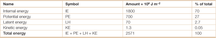
Source: Adapted from Hartmann, Dennis L. 1994. Global Physical Climatology, (San Diego, Academic Press).
Table 18.2
Comparison of global energies in the solid Earth
| Source of Energy | Energy (1030 J) | |
| 1 | Accretion of a homogeneous mass | 219.0 |
| 2 | Core separation less strain energy | 13.9 |
| 3 | Inner core formation | 0.09 |
| 4 | Mantle differentiation | 0.03 |
| 5 | Elastic strain | 15.8 |
| 6 | Radiogenic heat in 4.5 × 10⁹ years | 7.6 |
| 7 | Residual stored heat | 13.3 |
| 8 | Heat loss in 4.5 × 10⁹ years | 13.4 |
| 9 | Present rotational energy | 0.2 |
| 10 | Tidal dissipation in 4.5 × 10⁹ years | ~1.1 |
The first four entries give gravitational energy release with the resulting elastic strain energies subtracted. Strain enegy is listed seperately, so that gravitational energy is the sum of items 1-5. Tidal dissipation occurs mainly in the sea and does not influence the thermal state of the solid Earth.
Source: Adapted from Stacey, F.D. and P.M. Davis. 2008. Physics of the Earth, 4th ed., (Cambridge University Press, Cambridge, UK).
Table 18.3
Surface components of the annual mean energy budget for the Earth
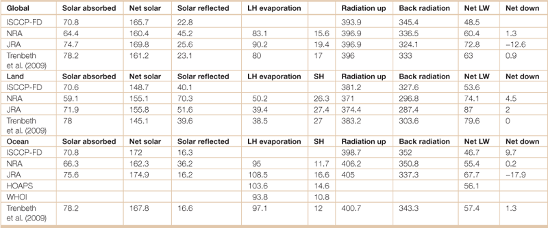
Surface components of the annual mean energy budget for the globe, global land, and global ocean, except for atmospheric solar radiation absorbed (Solar absorb, left column), for the clouds and the earth’s radiant energy system period of Mar 2000 to May 2004 (W m–2). Included are the solar absorbed at the surface (Solar down), reflected solar at the surface (Solar reflected), surface latent heat from evaporation (LH evaporation), sensible heat (SH), LW radiation up at the surface (Radiation up), LW downward radiation to the surface (Back radiation), net LW (Net LW), (net long wave) and net energy absorbed at the surface (NET down). ISCCP = International Satellite Cloud Climatology Project; NRA = reanalysis of NCAR (National Centers for Atmospheric Research) and NCEP (National Center for Environmental Prediction); JRA = Japanese reanalysis; HOAPS = Hamburg Ocean Atmosphere Parameters and Fluxes from Satellite Data; WHOI = Woods Hole Oceanographic Institution. HOAPS version 3 covers 80°S–80°N and is for 1988 to 2005. For the ocean, the ISCCP-FD is combined with HOAPS to provide a NET value.
Source: Adapted from Trenberth, Kevin E., John T. Fasullo, Jeffrey Kiehl, 2009: Earth’s global energy budget. Bull. Amer. Meteor. Soc., 90, 311–323.
Table 18.4
Annual energy balance of the oceans and continents (W m−2)
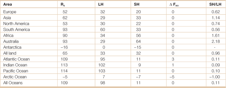
Rs = net radiative flux at surface; LH = latent heat flux; SH = sensible heat flux; ΔFeo = horizontal flux below surface.
Source: Adapted from Hartmann, Dennis L. 1994. Global Physical Climatology, (San Diego, Academic Press).
Table 18.5
Estimates of global primary exergy sources
| Primary exergy source | Magnitude MJ/yr |
| Solar radiationa | 3.33 × 10¹⁸ to 3.83 × 10¹⁸ |
| Moon gravity | 7.6E × 1013 to 1.17 × 10¹⁴ |
| Geothermal heat | 9.78 × 10¹⁴ to 1.98 × 10¹⁵ |
aThe exergy input of net solar radiation into the Earth system.
Source: Adapted from Liao, Wenjie, Reinout Heijungs, Gjalt Huppes. 2012. Natural resource demand of global biofuels in the Anthropocene: A review, Renewable and Sustainable Energy Reviews, Volume 16, Issue 1, Pages 996–1003.
Table 18.6
Physical properties of air at various temperatures
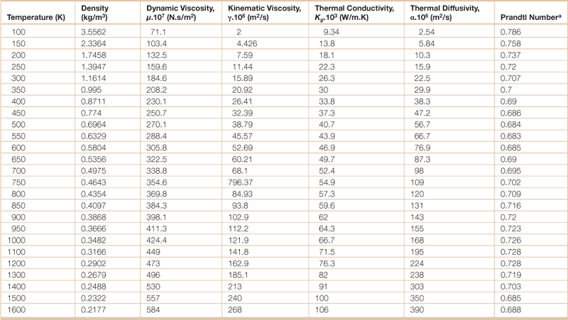
aThe ratio of momentum diffusivity (kinematic viscosity) to thermal diffusivity.
Table 18.7
Key constituents of air in the troposphere and stratosphere
| Constituent | Fraction by volume in (or relative to) dry air | Significant absorption bands |
| N2 | 78.10% | --- |
| O2 | 20.90% | UV-C, MW near 60 and 118 |
| GHz, weak bands in VIS and IR | ||
| H2O | (0–2%) | numerous strong bands throughout IR; also in MW, especially near 183 GHz |
| Ar and other inert gases | 0.94% | --- |
| CO2 | 370 ppm | near 2.8, 4.3, and 15 µm |
| CH4 | 1.7 ppm | near 3.3 and 7.8 µm |
| N2O | 0.35 ppm | 4.5, 7.8, and 17 µm |
| CO | 0.07 ppm | 4.7 µm (weak) |
| O3 | ~10−8 | UV-B, 9.6 µm |
| CFCl3, CF2Cl2, etc | ~10−10 | IR |
Source: Adapted from Petty, Grant. 2006. Atmospheric Radiation (Second edition), (Madison, Wisconsin, Sundog Publishing).
Source: Oak Ridge National Laboratory, Transportation Energy Data Book: Edition 30, <http://cta.ornl.gov/data/index.shtml>, accessed 11 June 2012.
Table 18.10
Basic parameters in terrestrial heat flow
| Parameter | Working unit | Typical range |
| Vertical temperature gradient | °C/km (mK m−1) | 5–50 |
| Thermal conductivity | W m−1 K−1 | 1–4 |
| Heat production | µW m−3 | 0–8 |
| Heat flow | mW m−2 | 5–125 |
Source: Morgan, Paul. 2003. Heat Flow, In: Robert A. Meyers, Editor-in-Chief, Encyclopedia of Physical Science and Technology (Third Edition), (New York, Academic Press), Pages 265–278.
Table 18.11
Major modes of heat loss from the Earth
| Component | Value |
| Heat loss though the continents | 1.2 × 10¹³ W |
| Heat loss through the oceans | 3.1 × 10¹³ W |
| Total-continent and oceans | 4.2 × 10¹³ W |
| Heat loss by hydrothermal circulation | 1.0 × 10¹³ W |
| Heat lost in plate creation | 2.6 × 10¹³ W |
| Mean heat flow | |
| Continents | 50 mW m−2 |
| Oceans | 100 mW m−2 |
| Global | 84 mW m−2 |
| Convective heat transport by surface platesa | ~65% heat loss |
| Radioactive decay in crust | ~17% heat loss |
aIncludes lithospheric creation in oceans and magmatic activity in continents.
Source: Morgen, Paul. 2003. Heat Flow, In: Robert A. Meyers, Editor-in-Chief, Encyclopedia of Physical Science and Technology (Third Edition), (New York, Academic Press), Pages 265–278.
Table 18.12
Thermal resistance of stagnant air and surface resistance (m2-K/W)
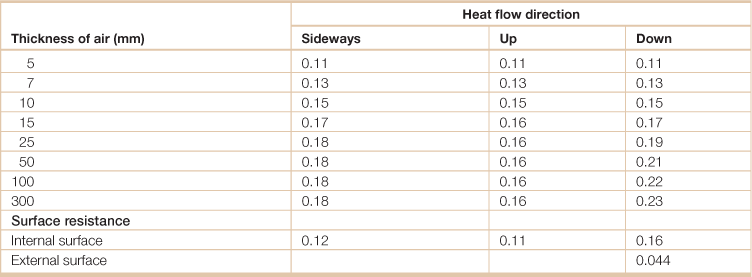
Source: Kalogirou, Soteris A. 2009. Solar Energy Engineering, (Boston, Academic Press).
Table 18.13
Average radiogeneic heat in geological materialsa
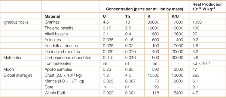
aThe total heat flux per unit mass of the Earth is 7.4 x 10⁻¹² Wkg−1.
Source: Adapted from Stacey, F.D. and P.M. Davis. 2008. Physics of the Earth, 4th ed., (Cambridge University Press, Cambridge, UK).
Table 18.14
Radiative properties of natural surfaces
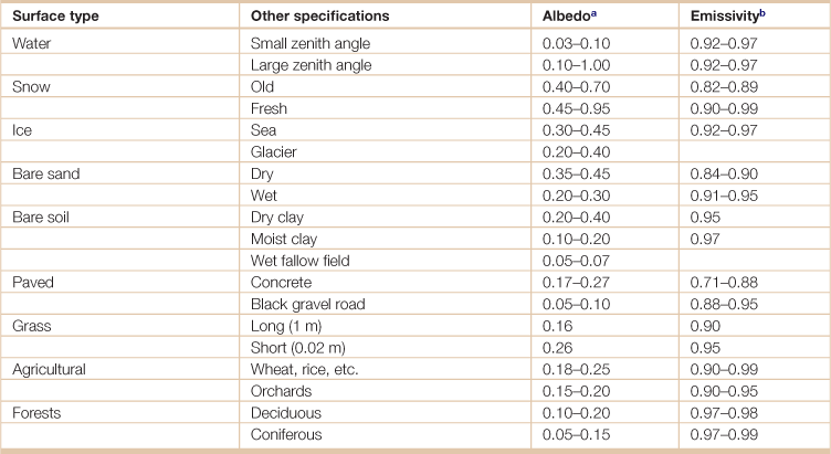
athe ratio of reflected radiation from a surface to incident radiation upon it.
bthe relative ability of its surface to emit energy by radiation, measured by the ratio of energy radiated by a particular material to energy radiated by a black body at the same temperature.
Source: Adapted from Arya, S. Pal. 2001. Introduction to Micrometeorology (Second Edition). (San Diego, Academic Press).
Table 18.15
Infared emissivities (%) of some surfacesa
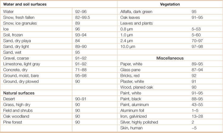
aEmissivity is the relative ability of its surface to emit energy by radiation, measured by the ratio of energy radiated by a particular material to energy radiated by a black body at the same temperature.
Source: Adapted from Hartmann, Dennis L. 1994. Global Physical Climatology, (San Diego, Academic Press).
Table 18.16
Albedos for various surfaces (%)a
| Surface type | Range | Typical value |
| Water | ||
| Deep water: low wind, low altitude | 5–10 | 7 |
| Deep water: high wind, high altitude | 10–20 | 12 |
| Bare surfaces | ||
| Moist dark soil, high humus | 5–15 | 10 |
| Moist gray soil | 10–20 | 15 |
| Dry soil, desert | 20–35 | 30 |
| Wet sand | 20–30 | 25 |
| Dry light sand | 30–40 | 35 |
| Asphalt pavement | 5–10 | 7 |
| Concrete pavement | 15–35 | 20 |
| Vegetation | ||
| Short green vegetation | 10–20 | 17 |
| Dry vegetation | 20–30 | 25 |
| Coniferous forest | 10–15 | 12 |
| Deciduous forest | 15–25 | 17 |
| Snow and ice | ||
| Forest with surface snowcover | 20–35 | 25 |
| Sea ice, no snowcover | 25–40 | 30 |
| Old, melting snow | 35–65 | 50 |
| Dry, cold snow | 60–75 | 70 |
| Fresh, dry snow | 70–90 | 80 |
aAlbedo is the ratio of reflected radiation from a surface to incident radiation upon it.
Source: Adapted from Hartmann, Dennis L. 1994. Global Physical Climatology, (San Diego, Academic Press).
Table 18.17
Top of atmosphere annual mean radiation budget
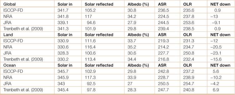
Top of atmosphere annual mean radiation budget quantities for the clouds and the earth’s radiant energy system period of Mar 2000 to May 2004 for global, global land, and global ocean. The downward solar (Solar in), reflected solar (Solar reflected), and net (NET down) radiation are given with the absorbed solar radiation (ASR) and outgoing longwave radiation (OLR)(W m–2), and albedo is given in percent. ISCCP = International Satellite Cloud Climatology Project; NRA = reanalysis of NCAR (National Centers for Atmospheric Research) and NCEP (National Center for Environmental Prediction); JRA = Japanese reanalysis.
Source: Adapted from Trenberth, Kevin E., John T. Fasullo, Jeffrey Kiehl, 2009: Earth’s global energy budget. Bull. Amer. Meteor. Soc., 90, 311–323.
Table 18.18
Direct normal solar irradiance at air mass 1.5a
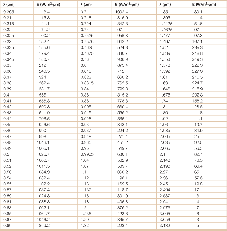
λ = wavelength; E = emissive power.
aDirect normal irradiance is the amount of solar radiation received per unit area by a surface that is always held perpendicular (or normal) to the rays that come in a straight line from the direction of the sun at its current position in the sky. The air mass (AM) coefficient defines the direct optical path length through the Earth’s atmosphere, expressed as a ratio relative to the path length vertically upwards, i.e. at the zenith. “AM1.5” is a common reference in solar energy research and technology.
Source: National Renewable Energy Laboratory.
Table 18.19
Temperature and solar irradiation for select cities in the world
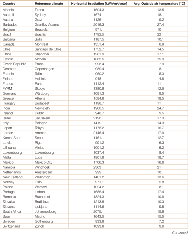
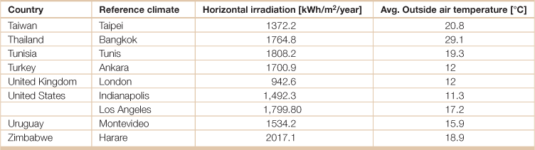
Source: Weiss, Werner and Franz Mauthner. 2012. Solar Heat Worldwide, Markets and Contribution to the Energy Supply 2010, Edition 2012, (Gleisdorf, AEE - Institute for Sustainable Technologies; Paris, Solar Heating and Cooling Programme, International Energy Agency).
Table 18.20
Roughness classificationa
| Surface type | Roughness length (m) |
| Sea, loose sand, and snow | ≈0.0002 |
| Concrete, flat desert, tidal flat | 0.0002–0.0005 |
| Flat snow field | 0.0001–0.0007 |
| Rough ice field | 0.001–0.012 |
| Fallow ground | 0.001–0.004 |
| Short grass and moss | 0.008–0.03 |
| Long grass and heather | 0.02–0.06 |
| Low mature agricultural crops | 0.04–0.09 |
| Low mature crops (“grain”) | 0.12–0.18 |
| Continuous bushland | 0.35–0.45 |
| Mature pine forest | 0.8–1.6 |
| Dense low buildings (“suburb”) | 0.4–0.7 |
| Large town | 0.7–1.5 |
| Tropical forest | 1.7–2.3 |
aThe roughness length is the height above the displacement plane at which the mean wind becomes zero when extrapolating the logarithmic wind-speed profile downward through the surface layer. It is a theoretical height that must be determined from the wind-speed profile, although there has been some success at relating this height to the arrangement, spacing, and physical height of individual roughness elements such as trees or houses.
Source: Adapted from Cataldo, J. and Zeballos, M. 2009. Roughness terrain consideration in a wind interpolation numerical model, Paper presented at 11th Americas Conference on Wind Energy, San Juan, Puerto Rico.
Table 18.21

Source: Adapted from Wizelius, T. 2012. 2.13 - Design and Implementation of a Wind Power Project, In: Ali Sayigh, Editor-in-Chief, Comprehensive Renewable Energy, (Oxford, Elsevier), Pages 391–430.
Table 18.22
Classes of wind power density at 10 meters, 30 meters, and 50 meters elevationa
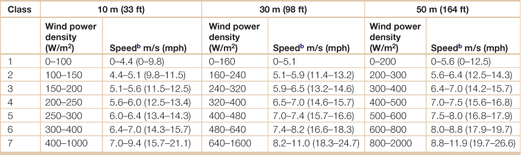
aVertical extrapolation of wind speed based on the 1/7 power law.
bMean wind speed is based on Rayleigh speed distribution of equivalent mean wind power density. Wind speed is for standard sea-level conditions. To maintain the same power density, speed increases 3%/1000 m (5%/5000 ft) elevation.
Source: National Renewable Energy Laboratory.
Table 18.23
Geographic areas of high natural radiation background
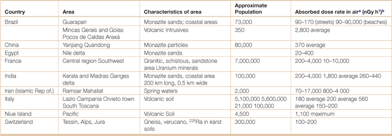
aIncludes cosmic and terrestrial radiation.
bThe Gray (G) is the SI derived unit of absorbed radiation dose of ionizing radiation, and is defined as the absorption of one joule of ionizing radiation by one kilogram of matter (usually human tissue).
Source: United Nations Scientific Committee on the Effects of Atomic Radiation (UNSCEAR), UNSCEAR 2000 Report Vol. 1: Sources and Effects of Ionizing Radiation. United Nations Scientific Committee on the Effects of Atomic Radiation, <http://www.unscear.org/unscear/en/publications/2000_1.html>, Accessed 28 April 2012.
Table 18.24
Radioactive elements in common rocks in the Earth’s crust
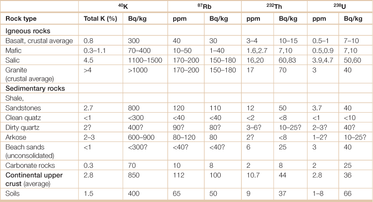
Question marks indicate estimates in the absence of measured values.
The becquerel (symbol Bq) is the SI-derived unit of radioactivity. One Bq is defined as the activity of a quantity of radioactive material in which one nucleus decays per second. The Bq unit is thus equivalent to an inverse second, s−1.
Source: International Atomic Energy Agency. 2003. Extent of environmental contamination by naturally occurring radioactive material (NORM) and technological options for mitigation. Technical Reports Series No. 419.
Table 18.25
Natural radioactivity in the ocean
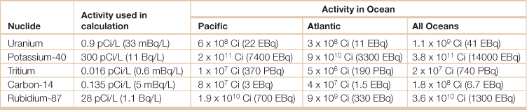
The curie (symbol Ci) is a non-SI unit of radioactivity, and is defined as: 1 Ci = 3.7 × 10¹⁰ decays per second.
The becquerel (symbol Bq) is the SI-derived unit of radioactivity. One Bq is defined as the activity of a quantity of radioactive material in which one nucleus decays per second. The Bq unit is thus equivalent to an inverse second, s−1.
Source: Adapted from The Radiation Information Network, Idaho State University, Radioactivity in Nature, <http://www.physics.isu.edu/radinf/natural.htm>, Accessed 21 November 2009.
Table 18.26
Summary of concentrations of major radionuclides in major rock types and soil

Note: Question marks indicate estimates in the absence of measured values.
Source: International Atomic Energy Agency. 2003. Extent of environmental contamination by naturally occurring radioactive material (NORM) and technological options for mitigation. Technical Report Series no. 419.
Table 18.27
Naturally occurring radionuclides in mineral resources
| Element/mineral | Source | Radioactivity |
| Aluminium | Ore | 250 Bq/(kg U) |
| Bauxitic limestone, soil | 100–400 Bq/(kg Ra) | |
| Bauxitic limestone, soil | 30–130 Bq/(kg Th) | |
| Tailings | 70–100 Bq/(kg Ra) | |
| Copper | Ore | 30–100 000 Bq/(kg U) |
| Ore | 10–110 Bq/(kg Th) | |
| Fluorspar | Mineral | Uranium series |
| Tailings | 4000 Bq/(kg Ra) | |
| Iron | Uranium series | |
| Thorium series | ||
| Molybdenum | Tailings | Uranium series |
| Monazite | Sands | 6000–20 000 Bq/(kg U) |
| Thorium Series (4% by weight) | ||
| Natural gas | Gas, average for groups of US and Canadian wells | 2–17 000 Bq/(m3 Rn) |
| Gas, average for groups of US and Canadian wells | 0.4–54 000 Bq/(m3 Rn) | |
| Scale, residue in pumps, vessels and residual gas pipelines | 100–50 000 Bq/(kg210Pb/210Po) | |
| Oil | Brines or produced water | Ranging from mBq to 100 Bq/(L Ra) |
| Sludges (scales) | Ranging up to 70 000 Bq/(kg Ra) Typically 103–104 Bq/kg, ranging up to 4 × 10⁶ Bq/(kg Ra) | |
| Phosphate | Ore | 100–4000 Bq/(kg Unatural) |
| Ore | 15–150 Bq/(kg Thnatural) | |
| Ore | 600–3000 Bq/(kg Ra) | |
| Potash | Thorium series 40K | |
| Rare earths | Uranium series | |
| Thorium series | ||
| Tantalum/niobium | Uranium series | |
| Thorium series | ||
| Tin | Ore and slag | 1000–2000 Bq/(kg Ra) |
| Titanium (rutile, ilmenite) | Ore | 30–750 Bq/(kg U) |
| Ore | 35–750 Bq/(kg Th) | |
| Uranium | Ore | 15 000 Bq/(kg Ra) |
| Slimes | 105 Bq/(kg Ra) | |
| Tailings | 10 000–20 000 Bq/(kg Ra) | |
| Vanadium | Uranium Series | |
| Zinc | Uranium Series, Thorium Series | |
| Zirconium | Sands | 4000 Bq/(kg U) |
| Sands | 600 Bq/(kg Th) | |
| 4000–7000 Bq/(g Ra) |
The becquerel (symbol Bq) is the SI-derived unit of radioactivity. One Bq is defined as the activity of a quantity of radioactive material in which one nucleus decays per second. The Bq unit is thus equivalent to an inverse second, s−1.
Source: International Atomic Energy Agency. 2003. Extent of environmental contamination by naturally occurring radioactive material (NORM) and technological options for mitigation. Technical Reports Series No. 419.
Table 18.28
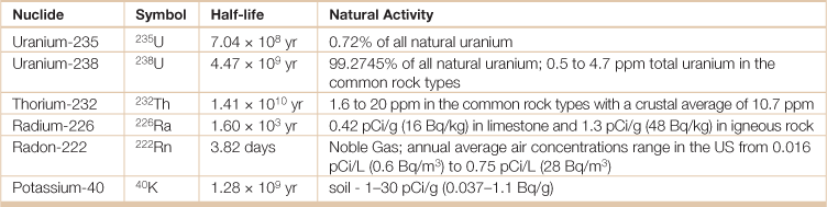
Primordial radionuclides are those left over from when the world and the universe were created, and which have not completely decayed due to their long half-life. They are typically long lived, with half-lives often on the order of hundreds of millions of years. Primordial radionuclides also include those generated from the primordial radionuclides U-238, U-235 and Th-232 of the associated decay chain. The becquerel (symbol Bq) is the SI-derived unit of radioactivity. One Bq is defined as the activity of a quantity of radioactive material in which one nucleus decays per second. The Bq unit is thus equivalent to an inverse second, s−1. The curie (symbol Ci) is a non-SI unit of radioactivity defined as 1 Ci = 3.7 × 10¹⁰ decays per second.
Source: Adapted from the Radiation Information Network, Idaho State University, Radioactivity in Nature, <http://www.physics.isu.edu/radinf/natural.htm>.
Table 18.29
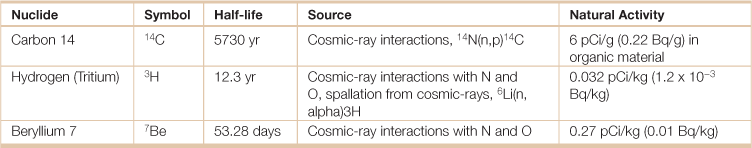
Cosmic radiation originates directly or indirectly from extraterrestrial sources. The radiation is in many forms, from high speed heavy particles to high energy photons and muons. The upper atmosphere interacts with many of the cosmic radiations, and produces radioactive nuclides. Some have long half-lives, but the majority have shorter half-lives than the primordial nuclides. Some other cosmogenic radionuclides are 10Be, 26Al, 36Cl, 80Kr, 14C, 32Si, 39Ar, 22Na, 35S, 37Ar, 33P, 32P, 38Mg, 24Na, 38S, 31Si, 18F, 39Cl, 38Cl, 34mCl.
Source: Adapted from The Radiation Information Network, Idaho State University, Radioactivity in Nature, <http://www.physics.isu.edu/radinf/natural.htm>.