
Performance Prediction
Abstract
This chapter covers the key field of performance prediction: calculating static, dynamic, and thermo-fluid performance for design elements. Starting with simple materials performance, including stress, bending, and fatigue analysis, it continues with FEA, using some real-life examples, and reiterates the need for verification of calculated results to avoid computer-aided failure.
6.1 Why Performance Prediction is Necessary
When a product is designed and built, the designer needs to specify what the product is capable of achieving and how it may perform. Without performance prediction techniques, the specification of performance would be guesswork. Some designers might estimate materials and strengths by sheer experience. This is a dangerous game, as it could result in a structure that is too weak or one that is heavily overdesigned. Traditionally, designers have made structures heavier than necessary to be “on the safe side.”
To optimize material usage and potentially drive down the cost of products, product performance prediction needs to be as accurate as possible within specified limits. A Formula One racing car engine is designed for high performance but to last for only one race, after which it is refurbished and any sacrificial or worn components replaced. This level of accurate performance prediction can only be achieved using sophisticated mathematical techniques in various fields, the most common of which are listed as follows:
• Stress analysis
• Vibration analysis (dynamics)
• Mechanical analysis (velocity motion, inertia, energy, power, etc.)
• Fluid dynamics analysis
• Thermodynamic analysis
Performance prediction can generally be split into two categories:
• Performance prediction to ensure the product is safe
• Performance prediction to obtain a precise working specification
Engineering analysis combines a fundamental understanding of natural phenomena, the laws of physics, and a mathematical ability with which the designer can arm himself in order to perform a particular analysis for a particular product for a particular situation.
6.2 Historical Aspects of Analysis
Modern man has always manufactured tools as aids to living. Early Homo sapiens designed hunting tools such as spears and clubs. If the tools did not work or broke during use, they were modified until they worked, creating a trial and error approach to design. As time went on, society required more sophisticated products such as carts, bridges, advanced weaponry, and so on. Up to the late Middle Ages, the devices so built were not designed in the modern sense but were manufactured and tried out. If the devices did not work, they were modified.
During the Industrial Revolution, engineers began to quantify some of the parameters that would assist in the design of various devices and products, but still, much of the work was based on experience. Many engineers gained their “experience” from one or more failures: learning from their mistakes. Famous engineers such as Brunel, Telford, Arkwright, and Stephenson were gifted people who were able to quantify some of the parameters of their designs and who had a wealth of experience to guide them on the remainder.
Modern design began to emerge when drawings and plans were created so that builders, engineers, and other artisans could understand what was in the mind of the lead engineer. True design came of age when science and mathematics were applied to the design of structures and other artifacts. Engineers and mathematicians such as Newton, Bernoulli, Reynolds, Euler, Boyle, and Faraday, among many others, experimented in the physics of their field to define laws and to apply the mathematics to model physical phenomena. This assisted later engineers, who applied these mathematical principles on future projects and individual designs.
Perhaps the greatest and earliest breakthrough of modern engineering mathematics was by a Ukrainian Stephen P. Tymoshenko (1878-1972), who is known as the father of modern engineering mechanics.
Tymoshenko was instrumental in developing “the theory of elasticity,” which quantifies and sets out analytical techniques for calculating stresses and strains in materials under varying loads. He expanded his theorems and techniques to include general mechanics and buckling plus many other areas of stress analysis, which engineers now use as an everyday tool in their analytical armory. It is significant that Tymoshenko also used the Rayleigh method of Finite Element Analysis as early as 1911. After moving to the United States in 1922, Tymoshenko became a professor, first at the University of Michigan and later at Stanford University where he and his research teams greatly expanded stress analytical techniques and methods.
With the advent of quantifiable stress analysis techniques, it was possible to analyze components using computing power. The finite element method of stress analysis had been known for decades, but its use only became widespread with the development of more powerful and sophisticated computers.
6.3 Materials Testing
The analytical techniques put forward by Tymoshenko and others were excellent tools for predicting the stresses within a component, but these calculated stresses had to be weighed against the strength of the material. Alongside the expansion of analytical techniques was an expansion in testing methods, which quantified the strength of the material plus many other parameters.
Materials such as steel behave in different ways under different conditions. Perhaps the most useful test is the tensile test where a standard-sized specimen is put into tension (pulled apart) until it breaks. The result of such a test provides information about the following:
• elasticity (Hook’s Law)
• yield point of the material
• toughness (energy of mechanical deformation prior to rupture)
• ultimate tensile strength (UTS)
A typical graphical plot of stress against strain (force against extension will give the same results) is shown in Figure 6.1.
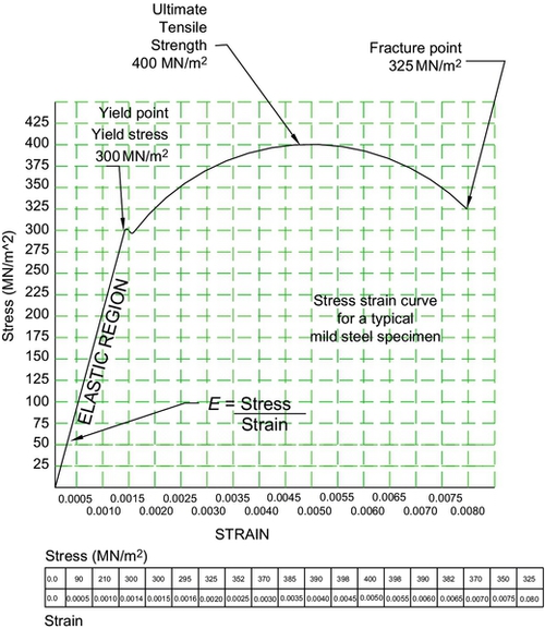
Figure 6.1Typical Tensile Test Characteristic for Mild Steel [1].
6.3.1 Elastic region
Any material possesses elasticity when stretched and behaves according to Hook’s Law. When the material is stretched within the elastic region, upon release, it will spring back to its original position without being permanently deformed.
6.3.2 Yield point
A material that is stretched up to its yield point will always spring back to its original position when released. If the yield point is passed, then the material is said to be in a “plastic” state and will remain deformed.
6.3.3 Ultimate Tensile Strength (UTS)
This is the maximum strength of the material and is often used as a comparison to theoretically calculated stresses.
6.3.4 Fracture point
As the tensile specimen is stretched, it will break at the fracture point.
6.3.5 Young's Modulus E
This is sometimes called the “Elastic Modulus.” It can be calculated as follows:

The elastic modulus when calculated thus has units of GN/m2. Depending on the toughness of the material, the slope of the characteristic within the elastic region will change. If the characteristic is very steep, the material can be considered to be tough. This is the case with steel, where a high stress (or force per unit cross-section) applied to a specimen will give only a small strain (extension). On the other hand, if the angle is very low such as that recorded by stretching an elastic band, a small stress would lead to a very large strain. Clearly, the elastic band is not as tough as a steel specimen.
These and many other valuable parameters that describe the specification of the material allow a comparison of calculated stress against the strength of the material.
Example: Actual Stress Compared with Material Strength
A ϕ 10 mm mild steel tie rod has to be placed in tension in a roof structure and has been shown to be under a load of 10 kN. Using basic stress analysis, the calculated stress σ in the material can be seen as follows:

where d is the diameter of the mild steel bar.
Basic tensile tests on mild steel specimens have shown that the ultimate tensile strength (UTS) is 320 MN/m2, the value of which can be compared against the theoretical stress in the tie rod. In this case, the theoretical stress is much less than the actual strength of 320 MN/m2, rendering the tensile rod safe in this application.
Confidence in analytical “predicted” stresses and, further, confidence in the strength of the materials data derived from laboratory tests provides engineers with the tools to show that a component or product is safe under an assumed loading regime.
There are many forms of data that may be provided for a particular material. The tensile test mentioned earlier is one of the most useful of them, but there are others such as torsion tests, fatigue tests, impact tests and many, many more.
For instance, the resistance to a shock load depends on how the energy is absorbed by the material. A material such as steel can be in its natural, malleable state or in a hardened state, so shock loading will have different effects. If, for instance, a mild steel bar is placed in a vice and hit with a hammer, the bar will absorb much of the energy and merely bend. If the same treatment is applied to a bench file, which is hardened and very brittle, the file will shatter. A small amount of energy will have been absorbed but the material cannot absorb much energy because of its brittleness.
The test developed for this application is the “Izod” or “Charpy” test and measures the energy absorption by the material under a prescribed shock load. A diagram of a typical test operation can be seen in Figure 6.2.
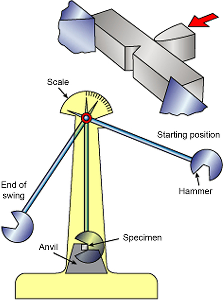
Figure 6.2Typical Izod/Charpy Test [2].
Standard information for particular materials is available from many diverse sources such as from textbooks, data files, and, of course, the Internet. It is incumbent on the designer to build a data file as he/she progresses through his/her career.
6.4 Factor of Safety
Once we have the means to calculate theoretical stresses and the ability to compare those results against test data for the material, the inevitable question that arises is “how many times safer a structure is when placed under anticipated loads.” Before finding the answer to this question, another question needs to be answered: “Why would a device need to be several times safer than suggested by the anticipated loading?”
Though stress analysis can give the engineer anticipated working stresses within the material and the structure, inaccuracies are inevitable. Generally, it can be assumed that any calculated stresses are only 80% accurate. Furthermore, there are uncertainties in the structural regime which include the following:
• Material integrity (inclusions, blowholes, inaccurate welds, etc.)
• Inaccurate calculations
• Overloading (abuse by the user)
• Aggressive environment (weaknesses caused by early corrosion)
• Consequences of failure (failure of the structure could lead to fatalities)
• Cycling loading leading to a weakened structure
• Change in material microscopic structure as a result of fastening techniques such as welding
A system of factors of safety can be applied to a structure, which will allow for the uncertainties listed here. These general factors of safety are shown in Figure 6.3, but it should be noted that more specialized and detailed safety factors may be employed by professionals working in individual industries.
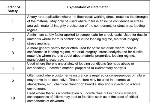
Figure 6.3General Factors of Safety [1].
6.5 Consolidation of Safety in Structures and Devices
The ability to accurately analyze and define the stresses within a structure combined with the ability to derive accurate material strengths from experimental data has inevitably led to the quantifying of structural safety. The use of factors of safety now allows engineers to create a specific safety margin. If, for instance, a structure possesses a factor of safety of 4, it can be said with confidence that the structure is four times safer than the envisaged loading regime.
The three factors, therefore, that allow engineers to predict structural safety are as follows:
1. Accurate predictive stress analysis
2. Accurate structural data derived experimentally
3. Application of factors of safety
Example: Factor of Safety Applied to a Bridge Structure
A footbridge was to be designed with an overall safety factor of 4, which was intended to be applied to any component within the bridge structure. This was to cover for overloading, errors in manufacture, use in the natural environment (wind forces, corrosion, etc.) and gentle cycling loading. The material’s ultimate tensile strength was found to be 400 MN/m2 from lookup tables for the material. The safety factor was applied as follows:


When calculating working stresses, the designers must therefore apply materials to the bridge structure whose working stresses do not exceed 100 MN/m2.
Example: Multiple Safety Factor
A cargo crane was to be designed to be fitted to an oil rig supply ship for duty in the North Sea. The designers realized that it would be necessary to apply multiple safety factors to cope for various conditions such as those listed here:
• uncertainties with regard to material integrity
• low-temperature brittleness (reducing the ductility of the material)
• corrosive environment
• shock loads
• abusive use (overloading)
• cycling loading
It was decided to apply factors of safety as follows:
5 To cover shock loads
abuse
uncertainties regarding material integrity
abusive use
2 To cover a corrosive environment
2 To cover cycling loading
2 To cover low-temperature brittleness
When these safety factors are combined, the overall safety factor becomes 11.
Example: Pivot Points on the “Car Stacker”
It is sometimes necessary to overdesign components so that they “look right” and the user is reassured that the components possess appropriate strengths. This involves applying a much greater factor of safety than would normally be necessary.
The Car Stacker 3D parking system shown in Plate 6.1 accepts a car on the ramp, which then slides forward to allow a second car to be parked underneath. The pivot, cantilever shafts were calculated at 20 mm diameter, which included an adequate safety factor. However, it was considered that they might not appear to be very strong and that users might not feel confident about parking their expensive cars underneath the ramp when it was loaded with another vehicle. In this case, the consensus was that it would be better to increase the diameter of the pivot pins to 50 mm, thus overdesigning the pivot pin by giving it a safety factor of 15. The ultimate aim was to ensure that the pin was safe, but primarily it was to make it “look” safe and give confidence to the user.

6.6 Computing Power
The radical improvement in computing power over the last 30 years has powered the development of software that can not only compute stresses but through the finite element method develop a 3D picture of stresses throughout a structure or component. Finite element methods have also been applied to branches of engineering other than stress analysis. Areas such as thermal analysis, fluid dynamics analysis, and vibrations analysis have all benefited from these methods.
The use of specifically designed software has also reformed the way in which engineers consider a problem. If an engineer was designing a beam, for instance, he would consider the loading regime, calculate the point of highest stress, and design the beam to cope with that stress. The engineer would apply a reasonably high factor of safety, which would enlarge the beam. Use of more sophisticated calculation and modeling software could allow the beam to be honed and tuned to fit the loading regime.
When designing a beam, the strength is dependent on the shape of the beam section; a larger beam section generally means more mass. If the greatest stress is at the center of a simply supported beam, then the section has to be largest at that point. This also means that the section can be reduced toward the ends of the beam because there are lower bending stresses experienced at these points. Although standard beam calculations can be used to calculate the section along the length of the beam, computing analysis can greatly speed up the process.
A typical structure that has been designed to these parameters is shown in Plate 6.2.
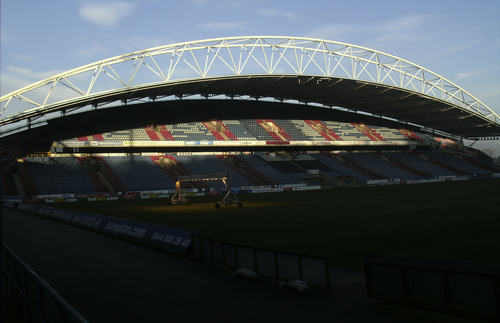
Plate 6.2Stadium Roof [3].
It can be seen in Plate 6.2 that the beam supporting the roof of the stadium is simply supported, that is, the support points are at each end of the beam. The greatest stress is in the center of the beam at which position is the deepest beam section. Stresses are applied to the beam toward the support points but they are much lower than at the center. It means that the beam section toward the support points does not have to be as large as at the center. This is typical of the tuning that computing power allows engineers to achieve.
6.6.1 Design iteration supported by computer-aided analysis
The use of computer-aided analysis has become an almost indispensable tool. There is often a compromise between the strength and weight of a component or structure. The use of computer-aided analysis is an important factor in reducing the weight while retaining the strength.
Example: The Design of a Foot Pedal Arrangement for a Lightweight Sports Car
A foot pedal arrangement for a lightweight car has to not only possess strength for arduous use, but it also needs to be as light as possible. The design iteration of such a foot pedal box is shown later.
The final concept design for a foot pedal arrangement for a high-performance lightweight vehicle can be seen in Figure 6.4.
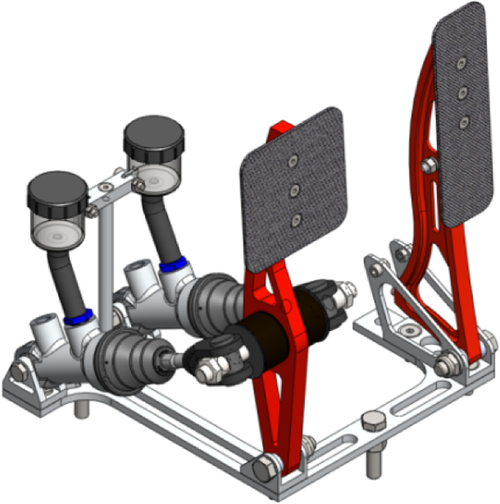
Figure 6.4Final Concept Design for a High-Performance Vehicle [4].
During the deign process, it emerged that the need for weight reduction while maintaining performance had become key to the design.
The following figures give a step-by-step illustration of the design process using computational stress analysis techniques to drive the iterative process of design optimization within two apparently conflicting parameters (Figure 6.5).
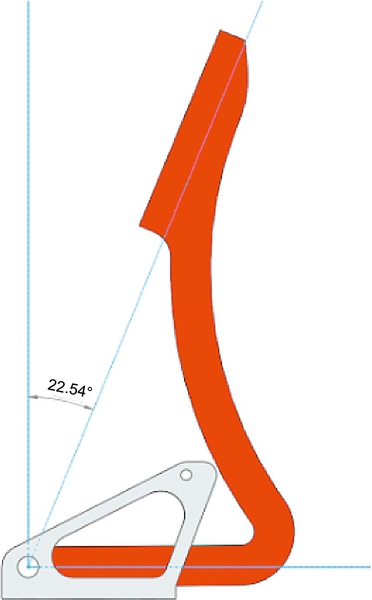
Figure 6.5Side View of the Accelerator Pedal Initial Concept Design [4].
Computational stress analysis revealed that this shape was low in weight but did not possess the strength required. Figure 6.6 shows where the accelerator pedal would fit in the pedal box design. The next iteration was to start from a solid plate and gradually remove material. The first solid plate iteration can be seen in Figure 6.7.
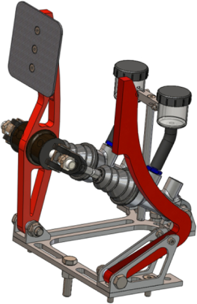
Figure 6.6Initial Concept Design of the Accelerator Pedal Shown In Situ in the Pedal Bracket [4].

Figure 6.7First Solid Plate Iteration Without Weight Saving [4].
Removing material from the solid plate model using 3D computer modeling, and applying finite element analysis allowed weight reduction while retaining strength in critical areas. After several further iterations, the analytically stressed model that can be seen in Figure 6.8 was built.
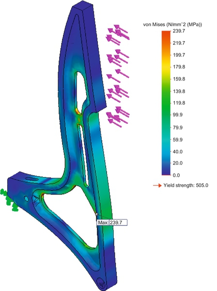
Figure 6.8Finite Element Stress Analysis Model of Concept 2 [4].
6.7 Fatigue Strength Prediction
One of the most critical performance predictions is predicting fatigue strength. As a rule of thumb, it can be considered that if something moves, it will be subjected to cycling loading. An applied load that cycles backward and forward may not initially overcome the strength of the material but constant cycling loading may eventually form a fatigue crack leading to complete failure.
Take a disused credit card and bend it backward and forward. A crease line will appear and the plastic will tend to turn white. On close inspection, the plastic looks crystalline along the crack. Eventually the card will break along the bend line. This is essentially a fatigue break. The phenomenon is well known to engineers who ignore the occurrence at their peril. There are many examples.
Example: The Comet: The First Jet Airliner
The de Havilland DH 106 Comet was the first commercial jet airliner to reach production and ushered in the jet age of air passenger travel. It featured an aerodynamically clean design with four turbojet engines buried in the wings, a pressurized fuselage, and large square windows. Just a year after entering commercial service, the Comets began suffering problems, with three of them breaking up in mid-flight.
The pressurized cabin was a relatively new development. During a normal flight, when the aircraft climbed to its normal cruising height, the cabin was pressurized to around 11 psi, the ambient pressure outside the cabin being much less than this. The difference in pressures meant that the fuselage was like a balloon with pressure on the inside stretching the aircraft skin. When the aircraft landed and the cabin depressurized, the stresses in the fuselage were relaxed. This was a classic case of cycling loading.
The Comet was withdrawn from service and extensively tested to discover the cause. Investigations found that the problem was catastrophic metal fatigue, which was not well understood at the time. Design flaws were ultimately identified, including square windows, which created “stress raisers” in the corners of the windows. These allowed fatigue cracks to propagate. The Comet was extensively redesigned with oval windows and structural reinforcement.
6.7.1 Welded joints
If a welder is asked to define the strength of his weld, he will say that it is as strong as the parent metal. The fact is that under cyclic loading, the weld will break because of the changing metallic structure around the welded joint. This was the problem with the Liberty ships in World War II, which sank not due to enemy action, but due to welded joint failure under the cyclical load imposed by the waves. Fatigue cracks propagated within the brittle weld boundaries leading to a catastrophic failure of the ships’ hulls. The problem was solved by transforming the metallic structure by annealing so that the welded joint metallic structure became malleable as was the parent metal.
If a welded specimen is placed in a vice and struck with a hammer, the specimen will bend. If it is repeatedly bent backward and forward, it will tend to break along the welded joint. The metallic structure can be transformed back to the original malleable metallic structure by annealing. This is a process in which the material is heated to “a cherry red color” and allowed to cool naturally.
Some structures are too large to anneal unless specialist tooling is used. Often, designers create a welded structure allowing for weld brittleness by increasing the size of the weld. In critical cases where cyclic loading may be a problem, welded joints should be avoided unless there is a secondary retaining system such as bolts.
6.7.2 Quantifying fatigue life
Fatigue prediction is notoriously difficult. Two components manufactured in the same batch and subjected to the same cyclic loading conditions are unlikely to break from fatigue at exactly the same time. Some of the minutest variations may change the way the component behaves. Typically, variations might include loading regime, difference in size (perhaps the difference in a high or low tolerance), material uniformity, and differences in surface finish. Perhaps the two most significant variations between components are in the surface finish and the material integrity.
Welds are usually applied manually, and so can suffer slight variations in heat input, blowholes, uniformity, etc.
Materials, though appearing to be the same, may have dense spots, or metallic inclusions, or blowholes when cast. These differences will serve to change the performance at a microscopic level and will inevitably have an effect on the fatigue life of the component.
Perhaps the most significant effect on fatigue life is that of surface finish. When viewed at a microscopic level, surface finish appears as a series of peaks and valleys, where the bottoms of the valleys are often very sharp. Figure 6.9 shows a typical 3D surface finish profile. The reading was measured on a Talysurf PGI-contacting stylus profilometer (Ametek Taylor Hobson) with an average roughness of 15 μm. The same roughness profile can be seen as a 2D profile in Figure 6.10.
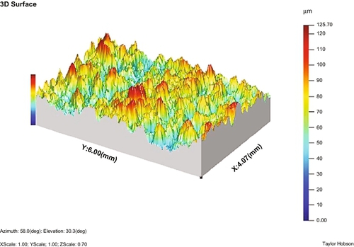
Figure 6.9A Typical 3D Surface Finish Profile with an Average Roughness of 15 μm [5].
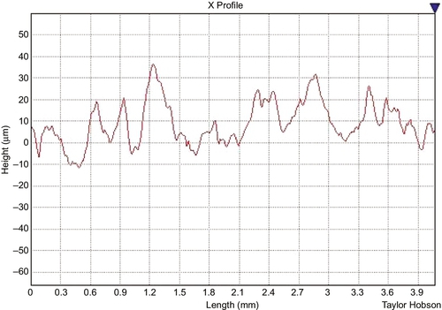
Figure 6.10The Surface Profile of Figure 6.9 Shown as a 2D Surface Finish Profile with Average Roughness of 15 μm [5].
The reader should note that the sample area is 6 mm × 4 mm, but the height of the peaks has been exaggerated to enhance visibility. The rough nature of the surface is fairly typical of surfaces when viewed at a microscopic level. It is clear to see that the acutely sharp nature of the base of the valleys may easily make this area the start of a fatigue crack should cycling loads be applied to that area.
It is often useful, for instance, for measurement purposes, to take a slice through the 3D profile to reveal a 2D profile, as shown in Figure 6.10.
If stresses are applied to, say, a shaft, a crack may propagate from one of these valleys. In fact, any sharp corner, scratch, or interruption (stress raiser) in the smooth surface finish may become the beginning of the propagation of a crack. Fatigue cracks always start at stress raisers, so removing such defects increases the fatigue life.
A smooth finish is, therefore, very important if it is known that a component will be cyclically loaded. In gear manufacture, when each gear tooth rotates and meshes with the opposite gear tooth, it is cyclically loaded for just a few milliseconds before being released from contact. During the next cycle, the tooth makes contact once again. Gear teeth, therefore, can suffer severe cycling loading. Understanding this phenomenon, precision gear manufacturers manufacture the gear teeth to a very smooth surface finish, thus extending the life of the gear teeth (Plate 6.3).
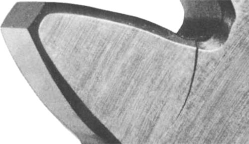
Plate 6.3Gear Tooth Crack Propagation [6].
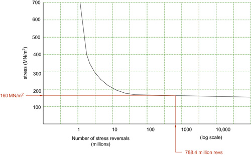
6.7.3 S-N Curves (Goodman Curves)
It is well known that the bending of a piece of material backward and forward eventually leads to the breaking of the material. The breaking of the credit card is just such an example. A great deal of work has been done in this field to determine the number of cycles that materials may suffer before breaking. The diagram in Figure 6.11 shows generic S-N curves (stressed/number of cyclic reversals); sometimes these graphs are called Goodman curves after the engineer who accomplished much work in the area of fatigue.
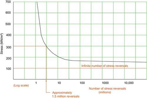
Figure 6.11Idealized S-N Curve (Goodman Curve) [1].
The graph line in Figure 6.11 plots applied stress on the vertical axis and the number of stress reversals on the horizontal axis. If the applied stress on a component is, say, 300 MN/m2, the number of stress reversals before failure would be in the region of 1.5 million.
If now the material section is modified so that the applied stress becomes 100 MN/m2, it can be seen that the material can cope with an infinite number of stress reversals because the S-N curve indicates that stresses at that level will never become dangerous.
The graph shown in Figure 6.11 is an idealized curve. Normally these curves are produced from empirical data for specific materials in different states. For instance, EN 8 (080M46) will have different S-N curves for its natural state compared to its hardened state. These curves can normally be obtained from materials suppliers.
Example: Shaft with Cycling Loading
A shaft protrudes from Bearings 150 mm to the center of a chain drive sprocket.
Consider a notional stressed element of the shaft shown in Figure 6.12. The load applies a tensile stress to the outer layer of the shaft at the element, but as the shaft rotates through 180°, the same part of the shaft under the element sees a compressive stress. As the shaft rotates back to its original position, the element sees a tensile stress once again. Through every revolution of the shaft, this “stress reversal” continues to happen. It is the same condition that the credit card experiences when it is bent backward and forward until it breaks (Figure 6.13).
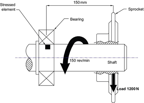
Figure 6.12Cantilever at Shaft Showing Stressed Element [1].
Shaft parameters
150 rev/min
Factor of safety (FoS) of 3
Shaft material: medium carbon steel σUTS = 600 MN/m2
Calculate the shaft diameter when a static load is applied
Find the working stress σw![]()
or![]()
Find the maximum bending moment
Mo = Load × moment arm = 1200 × 0.15 = 180 Nm
Find the shaft diameter
From![]()
![]()
![]()
d = 0.0209 m or 21 mm
The shaft diameter has been calculated at ϕ 21 mm assuming a static load with a factor of safety of 3. This would normally be assumed to be safe, but in this case cycling loading is applied with the incumbent stress reversals.
Determine the shaft diameter taking into consideration the requirement for an almost infinite number of stress reversals
Application parameters
Continuous operation for 10 years
150 rev/min
Shaft material: medium carbon steel σUTS = 600 MN/m2
Determine a number of stress reversals (N) within the expected life
N = 150 rev/min × 60 min × 24 h × 365 days × 10 years = 788.4 million rev
Apply the expected number of stress reversals, 788.4 million, to the diagram in Figure 6.12. It can be seen that the maximum stress to which the shaft can be submitted is 160 MN/m2. To determine some safety margin and to extend the life of the shaft, it is proposed to make the maximum working stress 100 MN/m2.
Determine the shaft diameter using a working stress σw of 100 MN/m2
Previously calculated bending moment = 180 Nm
From![]()
![]()
![]()
d = 0.0264 m or 27 mm
The result of the consideration of stress reversals is to increase the diameter of the shaft, which reduces the applied stress and thus increases the number of stress reversals to which the shaft can be subjected.
6.7.4 Stress Concentrations
The “S-N” curve described earlier is an excellent method of predicting the life of a component in which there are stress reversals; however, it is important to realize that fatigue cracks usually start from an abrupt change in the surface condition of the material such as small holes, screw threads, scratches, machine tool striations, and many other surface defects. It is incumbent on the design engineer to understand the stresses applied at the surface of a component and to eliminate stress concentrations at the most highly stressed positions on the surface.
There are, however, discontinuities on the surface of the component, which are necessary, perhaps to house other components such as bearings or gears. These elements could be shoulders or undercuts that effectively leave sharp corners from the machining process. An example could be the 90° corner left at the bottom of a keyway or perhaps a shoulder turned onto a shaft. These “designed-in” surface discontinuities can be built in to the stress calculations for the shaft.
Example: A spur gear is held in an axial position along the shaft by a spacer on one side of the gear and on the other side by a shoulder machined onto the shaft. In any machining operation, the tool tip radius would leave a very small radius at the base of the shoulder, shown in Figure 6.14, preventing the spur gear from properly contacting the shoulder. A relief groove may therefore be applied such as that shown in Figure 6.15. Since this is effectively a stress concentration, which is designed into the shaft, it may be included in the stress calculations for the shaft using data from Peterson [7]. Please also see Figure A6.3, also in Appendix.
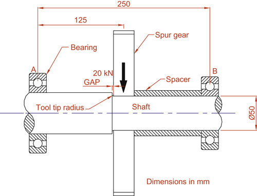
Figure 6.14Spur Gear Mounted on a Shaft Between Two Bearings [1].
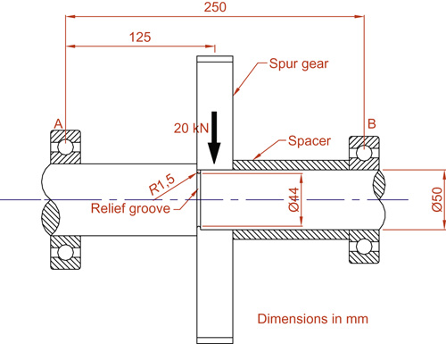
Figure 6.15Spur Gear Mounted on a Shaft Showing Relief Groove [1].
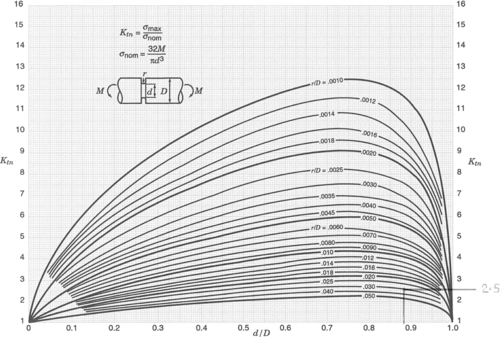
Figure A6.3Stress Concentration Factors for Shaft with Relief Groove [7].
Stress analysis. In order to compare the shaft with and without the relief groove, there are two sets of calculations to be performed. These calculations can be seen in Appendix A6.1 with a synopsis indicated below:
(1) Maximum allowable stress for the shaft shown in Figure 6.14 = 101.9 MN/m2
(2) Maximum allowable stress for the shaft shown in Figure 6.15 = 11.5 MN/m2
The value of σmax = 11.5 MN/m2 can be considered to be the maximum stress the shaft can undergo when such a relief groove is applied to the shaft. Consider the maximum stress the shaft can undergo when there is no relief groove. The value of 101.9 MN/m2 is a factor of 10 greater than the maximum stress in the shaft with a relief groove. The reduction in strength is a consequence of designing into the shaft a legitimate stress raiser, but it should be considered that the analysis has allowed a precise design to be created that caters to a reduction in strength.
6.8 Performance Prediction Methodology and Application
In the early pages of this chapter, it was stated that there are generally two reasons for performance prediction
• Performance prediction to ensure the product operates within safe limits
• Performance prediction to obtain a precise working specification
Examples have thus far centered on stress analysis, which is normally used to ensure that structures or devices possess the strength to cope with the applied loads. A great deal of analysis, however, is carried out to predict how a product might behave and to enable the correct selection of components that may be purchased from an outside source.
Behavioral analysis might be used, for instance, to calculate the parameters of a bought-out product such as a vibration isolator. An example can be seen in Appendix A6.6. This example outlines a manual method of selecting an appropriate spring stiffness, which can then be used to select an isolator from a catalog. Vibration isolation vendors often offer an online selection process where the purchaser can enter appropriate parameters into the software. This will then calculate and automatically select a suitable isolator.
Many component vendors such as bearings and seals suppliers offer similar on-line services. Since the design information is the key to efficient design creation, the ease of selection of components not only assists the designer but also ensures that the designer will continue to go back to the particular supplier who offers the most easy-to-access information.
Behavioral analysis may also be used to predict the product’s performance when performance targets have been set perhaps by the marketing team or perhaps within the Product Design Specification (PDS). The example outlined in Appendix A6.3 describes the analysis of a torsion meter attached to a ship's propeller shaft. The eventual outcome is predicting the total angular deflection, 9.83° along the whole 13 m length of the propeller shaft.
Appendix A6.4 describes the dynamics of powering a bicycle and, under certain circumstances, predicts the forces at the brake blocks, the driving forces at the road-tire interface, the work done by the rider, and the power requirement.
Appendix A6.5 describes the power requirement for lifting a mass via a winding drum. This kind of analysis can be used to select the power plant such as the diesel engine.
Performance prediction analysis can also be used to assist the build process and help to prescribe the method of use of the product. Predictive analysis was successfully used in the case of the Denby Dale pie challenge. Denby Dale is a village in West Yorkshire renowned as the village that creates the largest meat and potato pies in the world. The last attempt was the Millennium Pie challenge in 2000, which was to cook 12 tons of pie filling and distribute it to 40,000 people on “pie day.” See Plate 6.4. The author, along with his close colleagues, was set the task of designing the “pie cooker.” The cooker dimensions were 12 m × 2.3 m × 1 m and it housed 24 vats, each holding 500 kg of pie filling and each being heated by individual elements.
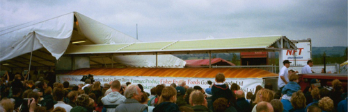
Plate 6.4The Denby Dale Pie Transported by the Low Loader Emerging from the Cooking Tent [1].
One of the criteria was that the whole pie should be paraded around the village before it was returned to the serving field where the contents would be distributed to the audience. Initial estimates put the contents at 12 tons and the cooker structure at 6 tons resulting in a total mass of 18 tons. This clearly required a low loader truck systems for the transportation through the village and back to the “pie field.” In fact, the cooker dimensions were determined by the size of the low loader transporter.
The cooker was designed as a beam with the normal standard beam analysis, which can be seen in Appendix A6.7. This is clearly an example of analysis that has been performed on a structure so that it can be used safely.
It was essential that ingredients were added to the pie filling in a precise fashion so that temperatures did not fall below 65 °C, which would trigger the growth of the Clostridium perfringens bacterium. This is the bacterium that causes food poisoning and typically causes victims to develop diarrhea and sickness. The cooking process involved heating the ingredients of each VAT to 100 °C and then adding further ingredients such as chopped potatoes, onions, seasoning, etc. It was the task of the designer to calculate, using the principles of heat transfer, the mass of ingredients which could be added before the pie filling temperature was reduced to 65 °C. This analysis can be seen in Appendix A6.8 and was performed primarily for safety reasons and also to define the methods by which ingredients were added to the mix of the pie filling.
6.8.1 Computational analysis overview
Before the advent of computer aids, analysis was achieved largely using manual calculations. These calculations were not only tedious but also very limiting in that they could not allow analytical sophistication beyond the use of a good calculator. Furthermore, assumptions made during the calculation process often reduced the accuracy of the analytical model. Safety factors were, therefore, increased to compensate for these inaccuracies.
Modern analytical software often eliminates the need for these rule-of-thumb safety factors, allowing more efficient use of materials and better performance prediction.
6.8.2 Basic electronic calculation tools
The advent of scientific calculators provided engineers with a very powerful calculation tool, which was more accurate and more convenient than the previous and very common slide rule. Calculation tools became more and more powerful with the advent of personal computers and the complementary software. Spread sheet packages allowed engineers to create lengthy and repetitive analysis, thus avoiding writing specific programs in languages such as Fortran or C++. Though these languages are useful and may still be relevant to the engineer’s armory, it is often much more convenient to use spreadsheet packages in which engineers can input equations and link cells to other cells.
6.8.3 Advanced computational analytical techniques
Advanced computational analysis relies on the theory of the finite element and originated from the need to solve complex elasticity and structural analysis problems. The origin of the finite element can be traced back to work originally put forward by Hrennikoff and Courant, who approached the problem from different directions but whose complimentary work resulted in “mesh generation.” Typical mesh generation can be seen in Figure 6.16.
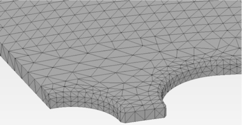
Figure 6.16Typical Mesh Generation for Part of a Vehicle Brake Disc [8].
As each of the elements is affected by forces, displacements, temperatures, etc., these effects are passed to the next element. The transmutation can then be solved by second-order partial differential equations, which were originally devised and introduced by early analytical engineers such as Rayleigh, Ritz, and Galerkin.
A typical application involves dividing the structure into a collection of subdomains. Each subdomain is then represented by a set of elements and appropriate equations. The subdomains and elements are then recombined into a global system to enable the final calculation.
Meshes can be generated with different degrees of coarseness. Critical areas of the component may have a finer mesh generated leading to a more accurate analysis. Non-critical parts of the component still require mesh generation even if only to link critical areas to each other. It should be noted that a finer mesh will lead to the requirement for greater computing power in order to cope with the larger volume of calculations.
6.8.4 Computational analysis potentials
The first step in any computational design/analysis process is to create the shape of the component. This may start as a two dimensional shape but if full advantage is to be taken of computational analysis, then a 3D shape needs to be created. It is normal, therefore, for designers to use a 3D CAD package, which usually has built-in basic analytical finite element (FE) options as standard. The basic packages would normally include stress analysis, deflections analysis, buckling analysis, heat transfer, natural frequency, and product durability. Extendable packages may include fluid flow simulation, dynamic analysis, mechanisms analysis, and many more.
6.8.5 Examples of practical applications
There follow several examples of the analysis that can be achieved with a 3D package equipped with the appropriate analytical software.
The example of a brake pedal bracket can be seen in Figure 6.17. The model shows the 3D component in which arrows indicate where the driver’s foot pressure is applied. The different colors indicate the stresses within the bracket according to the key to the right of the figure. Red-colored areas are the most highly stressed portions of the bracket, while the deep blue areas are the lowest stressed elements. Even though the red-colored areas may look seriously overstressed, the actual value depends on the setup procedure and may well be within appropriate safety limits.
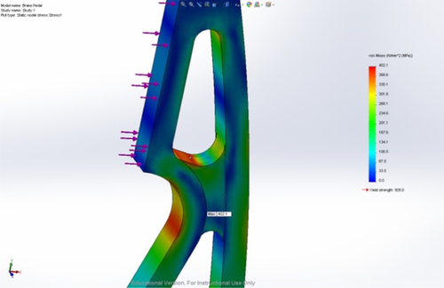
Figure 6.17Example of Brake Pedal Bracket: Stressed Component Using Finite Element Stress Analysis (Formula Student Vehicle 2013 Entry).
Plate 6.5 shows the whole pedal bracket built into the vehicle. The brake pedal is the at the center of the three pedals.
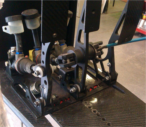
Plate 6.5Pedal Box In Situ Showing the Brake Pedal Bracket (Center) (Formula Student Vehicle 2013 Entry) [1].
Careful consideration was also given to the brakes on the vehicle. Plate 6.6 shows the brake disk in situ on the vehicle prior to being fitted with wheels. A great deal of work was applied to the brake disc in order to reduce weight and retain strength. The initial stage for the analysis of the brake disc was, first of all, to create a 3D model shown in Figure 6.18, from which the finite element mesh, Figure 6.16, could be generated.
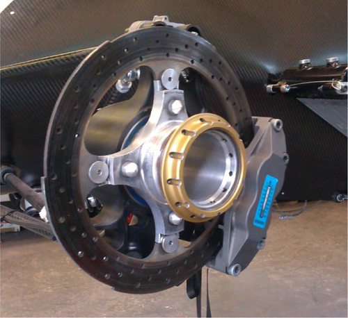
Plate 6.6Brake Disc Shown In Situ (Formula Student Vehicle 2013 Entry) [1].
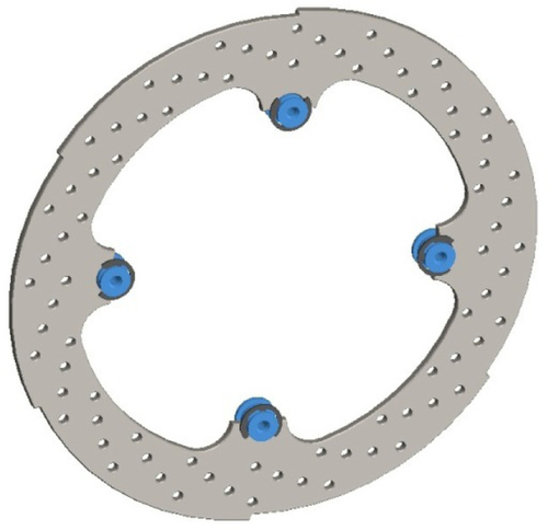
Figure 6.183D Rendition of a Brake Disc (Formula Student Vehicle 2013 Entry) [9].
Having generated the finite element mesh, several analyses can be performed on the brake disc. For instance, the thermal analysis can be seen in Figure 6.19. This shows the distribution of temperatures under certain loading conditions. Red colors indicate high temperatures and blue colors, the lowest temperatures. The temperatures as indicated may, or may not, be critical as this depends on the calibration. Analysis such as this allows the designer to determine whether excessive temperatures may warp the disc or whether the heating of the disc may be an acceptable risk.
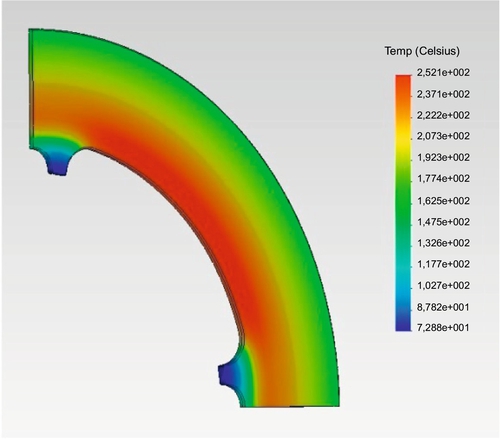
Figure 6.19Examples of Thermal Analysis of the Brake Disc (Formula Student Vehicle 2013 Entry) [9].
Computational fluid dynamics (CFD) is an extremely powerful tool that allows designers to apply fluid flow to a component within the computer environment. Since the term “fluid” refers to liquids and gases, CFD can be applied to any application where there is mass flow. Applications such as liquid flow through pipes or perhaps a flow around turbine blades are quite common. The example in Figure 6.20 is that of CFD analysis performed on the whole vehicle assembly for the FSV 2013 entry. This was executed in “ANSYS Fluent.” Here the parameter was static pressure applied to the vehicle as if it was moving through still air, but other parameters may be examined such as fluid velocities, accelerations, temperature changes, and many more.
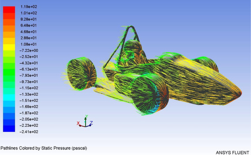
Figure 6.20Fluid Flow Analysis for the Whole Vehicle Assembly for Fluid Flow (Formula Student Vehicle 2013 Entry) [10].
Often impact behavior is the most difficult to predict, but again, using finite element methods, impact can be simulated. Figure 6.21a-e shows the progressive impact for an impact attenuator, which was intended to be fitted to the nose cone of the FSV 2013 entry. It can be seen that the attenuator is a pyramid shape where the gray disc is the external impact element. As the impact progresses, the cone gradually crushes, thus distorting the finite element mesh until in Figure 6.21e, the attenuator is completely crushed. Analysis such as this allows the designer to design an attenuator that absorbs energy progressively. Not only can the designer see the progressive shape change of the attenuator, but he can also quantify loadings and energy absorption using the scale built into each diagram.
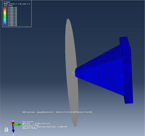
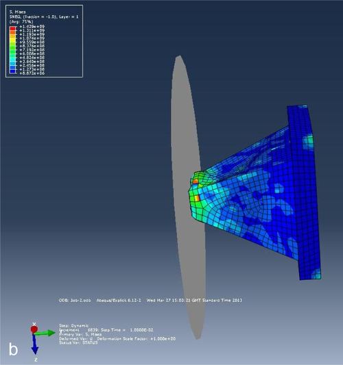
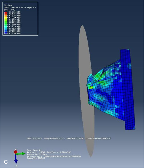
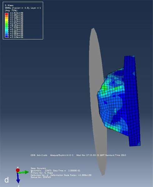
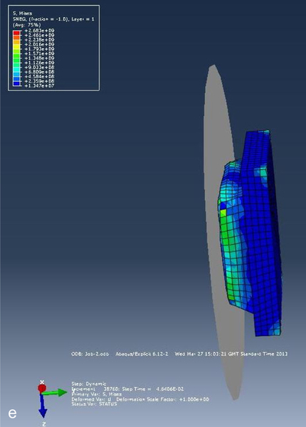
Figure 6.21(a) and (b) FEA Modelling of Progressive Impact for a Carbon Fiber Impact Attenuator [11]. (c) through (e) FEA Modelling of Progressive Impact for a Carbon Fiber Impact Atenuator [11].
Information generated within the 3D CAD system can be used for many things. As indicated in previous chapters, one of the main purposes of constructing components within the CAD system is to provide engineering drawings. Once the component is digitized within a computer’s memory, the file can be used for many other applications, analysis being just one of them.
One of the major functions of a 3D CAD system is that of assembly. Each component that is developed within the system can be assembled as if it were a manufactured component. The software creates an assembly where parts can be fitted together so that the whole assembly can be created within the computer environment and then displayed on-screen as a complete assembly. Figure 6.22 is just such an assembly where all the components have been designed within the computer environment and have then been compiled into a single assembly. Some features are built into the software, which assists in the assembly process. One such item is that of “collision detection” sometimes called “dynamic interference detection.” When two parts are fitted together, say, a shaft is larger than the hole into which it is inserted, the designer needs to know if there is a clash between the material of the shaft and the material of the hole. Dynamic interference detection will alert the designer when this happens. This ensures that when the assembly is completed as a physical prototype, the parts will fit together as originally designed.
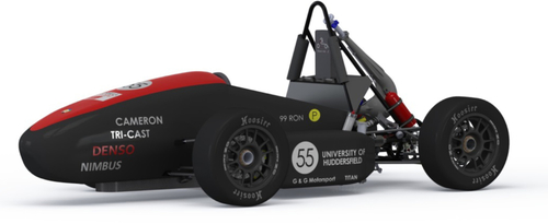
Figure 6.22Photo Rendered Image of the University of Huddersfield 2013 Entry for the Formula Student Vehicle Contest Run by the Institution of Mechanical Engineers [12].
Most clients are very pleased to receive 3D images of the product they have instigated.
To this end, 3D CAD packages have several built-in functions. Most CAD packages offer a free download of a viewer so that the customer can easily view a 3D, read-only image of the component. The marketing function may require pictures to be used with brochures, posters, etc., and to this end, rendered images can be generated. Figure 6.22 is a photographically rendered image of the FSV 2013 entry, which was used on promotional data before the vehicle was built.
6.9 Checks and Balances
The use of computer-aided analysis is relatively easy, but it is also dangerous when used by a novice, who may not understand the design challenge and, therefore, miss subtle but important elements. Checks and balances and even engineering intuition must be built into any analysis so that the designer can declare with confidence that the information generated by the computer-aided analysis is correct and accurate.
6.9.1 Computer-Aided Failure (CAF)
There is a belief among some novice engineers that if the computer can create a model, then it is correct. This assumption is very dangerous since the computer will only provide data based on the input. Furthermore, the novice may not totally understand the problem in which case his/her assumptions will be flawed from the beginning.
There have been several well-documented cases where failures have been traced back to the designer who has merely accepted information developed by computer-aided analysis. This approach could have fatal consequences if, for instance, a supermarket (Mall) roof were to collapse, which is exactly what happened several years ago. The fault was traced back to the designer who had merely accepted the results of his computer simulation.
Failure to understand and appreciate the engineering behind analysis can lead to computer-aided failure (CAF). To avoid CAF, there must be checks and balances put in place even with the most complex calculations. The checks may involve hand calculations to confirm the output from the analysis or the use of results from experimentation and a prototype’s work.
6.9.2 Stainless steel pipeline junction (by Caroline Sumner, University of Huddersfield)
Whenever a junction is placed into a pressurized pipe, the joint creates a discontinuity in the integrity of the major pipe. This is effectively a weak point and is ideal for the application of finite element stress analysis. The situation, however, is difficult to assess using hand calculations, so in this particular case, a small portion of pipe was built with an appropriate tee-junction. This can be seen in Plate 6.7. The test rig was then instrumented with strain gauges around the predicted weak area, the neck of the tee-junction as shown in Plate 6.8.
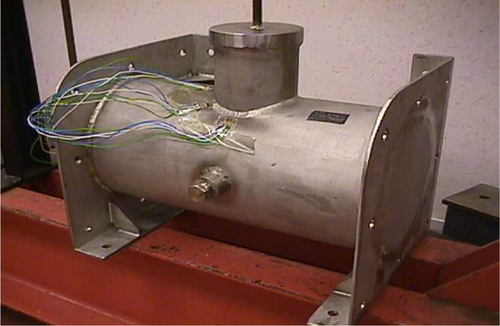
Plate 6.7Stainless Steel Pipe with Integral Tee-Joint Test Rig [1].
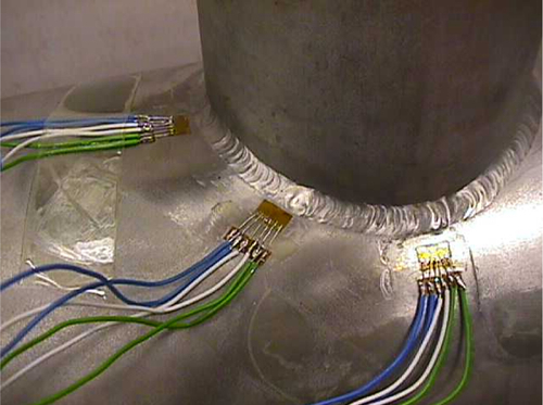
Plate 6.8Application of Strain Gauges to the Neck of the Tee-Junction [1].
The test rig was then pressurized to an appropriate test pressure whereupon the strain readings were taken and converted into values of stress (N/m2). In the meantime, the researcher was creating a 3D model and applying finite element stress analysis. The result of the analysis can be seen in Figure 6.23.
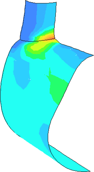
Figure 6.23Results of Finite Element Analysis on the Pressurized Tee-Junction [13].
The model shows that there is a high stress area at the neck of the tee junction. The calibration within the software determined whether this high-stress area was unsafe. It would have been dangerous, however, to accept the results of the finite element analysis without comparing those results to the results generated by the pressurizing of the test rig.
The test rig results were able to confirm the accuracy of the finite element stress analysis, effectively proving the model, which could then be used for similar applications. The reader’s attention is also drawn to the distortion in the main pipe. The entry of the tee junction creates a discontinuity in the surface of the main pipe, and the pipe distorts to compensate the spreading of the load and stresses by attempting to change the shape of the pipe. In reality, the pipe may not visibly change shape at all because of the inherent strength of the material, but the model, having zero strength may show this anomaly.
6.9.3 CFD analysis verified by a wind tunnel model (by Jay Medina, University of Huddersfield)
CFD flow analysis was applied to a fairly crude 3D model of a near-standard passenger vehicle shape so that the energy of the displaced air could be measured as the vehicle traveled at motorway speeds.
The three-dimensional model was originally created within a 3D CAD package, shown in Figure 6.24.
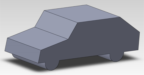
Figure 6.24Three-Dimensional Model of a Standard Passenger Vehicle [1].
The digitized version of the 3D model was then imported into the CFD package attached to the CAD software. The firsts analysis performed was to consider the location and value of the air pressure profile as it was applied to the vehicle. This analysis can be seen in Figure 6.25 and indicates the high-pressure area on the vehicle bonnet and windscreen.
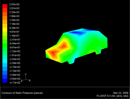
Figure 6.25Air Pressure Profile Applied to the Vehicle at a Velocity of 70 Mph [14].
It was realized that as the vehicle pushed through still air, there would be differing values of air pressure and velocity at varying heights from the ground upward. Analysis therefore created a velocity profile at 100 mm intervals upward from the road surface. Figure 6.26 shows a series of analysis “snapshots” at 100 mm intervals from the ground. It was discovered that the greater deflected air velocity and, therefore, greater energy dissipation, came from the lower levels corresponding to the least aerodynamic points on the vehicle. The output from this analysis indicated the position of the energy extraction device intended to absorb some of the energy from a passing vehicle.
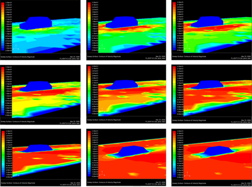
Figure 6.26A Series of Analytical Snapshots from CFD Analysis Relating to 100 mm-Height Intervals from the Road Surface [14].
The analysis appeared to be very conclusive as the red-colored areas indicated the level of maximum air disruption. Though the analysis generated a great deal of confidence, it was necessary to confirm that the analysis was correct. The consequences of the analysis being incorrect could be costly development effort spent on an energy generation device that did not work. It was, therefore, necessary to confirm the analysis by conducting wind tunnel tests.
The original 3D model shown in Figure 6.24 was fed into a rapid prototyping machine that printed 1/10 scale models. This was then used in wind tunnel tests, which indicated that the simulation model possessed some inaccuracies. After knowing the inaccuracies in the model, compensation could be made so that the model could still be used to complete the project.
6.10 Conclusion
It is essential that any computer-aided analysis be verified by whatever means. It is dangerous to take the computer-generated data as correct without this corroboration.
The designer must always be conscious that his/her design decisions and analytical results have consequences that can be related to the triple bottom line introduced in Chapter 1. To reiterate the triple bottom line, it is as follows:
First bottom line Profit
Second bottom line People and society
Third bottom line Environmental impact and sustainability
6.10.1 First bottom line
The aim of any product creation is to create value and, therefore, profit. Design decisions are aimed at increasing the value and reducing the risk. The designer should always approach the design challenge with enthusiasm and positivity, but consequences of poor design and poor analysis may lead to loss of profit and, in extreme circumstances, the demise of the company.
6.10.2 Second bottom line
Most design challenges have the intention of improving the lot of people and society in general. The consequences of poor design decisions and poor analysis could mean injury to the user and, in worst cases, even death. The responsibilities of design can be quite heavy, especially where the safety of the user is concerned.
6.10.3 Third bottom line
Awareness and consideration of the environment is an increasingly important aspect of design. The design function in the creation of new products can play an important part in reducing environmental impact. When approaching a new design challenge, the designer must develop an overview of consideration whereby the new product can be created with a reduced impact on the environment.
It can be argued that design is an art form, but Mechanical Engineering Design is an art form that is constrained by scientific principles and prediction of performance. If either or both of these two fundamentals are ignored, the consequences could be, at best, costly and, at worst, lethal.
Appendix
A6.1 Stress in a Shaft Considering Stress Concentration Factors
Determination of the stress in a gear-mounted shaft
Gear-mounted shaft with no relief groove
Find reactions
20 kN is applied in the center of the shaft. By observation, the reactions RA and RB are![]()
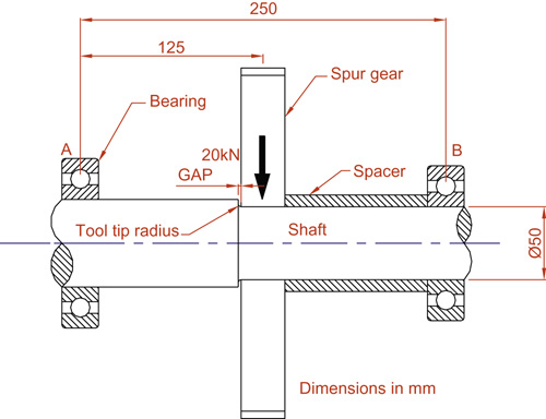
Figure A6.1Shaft Showing Tool Tip Radius [1]
Find the bending moment
The maximum bending moment occurs underneath the gear.
Assumption: the maximum bending moment occurs at the shoulder.
Bm = 0.125 × 10 × 103 = 1.25 kNm
Find the second moment of area
where D = shaft diameter of 50 mm![]()
Find the bending stress
y = 0.025 m = distance from neutral axis to extreme fibers (radius)![]()
Determine stress with relief groove
Bm = 1.25 kNm, previously calculated.

Figure A6.2Shaft Showing Relief Groove [1].
To compensate for the relief groove, the chart below can be used. See Figure A6.3. This shows stress concentration factors Ktn for circular shafts in bending with a U-shaped groove [7]. The stress concentration factors Ktn when combined within an appropriate analysis act in a manner similar to a factor of safety. The chart in Figure A6.3 requires certain minor calculations to be performed before the chart can be used. They are calculated as follows:
Key
D = major diameter of shaft = 50 mm (0.05 m)
d = diameter at the base of the groove = 44 mm (0.044 m)
r = radius at the base of the groove = 1.5 mm
Find d/D ratio
![]()
Find r/D ratio
![]()
The parameters have been marked on the chart in Figure A6.3. The Ktn can now be read as Ktn = 2.5.
This parameter can now be used to determine the nominal stress σnom.
Determine nominal stress σnom
![]()
Determine σmax
Ktn = 2.5![]()
or
σmax = σnom × Ktn = 4.6 × 106 × 2.5 = 11.5 × 10⁶ N/m2
Conclusion
The value of σmax = 11.5 MN/m2 can be considered to be the maximum stress that the shaft can undergo when such a relief groove is applied to it. Consider the maximum stress the shaft can undergo when there is no relief groove. The value of 101.9 MN/m2 is a factor of 10 greater than the maximum stress in the shaft with a relief groove. The reduction in strength is a consequence of designing into the shaft a legitimate stress raiser, but it should be considered that the analysis has allowed a precise design to be created that caters to the reduction in strength.
A6.2 Stress in Beams
In a factory refurbishment, new machinery is to be installed. In particular, large loads are to be suspended from a particular roof beam. The beam, complete with the loading regime, is shown in Figure A6.4. The beam is a standard “I” section and can be taken as being pin-jointed at each end. The beam section can be seen in Figure A6.5.

Figure A6.4Roof Beam Loading Regime [1].
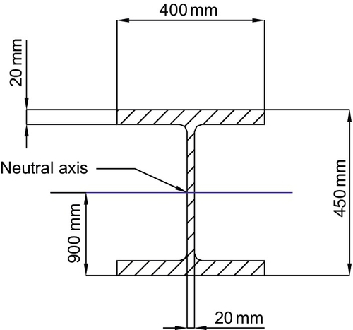
Figure A6.5Roof Beam Section [1].
As one of the engineers working on the refurbishment, your task is to analyze the beam and ensure that a minimum safety factor of 20 is applied to it when it is fully loaded.
In order to meet the criteria set out in the original brief, the analyst/designer would need to follow the following procedure:
a. Find the reactions at A and G
b. Draw the shear force diagram
c. Indicate the position of the maximum bending moment
d. Calculate the value of the maximum bending moment
e. Indicate the position of the neutral axis on a sketch of the beam section
f. Determine the second moment of area for the section
g. Determine the maximum bending stress in the beam
h. If the ultimate tensile strength of the cast iron material is 150 MN/m2, determine the factor of safety. State whether the actual factor of safety complies with the design factor of safety.
a. Find the reactions at A and G
Clockwise moments = anticlockwise moments
To find RA
Moments about RG
RA × 5 = (2 × 5) + (4 × 4) + (4 × 2.5) + (3 × 1.7) + (3 × 0.4)![]()
To find RG
Upward forces = downward forces
RA + RG = 2 + 4 + 4 + 3 + 3
RG = 16 − 8.46 = 7.54 kN
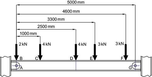
Figure A6.6Roof Beam Loading Regime [1].
b. Draw the shear force diagram
c. The maximum bending moment is indicated in Figure A6.7
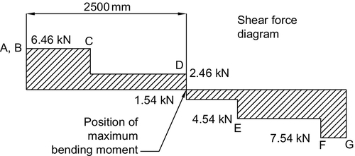
Figure A6.7Shear Force Diagram [1].
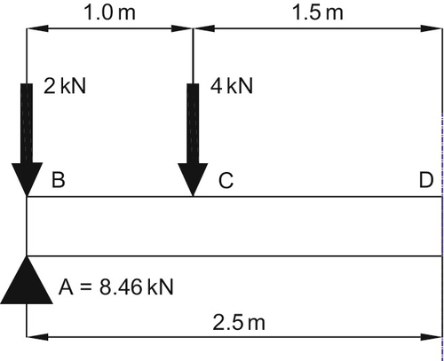
Figure A6.8Bending Moment Space Diagram [1].
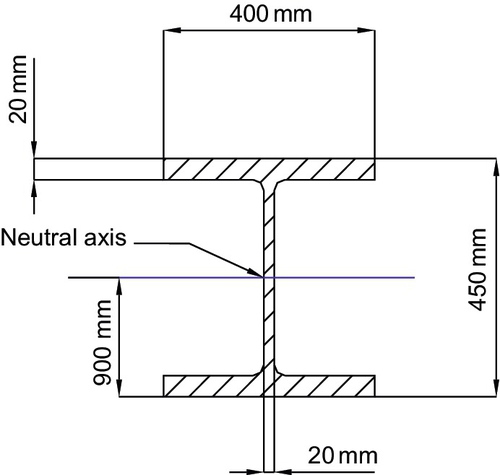
Figure A6.9Sectional View of Intended Beam [1].
d. Calculate the value of the maximum bending moment
Clockwise moments = anticlockwise moments
Clockwise moments are + ve
Moments about D
MD = (8.46 × 2.5) − (2 × 2.5) − (4 × 1.5)
MD = 21.15 − 5 − 6 = 10.15 kNm
e. Indicate the position of the neutral axis on a sketch of the beam section
f. Determine the second moment of area for the section![]()
![]()
IUpper flange = ILower flange = 3.7 × 10− 4 m4![]()
ITotal = IUpper flange + ILower flange + IVertical web = 8.39 × 10− 4 m4
g. Determine the maximum bending stress in the beam![]()
![]()
h. Find the factor of safety![]()
Calculated FoS is above a design FoS of 20 and is therefore adequate
A6.3 Torsion in a Shaft
A torsion meter whose schematic is shown in Figure A6.10 is attached to a ship's propeller shaft. The torsion meter operates by comparing the position of two flanges set a certain distance apart on the shaft. The torsion meter is set so that the flanges and, therefore, the reading surfaces are set 3 m apart. The readings therefore allow the engineers to judge whether the shaft is being overstressed in torsion. The diesel engine is able to apply a maximum torque of 25 kNm to the shaft. As one of the engineers developing the torsion meter for this particular ship, you are required to calculate the stresses and torsional displacement to confirm the accuracy of the torsion meter.
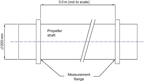
Figure A6.10Measurement Setup for the Torsion Meter [1].
The parameters of the shaft are as follows:
outside diameter: 200 mm
inside diameter: 192 mm
distance between measurement points: 3 m
material: medium carbon steel, modulus of rigidity = G = 80 GN/m2
maximum torque = 25 kNm.
The design engineer is required to follow the procedure set out here in order to fulfill the project requirements.
a. Find the polar second moment of area for the shaft.
b. Find the angle of twist between the measurement points of the torsion meter in radians.
c. The angle of twist in the shaft should not exceed 3° in any 3 m length. Compare the calculated value with the design value and indicate if the system is within designed parameters.
d. Determine the shear stress in the shaft caused by the applied torque of 25 kNm.
e. The ultimate shear strength for the propeller shaft material is 270 MN/m2. Find the factor of safety.
f. The factor of safety set by the designers is 3. State whether the stresses in the shaft meet this criterion.
g. Find the total angle of twist between the engine and the propeller if the distance is 13 m.
a. Determine the polar second moment of area for the shaft
Outside diameter = 200 mm
Inside diameter = 192 mm
G = 80 GN/m2
Torque = 25 kNm![]()
b. Determine the angle of twist between the measurement points of the torsion meter in radians.
Length = 3.0 m, G = 80 GN/m2
From![]()
![]()
c. The angle of twist in the shaft should not exceed 3° in any 3 m length. Compare the calculated value with the design value and indicate if the system is within designed parameters.![]()
The shaft will twist 2.27°, which is less than the maximum allowable twist of 3°.
The shaft is within design parameters.
d. Determine the shear stress in the shaft caused by the applied torque of 25 kNm
Torque = 25 kNm, r = 0.1 m
From![]()
![]()
e. Determine the factor of safety if the ultimate shear strength is 270 MN/m2
f. The factor of safety set by the designers is 3. State whether the stresses in the shaft meet this criterion.
The new safety factor is 2.84, which is adequate to meet the design factor of safety of 3
g. Determine the total angle of twist between the engine and the propeller if the distance is 13 m.
Angle of twist over a 3 m length = 2.27°
Angle of twist over ![]()
A6.4 Dynamics of Solid Bodies/Mechanics: Bicycle Parameters
You are a designer of bicycles and have been tasked with performing analysis relating to the worst conditions that a particular size of bicycle will see in service. They relate to the deceleration involving brake efficiency and acceleration involving the rider’s ability to inject energy. The analysis thus performed will be used to improve the new bicycle design. Please see Figure A6.11 for masses. Figure A6.12 shows the wheel dimensions.

Figure A6.11Bicycle Mass Elements [1].
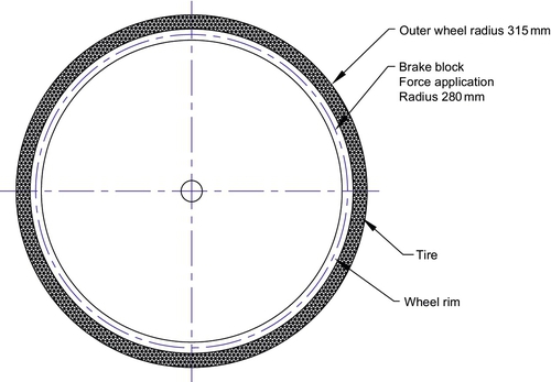
Figure A6.12Wheel Dimensions [1].
The following parameters prevail:
| General | |
| Rider mass | 95 kg |
| Bicycle mass | 10 kg |
| Wheel radius road/tire interface | 315 mm |
| Radius of brake shoes | 280 mm |
| Deceleration analysis | |
| Initial velocity u | 40 km/h |
| Final velocity v | 0 |
| Stopping distance | 20 m |
| Acceleration analysis | |
| Pedal radius | 200 mm |
| Pedal sprocket diameter = drive wheel sprocket diameter |
The design engineer is required to follow the procedure set out here in order to fulfill the project requirements.
a. Find the deceleration in m/s2 when bringing the bicycle to a halt. Refer to the parameters specified earlier.
b. Determine the value of the deceleration force at the road/tire interface assuming that the entire braking force is delivered to one wheel only.
c. Determine the force required at the brake block noting the difference between the road/tire interface radius and the brake block radius (in N).
d. The rider now accelerates by standing on a pedal with all his mass as indicated in Figure A6.13. Determine the driving force at the rear wheel at the road/tire interface (N). The pedal radius is 200 mm and the road/tire interface radius is 315 mm. Assume the drive sprocket and the driven sprocket are the same diameter.
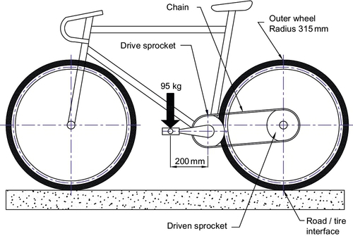
Figure A6.13Pedal-Wheel Relationship [1].
e. Determine the acceleration of the bicycle and rider in m/s2.
f. Determine the final velocity of the bicycle if the initial velocity is zero and the acceleration is maintained for 1.6 s.
g. The resistance to motion is a combination of the rolling resistance of tires, bearing friction, and aerodynamic resistance. The resistance to motion of the bicycle and rider can be taken as 2.5 N/kg. Find the total resistance to motion.
h. Find the work done in 20 min if the maximum velocity of 9 m/s is maintained.
i. Find the power applied by the rider during the maximum velocity (9 m/s) period.
a. Find the deceleration in m/s2![]()
Final velocity v = 0
Stopping distance S = 20 m
From v2 = u2 + 2aS
Transpose for a![]()
Note that -ve indicates deceleration
v = 0
b. Determine the value of the deceleration force at the road/tire interface (N)
Mass = rider + bicycle = 95 + 10 = 105 kg
From F = ma![]()
c. Determine the force required at the brake block
Wheel torque = brake torque
Force at wheel × wheel radius = force at brake × brake radius
Fw × Rw = Fb × Rb![]()
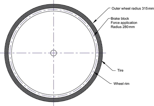
Figure A6.14Wheel Dimensions [1].
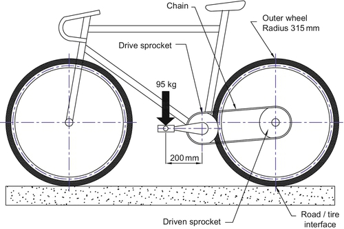
Figure A6.15Bicycle Relative Components [1].
d. Determine the driving force at the rear wheel at the road/tire interface (N)
For equilibrium
Torque at pedal = Torque at wheel
Note: 95 kg × 9.81 m/s2 = 932 N
Fp × Rp = Fw × Rw
e. Determine the acceleration of the bicycle and rider in m/s2
Mass = Rider mass + bicycle mass = 95 + 10 = 105 kg
From F = ma,![]()
![]()
f. Determine the final velocity of the bicycle
From v = u + a × t
g. Find the total resistance to motion![]()
![]()
h. Find the work done in 20 min
WD = resisting force × distance![]()
i. Find the power applied by the rider during the maximum velocity (9 m/s) period![]()
Power = force × velocity![]()
Alternative![]()
A6.5 Inertias and Power Prediction
A diesel engine is configured to drive a rotating drum as shown in Figure A6.16. In operation, the engine is instantaneously coupled to the drum via a friction clutch.
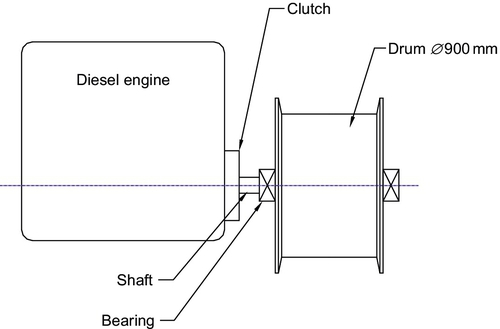
Figure A6.16Diesel Engine, Clutch, and Winding Drum Configuration [1].
The moment of inertia of the engine is equivalent to a mass of 25 kg acting at a radius of gyration of 393 mm. The engine rotates at 200 rev/min before engagement with a drum winch through the clutch.
The drum has a mass of 60 kg acting at a radius of gyration of 406 mm and is initially at rest.
The drum is the winding end of a winch having a rope wrapped around its diameter of 900 mm. It is designed to lift 1000 kg pallets through the floors of a warehouse.
a. Determine the moment of inertia of the engine
b. Determine the moment of inertia of the drum
c. Determine the combined angular velocity in rev/min immediately after connection. Assume the drum and the engine do not separate after connection
d. Determine the power required at the engine to lift a 1000 kg pallet using the combined angular velocity calculated in part (c). Assume no losses in the system.
(a) Determine the moment of inertia of the engine![]()
![]()
(b) Determine the moment of inertia of the drum![]()
![]()
![]()
(c) Determine the combined angular velocity in rev/min immediately after connection.
ωD = zero (initial angular velocity of drum)
Using the principle of conservation of momentum
Momentum before connection = momentum after connection![]()
(IE × ωE) = (IE + Idrum)ωcombined
ωcombined = combined angular velocity![]()
(d) Determine the power required at the engine to lift a 1000 kg pallet
Find torque at the drum
Torque = Force × drum radius![]()
Find power
![]()
A6.6 Dynamics: Vibration Isolation
Diesel engine motive power is usually used for large items of plant such as that shown in Figure A6.17. Such large engines need to be placed on engine mounting systems so that the induced vibrations are isolated from the chassis, thus preventing unwanted vibrations reaching sensitive equipment and personnel. Diesel engines are normally mounted on four vibration isolators, also shown in the schematic in Figure A6.17. In this case, assume the engine mass is 2600 kg, which is distributed evenly between the four isolators. The speed of rotation of the engine is 1800 rev/min.
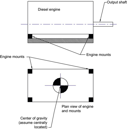
Figure A6.17Engine Mount Arrangement for Large Diesel Engine [1].
Considering only oscillation in the vertical direction and using the isolation efficiency graph in Figure A6.18, calculate the individual stiffness of the isolators if the isolation efficiency is to be 90%. Assume that the isolators are identical and that damping can be neglected for this selection process.
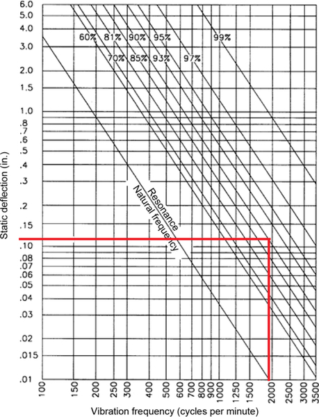
Figure A6.18Isolation Efficiency Graph [8] (Note 1 in. = 25.4 mm).
Find load on each isolator
![]()
![]()
Find the deflection from the Isolation Efficiency graph (Fig A6.18)
rev/min (cycles/minute) = 1800 rev/min
Isolation 90%
Insert vibration frequency and read deflection from the Graph
Deflection 0.12 in.
Deflection (metric) 0.12 x 25.4 = 3.05 mm (0.00305 m)
Find spring stiffness
![]()
The spring stiffness can now be used to select an appropriate mount from a supplier of anti-vibration mounts
A6.7 Structural Design of the Denby Dale Pie Cooker
In the year 2000, the Denby Dale Pie cooker took the form of a welded steel structure with 24 compartments containing the stew. Figure A6.19 shows the layout of part of the structure excluding the compartments.

Figure A6.19Basic Structure of the Denby Dale Pie Cooker [1].
The 2004 attempt at the “Biggest Pie in the World” was to have a mass of 12 tons and cooked in a specially made “pie dish.”
The whole structure was considered as a simply supported beam, 12 m long, whose total mass was 6000 kg and which was treated as a uniformly distributed load (UDL) of 4900 N/m.
The designers were required to ensure that the structure was safe by performing stress analysis and determining the factor of safety. The beam can be taken as simply supported with a loading regime as shown in Figure A6.20.
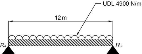
Figure A6.20Loading Regime for the Denby Dale Pie Cooker [1].
The designers followed the route given here by calculating the following:
a. The position of the neutral axis of the structure.
b. The reactions at the supports.
c. The shear force diagram indicating the position of the maximum bending moment.
d. The maximum bending moment
e. The total second moment of area for the beam
f. The maximum stress at the position of the maximum bending moment
g. The factor of safety given that the material used has an ultimate tensile strength (UTS) of 480 MN/m2
a. The position of the neutral axis of the structure.
The structure is 1.2 m high and is uniform
By observation, the neutral axis N/A acts at 0.6 m from the base at the center of the section
b. The reactions at the supports.
Clockwise moments = anticlockwise moments
Moments about RB
RA × 12 = [(4900 × 12) × 6]![]()
![]()
c. The shear force diagram indicating the position of the maximum bending moment.
d. The maximum bending moment
Clockwise moments = anticlockwise moments
Moments about the center of the beam![]()
e. The total second moment of area for the beam
From![]()
Find Ixx for a single beam element as shown in Figure A6.22
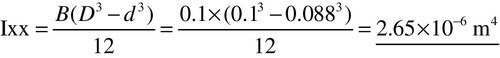
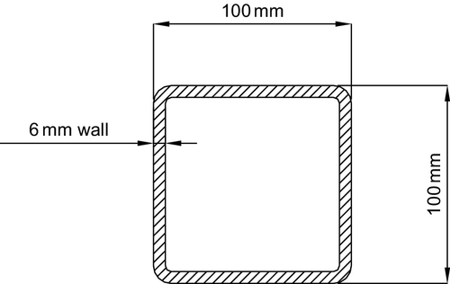
Figure A6.22Cross-Section of a Single Beam Element [1].
Find cross-sectional area
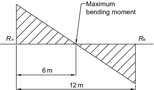
Figure A6.21Shear Force Diagram Showing Position of Maximum Bending Moment [1].
![]()
Find total second moment of area IxxT
Refer to Figure A6.23
From![]()
![]()
![]()
Second moment of area for a single column IxxSC![]()
But there are three columns![]()
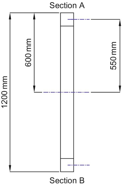
Figure A6.23Structure of One Single Column Within the Fabrication [1].
f. The maximum working stress σw at the position of the maximum bending moment,
where y = N/A to extreme fibers = 0.6 m
From![]()
g. The factor of safety given that the material used has an ultimate tensile strength (UTS) of 480 MN/m2 and is considered to be very safe
A6.8 Heat Transfer
Denby Dale Pie: maximum rate of ingredients addition
During the cooking of the pie, it was essential that the ingredients were added to the stew in a precise fashion so that temperatures did not fall below 65 °C. This would trigger the growth of the C. perfringens bacterium. This is the bacterium that causes food poisoning and typically causes victims to develop diarrhea and sickness. It was, therefore, imperative that the stew was cooked in such a way as to avoid the growth of the bacterium.
The cooking process involved heating the ingredients of each of the twenty four vats to 100 °C, then adding further ingredients such as chopped potatoes, onions, and seasoning. It was the task of the designer to calculate, using the principles of heat transfer, the mass of ingredients that could be added before the stew temperature was reduced to 65 °C. The parameters were as follows:
| Temperature of frozen ingredients | − 4 °C |
| Specific heat capacity of stew (derived through experimentation), C | 4200 J/kg K |
| Temperature of main body of stew | 100 °C |
| Mass of main body of stew | 500 kg |
Determine the Energy Capacity of 500 kg of Boiling Stew
Cp = C × mass × (temperature change)
where Cp = energy capacity (J)![]() .
.
Determine the mass that can be added
Determine the mass of ingredients that can be added to bring the general temperature down to 65 °C.
Conversely, determine the mass that will increase the temperature of the ingredients to 65 °C using the available energy of 210 MJ.
Cp = 210 MJ
t1 = − 4 °C
t2 = 65 °C
C = 4200 J/kg K
From
Cp = C × mass × (t2 − t1)
isolate mass![]()
The mass that could be added to each vat was 724 kg. This was more than was needed in total for each individual vat. In practice, no more than 50 kg of ingredients were added at any one time, thus keeping the stew temperature well above the minimum 65 °C.
References
[2] www.weldingweb.com 2013.
[3] The Stadium, Architecture for the New Global Culture, Periplus Editions, Hong Kong, 2005.
[4] D. Warburton, Final Year undergraduate design exercise, Huddersfield University, UK, 2012.
[5] Dr. Leigh Fleming, University of Huddersfield.
[6] Michele Bandini. E-mail: [email protected]: www.peenservice.it.
[7] Pilkey WD, Pilkey DF. Peterson's Stress Concentration Factors. third ed. Hoboken NJ: John Wiley & Sons; 2008.9780470 048245.
[8] Thompson WT. Theory of Vibrations. Chelrenham UK: Nelson Thornes Ltd.; 2012.
[9] Barron Luke, University of Huddersfield, UK, 2013.
[10] Hague S, University of Huddersfield, UK, 2013.
[11] King Oliver, University of Huddersfield, UK, 2013.