
Learning Based on Logic
Logical inference using knowledge represented by predicate logic and inference rules does not seem to generate any new information or have anything to do with learning. However, when we try to understand the structure that is buried in a large amount of complicated knowledge, we can regard a system for organizing knowledge by logical inference as generating new knowledge that we have not seen before. Also, a system based on logic can be used for algorithms that actually generate new information by embedding learning methods, such as generalization and specialization, into logical inference. We generally refer to learning based on logical inference as learning based on logic. In this chapter, we will explain various learning algorithms based on logic.
8.1 Explanation-Based Learning
Suppose we have a concept c and its positive instance, a. The fact that a is a positive instance of c corresponds, from the viewpoint of logic, to the fact that c can be proved from a. For example, with well-formed formulas
the fact that taro is an animal is proved from the fact that taro is a human being, so we can think of taro as a positive instance of an animal. This logical relation between concepts and instances can be looked at as saying that the formulas (8.1) are a logical “explanation” of the concept animal(X). Also, if we rewrite (8.1) using the substitution {T/taro} as
we have the generalization that not only taro but also any human being is a positive instance of an animal.
Generalizing a logical explanation like this can be thought of as a kind of learning. Learning in this sense is called explanation-based learning. We will describe this kind of learning in this section.
(a) Explanation-based generalization
Explanation-based generalization is intuitively, as suggested in (8.1) and (8.2), the process of generalizing the logical relation between a concept and its positive instance by replacing constant symbols in well-formed formulas with variable symbols.
Explanation-based generalization can be formulated as a general algorithm using an algorithm for theorem proving. Let us first explain such an algorithm by an example.
Suppose the system wants to learn the relation between the concept “resort” and its positive instance. Suppose further that it knows that a resort is a place with nice weather and is good for a vacation. In other words
is given as a goal concept. Here ↔ is the logic symbol representing → and ←. Next, suppose that a description of one positive instance of the goal concept is given. For example, suppose we give a description of “sapporo” as a positive instance of “resort.” The following conjunction (or equivalently a set) of ground literals is given:
Furthermore, as the domain theory, we give the following set of logic formulas:
Using the formulas in (8.5) we can prove resort_place (sapporo) (the left side of (8.3)) from the description of “sapporo” given in (8.4). In other words, “sapporo” satisfies the goal concept “resort.”Figure 8.1 shows the proof process using a proof tree.
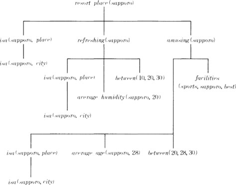
A proof tree that shows the logical relation between a goal concept and one of its positive instances is called an explanation structure for the goal concept. In order to do generalization based on explanation, we first replace constant symbols in this explanation structure with variable symbols. For example, we propagate the substitution {Z/sapporo} downward from the root node of the tree in Figure 8.1 in order to generalize the constant symbol “sapporo” to Z. For example, resort_place(sapporo) is generalized to resort_place(Z), and in the lower nodes we get isa(Z, place), refreshing(Z), amusing(Z) as shown in Figure 8.2, where at each node the substitution into the formulas (8.3), (8.4), (8.5) is repeated. For example, at nodes under the node refreshing(Z) in Figure 8.2, (8.5) provides the substitution {H/20}. As a result, the necessary substitution for obtaining a generalization of the whole proof tree shown in Figure 8.2 is {Z/sapporo, H/20, A/28}.
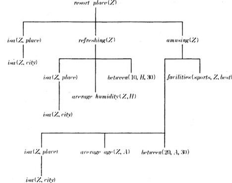
The proof tree shown in Figure 8.2 demonstrates that the well-formed formula at the root node can be proven from the conjunction of its leaves. That is,
Formula (8.6) generalizes and explains the goal concept resort_place(Z) using only predicates included in the description of the positive instance (8.4) (except for the predicate between). (8.6) can be read as “a city where the average humidity is between 10% and 30% and the average age of the residents is between 20 and 30 years old and there are good sports facilities is called a resort.” The description (8.4) of the positive instance “sapporo” satisfies (8.6). (8.6) gives a sufficient condition for given data to be a positive instance of the goal concept.
In the above example, as in (8.6), the original concept can be described using only the predicates that appear in the description of the positive instance (except for the predicate between). However, this is generally not the case. Rather, in most cases the goal concept can only be explained using predicates that appear in the domain theory, but not in the positive instance. Finding these predicates is an interesting learning problem on a computer. The relation between the goal concept and a positive instance can be seen as a constraint on using some data as a positive instance of the goal concept. This constraint is generally called an operationality criterion (for the goal concept).
Let us formulate, in general terms, the algorithm for the explanation-based generalization that we explained above. First, let us make the problem clear.
[The problem of explanation-based generalization]
(1) goal concept: a well-formed formula that describes the concept to be learned
(2) positive instance: a set of ground literals that describe a positive instance of the goal concept
(3) domain theory: a set of well-formed formulas that are related to the positive instance and the goal concept
(4) operationality criterion: a constraint on the positive instance for being usable as a positive instance of the goal concept, the problem is to find
(5) a sufficient condition: a sufficient condition that is a well-formed formula satisfying the operational criterion and makes the given positive instance a positive instance of the goal concept.
For example, the operationality criterion of the problem in the “resort” example specifies that “a sufficient condition should be described only by the predicates that correspond to literals appearing in the positive instance.”
Now, the basic algorithm for solving the above problem is described below. However, the following algorithm can sometimes fail. An example of this failure and its recovery will be explained in (b).
Algorithm 8.1
(explanation-based generalization)
[1] If the well-formed formula describing the goal concept satisfies the operational criterion, then stop. In this case, we do not need to generate a new sufficient condition by generalizing the positive instance. Otherwise, go to [2].
[2] Generate the explanation structure E of the goal concept c using the set of ground literals describing the positive instance, L, and the domain theory, M. E is the proof tree that corresponds to the proof of L ∪ M ![]() c, where L ∪ M is a set of axioms.
c, where L ∪ M is a set of axioms.
[3] Find a substitution θ that makes c = n0θ for c and the root node n0 of E, and propagate this substitution downward from no to all the nodes of E.
[4] Do [3] for each node of E (other than the root node). If, for the literal l at each node, there is a literal X in M such that a substitution θ exists that makes l = Xθ, propagate the substitution using those literals. If such a literal X does not exist, then leave l as is.
[5] Construct the well-formed formula
where C is the conjunction of the leaves in the generalized explanation structure that was obtained in [4]. This well-formed formula describes a desired sufficient condition.
(b) Generalization using upward propagation
The algorithm for explanation-based generalization described in (a) repeats the substitution at each node downward from the root node of the proof tree. There are some cases where this algorithm does not work.
We will consider these cases and explain how to deal with them using an example. Suppose we have the following explanation-based generalization problem.
| (1) | goal concept: | love(A,B) |
| (2) | positive example: | selfish(hanako) |
| good_point(good_proportion) | ||
| get(hanako, good_proportion) | ||
| (3) | domain theory: | sympathetic(P, Q) ∧ attractive(R) ∧ have(P, R) |
| → love(P, Q) | ||
| selfish(X) → sympathetic(X, X) | ||
| good_point(Y) → attractive(Y) | ||
| get(Z, W) → have(Z, W) |
(4) operationality criterion: The sufficient condition is described only using predicates that correspond to literals appearing in positive instances, find
(5) sufficient condition: A well-formed formula that satisfies the operational criterion and gives a sufficient condition for the positive instance to be a positive instance of the goal concept.
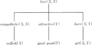
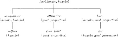
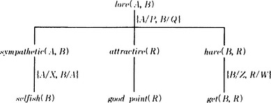
First, if we apply Algorithm 8.1, we obtain in [2] the explanation structure shown in Figure 8.3. Then, in [3] and [4], we try to generate a generalized explanation structure. For example, c = noθ holds with the substitution θ = {A/hanako, B/hanako} for the goal concept of the problem, c = love(A, B), and the root node of the proof tree shown in Figure 8.3, no = love(hanako, hanako). So, we propagate the substitution downward using θ. Similarly, if we generalize the explanation structure in Figure 8.3, we obtain the generalized explanation structure shown in Figure 8.4 using the substitution {A/hanako, B/hanako, R/good_proportion}. Figure 8.4 also shows the substitutions for deriving the tree. Note that the substitution is repeated at each node, making use of the domain theory.
Next, from the conjunction of the leaves of the generalized explanation structure in Figure 8.4, we obtain the following well-formed formula:
However, the interpretation of (8.7) is “if B is selfish and has some good point, any A loves B.” This is not what we expected.
This result is due to the fact that the goal concept, love(A, B), is too general compared to the domain theory used in generating the explanation structure in Figure 8.3. So, we try to generalize the appropriate goal concept by propagating the substitution upward from the leaves of the explanation structure, inverting the direction of propagation in [3], [4] in Algorithm 8.1.
For example, if we apply the domain theory to the leaves of the explanation structure in Figure 8.3 and propagate the substitution {X/hanako, Y/good_proportion} upward, we get the explanation structure shown in Figure 8.5. By using this explanation structure, we get the following new well-formed formula representing the relation between the goal concept and the positive instances:
This expression can be interpreted as “If X is selfish and has some good point, X loves himself.” Also, using the formula (8.8), the goal concept, love(X, X), can be explained only using the predicates appearing in the description of the positive instance, and thus (8.8) satisfies the operationality criterion.
By generalizing the method explained above by example, we can change the algorithm in the following way:
Algorithm 8.2
(improved algorithm for explanation-based generalization)
We change [3] and [4] in Algorithm 8.1 to the following:
[3]’ Find a substitution θ that makes X = lθ for each leaf, l, of E and literal X in L ∪ M, and propagate θ to all the nodes of E upward from l. If such a substitution does not exist, leave l as is.
[4]’ Do [3] to each node of E (other than leaves).
(c) Generalization by unification of Horn clauses
Upward propagation of substitutions in a proof tree is actually a special case of unification used in logical inference. On the other hand, unification can easily be done by executing a Prolog program if we limit the representation of formulas to Horn clause logic. Actually, full explanation-based generalization can easily be done using Prolog as long as we limit our representation to Horn clauses. We will describe a method of explanation-based generalization under Horn clause logic, using unification in Prolog.
First, let us remember that the following two trees were generated in our algorithm for the explanation-based generalization:
(i) A proof tree for proving the goal concept from a positive instance and domain theory. This tree does not contain variables.
(ii) A generalized proof tree that replaces the goal concept for the root node of the proof tree (i) with the original goal concept (that includes variables) and propagates this substitution to all the nodes of the tree.
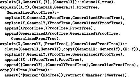
These trees can be generated all at once using the Prolog program shown Figure 8.6. By executing this program, the proof trees (i) and (ii) are substituted into ProofTree and GeneralizedProofTree, respectively. Then, the desired sufficient condition can be obtained as the Horn clause whose head is the root node and whose body consists of the leaves of the proof tree that is substituted into GeneralizedProofTree. For example, the problem explained in (b) can be represented in Horn clause logic and can be rewritten as the Prolog program in Figure 8.7.
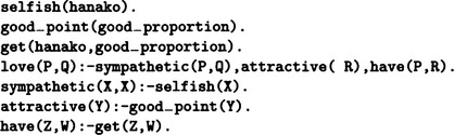
Now, for this program, let us compare the goal concept with constants, love(hanako, hanako), and the goal concept with variables love(A, B). For that, it is sufficient to generate the proof trees (i) and (ii) at the same time by using the unification {A/hanako, B/hanako}. We use the following goal:
If we generate the two proof trees (i) and (ii) using the goal (8.9) and the programs in Figure 8.6 and 8.7, we obtain the output shown in Figure 8.8. _4 and _36 are Prolog variables. From Figure 8.8, we notice that the variables in (8.9), A and B, are unified to the same variable _4 and there occurred no problem of substitution such as described in (b). Using the leaves of the proof tree (ii) obtained in Figure 8.8 and the goal concept after the unification, we obtain the following Horn clause:
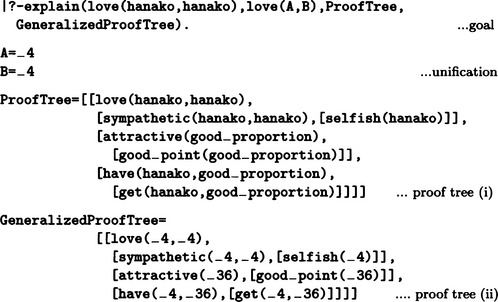
This is the same as the sufficient condition (8.8) that was obtained in (b).
8.2 Analogical Learning
(a) Analogical reasoning
Just as a cat eats a rat, a lion eats a zebra. We can represent this relation as follows where eat and smaller_than are predicate names:
What should be in the place of ? in (8.13) can be easily inferred from the other three predicates. From (8.10) and (8.11), a cat corresponds to a lion and a rat corresponds to a zebra. From (8.12) a cat and a lion are related by “smaller-than,” so we can infer that a zebra is related to a rat by “smaller-than.” This kind of inference based on relations among objects is called analogical reasoning.
In analogical reasoning, we can make an inference even when there is not sufficient knowledge about an object to be inferred. Actually, we can generate new knowledge as the result of analogical reasoning. For example, though we have no knowledge of the size of a rat and a zebra before the above reasoning, the fact that a rat is smaller than a zebra can be inferred. This characteristic of analogical reasoning suggests that such reasoning is a kind of learning for obtaining new knowledge. If analogical reasoning is done in order to obtain new knowledge, such reasoning is called learning by analogy.
(b) Framework for learning by analogy
Let us make a relatively formal definition of learning by analogy. First, suppose we have two knowledge bases, B and T. We assume that each element of B and T can be represented as a finite set of ground literals. For example, let B be the world of the solar system and T the world of atoms, and let us choose an element of B, earth, and an element of T, electron. These elements can be represented as the following sets of ground literals:

Now, let us give the following definition:
Definition 1
(similarity relation) Suppose P1 and P2 are finite sets of predicates and q1 ∈ P1, q2 ∈ P2 are predicates whose names are the same. Then the pair 〈q1, q2〉 is said to be in a similarity relation on P1 × P2.
For example, 〈attracted(earth, sun), attracted(electron, nucleus)〉 is in a similarity relation on D1 × D2.
Now, for ![]() and
and ![]() , the set of the predicates that are in a similarity relation on B × T can be written as
, the set of the predicates that are in a similarity relation on B × T can be written as
where ![]() are terms. For example, in the above example, for
are terms. For example, in the above example, for ![]()
There are corresponding relations between the pairs of terms xjk and yjk (k = 1, …, mj) for each pair of predicates in the similarity relation, p(xj1, …, xjmj) and p(yj1, …, yjmj), j = 1, …, n. For example, in (attracted(earth, sun), 〈attracted(electron, nucleus)〉, the constant earth corresponds to electron and sun corresponds to nucleus.
If we substitute the same variable Ajk into the corresponding terms xjk and yjk, (8.14) becomes
For example, for PD1 × D2 we have
where in order to restore QD1 × D2 to PD1 × D2’ we can use the pair of substitutions
Now, let’s summarize all of this. Let us write QB×T simply as Q and let v(Q) be the set of variable symbols included in Q. Also, let us define the substitution θ as
We give the following definition:
Definition 2
(partial match) Suppose, ![]() and
and ![]() and T are finite sets of ground literals without common constant symbols. If, for a set of literals in
and T are finite sets of ground literals without common constant symbols. If, for a set of literals in ![]() and Qθ and v(Q)θ are one-to-one relations, (Q, θ) is called a generalized partial match or simply a partial match of β and r, or β x r.
and Qθ and v(Q)θ are one-to-one relations, (Q, θ) is called a generalized partial match or simply a partial match of β and r, or β x r.
For example, in the previous example, if we let (8.15) and (8.16) be Q and θ, respectively, (Q, θ) is a partial match for D1 × D2. For a given pair of sets, β × r, there can be more than one partial match. A partial match is a (generalized) common part of the two sets; however, it can be a small part or a bigger part including the small part. Suppose we have
Then (Q′θ′) is a partial match for D1 × D2, but intuitively it is smaller than (Q, θ). Now, let us define a partial order on partial matches as follows:
Definition 3
(partial ordering) Let (Q, θ) and (Q’, θ′) be two partial matches for a pair of given sets, β × T. If there exists a substitution ξ such that ![]() , and
, and ![]() for any
for any ![]() , we say that (Q,θ) is bigger than (Q’, θ′) and write (Q,θ) ≤ (Q’, θ′).
, we say that (Q,θ) is bigger than (Q’, θ′) and write (Q,θ) ≤ (Q’, θ′).
Definition 4
(maximal partial match) If, for partial matches (Q, θ) and (Q’,θ′) for ![]() whenever
whenever ![]() , we say that (Q, θ) is a (generalized) maximal partial match for β × T.
, we say that (Q, θ) is a (generalized) maximal partial match for β × T.
In the example above, the partial match (Q, θ) defined in (8.15) and (8.16) is a maximal partial match for D1 × D2. But the partial match (Q’, θ′) given in (8.17) and (8.18) is not maximal. Note that a maximal partial match for the same pair of sets is not unique.
Now, let us extend the notion of a partial match for a pair of sets, ![]() , to a partial match for a pair of relations. Suppose
, to a partial match for a pair of relations. Suppose ![]() are in relation b12. For example, if we have
are in relation b12. For example, if we have
b12 is the relation “A small object is moving around a big object.”
Suppose, for ![]() and
and ![]() , we know a maximal partial match m for
, we know a maximal partial match m for ![]() . Let us consider another set
. Let us consider another set ![]() such that m also is a maximal partial match for
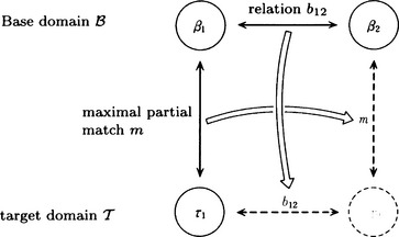
such that m also is a maximal partial match for ![]() and the relation between r1 and r2 can be replaced by the relation b12. We now define learning by analogy formally as follows:
and the relation between r1 and r2 can be replaced by the relation b12. We now define learning by analogy formally as follows:
Definition 5
(learning by analogy) Suppose, for ![]() , and a relation b12 on
, and a relation b12 on ![]() and a maximal partial match m for
and a maximal partial match m for ![]() is known. Then, finding
is known. Then, finding ![]() such that
such that ![]() and m is a maximal partial match for β2 × r2 is called learning by analogy.
and m is a maximal partial match for β2 × r2 is called learning by analogy.
The relation among β1, β2, T1, and T2 in Definition 5 is shown in Figure 8.9. According to the above definition, learning by analogy looks for knowledge T2 in T, which can be newly related to the already known knowledge b12 and m. As shown in Figure 8.9, we call the already known knowledge domain B the base domain and the unknown knowledge domain T the target domain.
For instance, in the previous example (8.19), let us make
and consider the following maximal partial match for β1 × T1:

By computing b12θ2, we obtain
So, we can set
In Definition 5 we defined learning by analogy as operations that mapped a relation on sets in the base domain to the target domain based on partial match, m. There are many other methods of learning by analogy that are not based on this operation.
(c) Examples of learning by analogy
Let us consider an example of learning by analogy where the base domain B and the target domain T are state spaces in problem solving and a relation b12 on ![]() is defined by transition rules from the state β1 to the state β2.
is defined by transition rules from the state β1 to the state β2.
Consider the blocks world shown in Figure 8.10. If state 〈1〉 changes into state 〈2〉, what state may 〈3〉 change into?
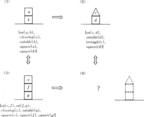
If each state is given by a finite set of ground literals as in Figure 8.10, a maximal partial match of 〈1〉 and 〈3〉 would be, for example,
Certainly there are other maximal partial matches. For example, both
and
are also maximal partial matches of 〈1〉 and 〈3〉.
Next, let us represent the state change from 〈1〉 to 〈2〉 by the transformation
where ![]() can generally be found using the following steps:
can generally be found using the following steps:
[1] Suppose (Q, (θ1, θ2)) is one of the maximal partial matches of (i) and (j). Then let ![]()
[3] Use for (8.21) the set of generalized literals obtained in [2].
For example, suppose we use the formula (8.20) as a maximal partial match. If we apply the substitution {a/X, b/Y} to 〈1〉 (including literals other than those in (8.20)), 〈1〉 is generalized to
Similarly, 2 is generalized to
by the substitution {c/X, d/Y). Therefore, (8.21) can be written as
If we apply the substitution given in (8.20) to parts other than the maximal partial match in 〈3〉, 〈3〉 is generalized to
If we replace the part in (8.24) that matches the left side of (8.23) with the right side of (8.23), we obtain
(8.25) represents state 〈4〉 that can be found based on learning by analogy. (8.25) can be illustrated as the broken lines in Figure 8.10.
Let us summarize the above description as a general algorithm. We assume that β1 β2 ∈ ß and τ1 ∈ T are given for the base domain B and the target domain T, and β1, β2, τ1 do not have common constant symbols.
Algorithm 8.3
[1] Find a maximal partial match m of β1 and τ1. (In the example, (8.22))
[2] Find a relation b12 of β1 and β2. (In the example, (8.23))
[3] Let ![]() be the generalization of τ1 using m. (In the example, (8.24))
be the generalization of τ1 using m. (In the example, (8.24))
[4] Find the element τ2 of T that corresponds to β2 using ![]() and b12. (In the example, (8.25))
and b12. (In the example, (8.25))
As we noted in (b), the important aspects of learning by analogy are that there is generally more than one maximal partial match for sets of literals and that a different analogy is found based on which maximal partial match is used. In the above example, a different analogy will be produced if we use another common part.
8.3 Nonmonotonic Logic and Learning
(a) Inference by nonmonotonic logic
Predicate logic is a just one kind of formal logic, but it sometimes cannot represent commonsense knowledge. Let us look at an example.
Let us represent the facts “tweety is a fish,” “a fish breathes through a gill,” “a mermaid is a fish,” “a mermaid does not breathe through a gill” by the set of axioms
where gills is a function symbol. Also, let us consider the set consisting only of modus ponens
as the set of inference rules. Now if we apply (8.26) to A, we can prove as a theorem
that is, the fact “tweety breathes through the gills.” However, suppose we later learn that “tweety is a mermaid.” If we add this to A and make the new set of axioms
A′= A U {mermaid (tweety)} (8.27) no longer holds and we have two inconsistent theorems:
(This implies that any well-formed formula is a logical consequence of A′.)
This contradiction occurs because a fact included in A′ has exceptions. In other words, the fact that a fish “usually” breathes through a gill but that a mermaid does not breathe through a gill even if it is a fish leads to a contradiction. The commonsense knowledge of human beings contains many such exceptions, and as the above example shows, a fact often stops being a fact when new knowledge is added. In this case, ![]() does not hold, where S(X) is the set of theorems that can be proved from a set of axioms X. This kind of logical inference is called inference by nonmonotonic logic.
does not hold, where S(X) is the set of theorems that can be proved from a set of axioms X. This kind of logical inference is called inference by nonmonotonic logic.
On the other hand, in ordinary predicate logic, ![]() always holds. In other words, if a theorem g can be proved from A by I, then g can also be proved by I from A ∪ {a} if a is a well-formed formula with the value of T. Logical inference with this monotonicity property is called inference by monotonic logic.
always holds. In other words, if a theorem g can be proved from A by I, then g can also be proved by I from A ∪ {a} if a is a well-formed formula with the value of T. Logical inference with this monotonicity property is called inference by monotonic logic.
Inference by nonmonotonic logic checks if a contradiction occurs with the already proved theorems every time a new fact is added to the set of axioms. If a contradiction occurred, the system needs to correct and generate a new set of theorems. This can be considered to be learning in the sense that existing knowledge changes due to new information.
(b) Default reasoning
First we will explain default reasoning, a kind of reasoning using nonmonotonic logic. Consider the following inference rule:
where P, Q, and R are n-place predicates, and X1,…, Xn are variable symbols. The above rule can be read as “if P(X1,…, Xn) is true and Q(X1,…, Xn) does not contradict other knowledge, then we assume that R(X1,…, Xn) is true.” Such a rule is generally called a default inference rule.
In the default inference rule, we call P the premise, Q the assumption, and R the hypothesis. Note that we call it an hypothesis rather than a theorem. This is because the truth value of well-formed formulas obtained so far can change when a new fact is introduced. The set of hypotheses that are obtained using a set of default inference rules is called the extension of default reasoning.
Suppose we have a set of axioms A, a set of inference rules of ordinary predicate logic I, and a set of default inference rules K. Then, generating from A a set of hypotheses that contain the well-formed formula g using I U K is called default reasoning.
In the example in (a), default reasoning means deriving
as a hypothesis using the default inference rule
In this example, respiration (X, gills (X)) is assumed not to contradict ∼ mermaid(X). Default inference rules often have the form where the assumption and hypothesis are identical, as in (8.28). This kind of default inference rule is generally called a normal default inference rule, and default reasoning based on a normal default inference rule is called reasoning based on normal default theory.
In default reasoning, the set of hypotheses to be found varies according to the order of application of default inference rules that generate hypotheses. For example, suppose “a substance is either a gas, a liquid, or a solid” is given as a fact. We represent this fact as the set of axioms
Furthermore, we define the inference rule “if a solid cannot be determined to be a gas (liquid or solid), assume that it is not a gas (liquid or solid)” as the following three default inference rules:
The set of hypotheses derived from A depends on which rule is applied first. For example,
As you can see from this example, default reasoning often generates more than one extension. Which extension to use cannot be determined purely by logical inference. It is determined by the purpose of the inference system and its interaction with the outside world.
The inference rules (i)-(iii) above are special cases of the rule
for an n-place predicate P(X1,…, Xn). (8.29) can be read “If the value of P(X1,…, Xn) cannot be determined to be T, we assume the value is F.” Logical inference on a computer sometimes assumes that ∼ P is proved if it cannot find a proof that P is T. This assumption is called the closed world assumption. We can use an inference rule like (8.29) to make the closed world assumption part of a default reasoning system.
Now we give an algorithm for default reasoning using normal default theory. Let A be a set of axioms, I a set of inference rules of predicate logic, K a set of normal default rules, and g the well-formed formula to be proved. We use f(k) and h(k) for the premise and the hypothesis of a rule k, respectively. For any k ∈ K, we define the subset L ⊆ K as
where ∧k∈L means the conjunction of all k in L. Furthermore, for A, g, and any L ⊆ K, we assume that f(L) and h(L) are represented as a set of clauses. Now, let us consider the following algorithm:
Algorithm 8.4
[1] Assume the value of h(K) is T and set D = A ∧ h(K) where A is regarded as a conjunction. Try to prove D ![]() g. We can do this by trying to prove D∪ {∼g} using the theorem proving algorithm based on the resolution principle.
g. We can do this by trying to prove D∪ {∼g} using the theorem proving algorithm based on the resolution principle.
[2] Let L be the subset of K, the set of default inference rules, whose hypothesis appears in the formulas used during the proof process of [1]. If L = ϕ, go to [4]. Otherwise, set N = N ∪ h(L) and go to [3].
[3] Do the proof A ∪ h(L) ![]() f(L). Go to [2].
f(L). Go to [2].
To find the set L in Algorithm 8.4 [2] we should keep the list of the default inference rules that were used in each theorem proving step. In the framework of first-order predicate logic, it is known that there does not exist a procedure that can determine the consistency of the set N as required in [4]. Therefore, in [4], we need to use some heuristic method to determine consistency.
Let us assume that, when [4] is executed in the above algorithm, g is found as a hypothesis from A, I, and K. The conditions that g is found as a hypothesis can be summarized as follows (this is another way of explaining the algorithm):
(ii) Subsets L1,…, Lm of K exist and ![]()
(iv) A ∪h (L1) ∪h(L2)∪…∪h(Lm) is satisfiable in the sense of first-order predicate logic.
We can rephrase the definition of default reasoning to be reasoning that satisfies (i)–(iv) above. Generating hypotheses from incomplete knowledge using default reasoning is an example of learning based on knowledge. We also need to remember that there may be more than one extension, that is, the set of hypotheses generated by default reasoning, depending on the order of using the default inference rules.
(c) Truth maintenance system (TMS)
The default reasoning described in (b) is a method of inference for generating hypotheses from incomplete knowledge. If we consider cases where new knowledge is incrementally added to the knowledge base, we sometimes need to change hypotheses that have already been added. For example, as in the example shown in (a), when the new fact
is added to the set of axioms

the hypothesis that had been obtained
no longer holds as a hypothesis.
Let us look at a truth maintenance system (we will call it a TMS) as an algorithm for changing hypotheses and maintaining the consistency of hypotheses. The TMS is related to default reasoning in the sense that both change hypotheses, but, as we show below, the former can be formalized as an algorithm that is seemingly unrelated to the latter. In order to avoid confusion, we will use the term belief rather than hypothesis below.
We consider an abstract object called belief that has two states, the In state and the Out state. Whether the state of a belief is In or Out depends on the states of other beliefs. More concretely, we say that the state of a belief b0 is In only when other beliefs b1,…, bi are all in the In state and bi+1,… bj are all in the Out state. If we interpret the In state as “believe” and the Out state as “do not believe,” the above can be read as “we believe b0 only when we believe b1,…, bi and do not believe bi+1,…, bj.”
When a new state of a belief is given, a TMS finds beliefs that can be justified by this state and, at the same time, computes all the state changes of other beliefs due to this justification.
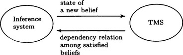
A TMS is a system that nonmonotonically keeps consistency of dependency relations among current beliefs: a new belief state is inferred by another inference system and sent to the TMS. The relation between a TMS and an inference system is shown in Figure 8.11.
Below we explain the representation of belief in a TMS and an algorithm for keeping the consistency of belief states. Note that an algorithm for a TMS is not related to what kind of knowledge representation is used for inference.
We represent a belief as a pair of a node and a justification:
A node name is the label for a belief. A justification is defined as a list with the meaning of (1) or (2) described below. Below 〈In list〉 and 〈Out list〉 are lists of node names, and (result) is a node name. A pair of 〈In list〉 and 〈Out list〉 described in a justification is called a support list.
(1) Support list justification: SL
The state of a node becomes In only when all the nodes included in its in list, 〈In list〉, are in the In state and all the nodes in its out list, 〈Out list〉, are in the Out state.
(2) Conditional proof justification: CP
The state of a node becomes In only when the states of the nodes in (result) become In under the condition that the states of all the nodes of 〈In list〉 are In and the states of all the nodes of 〈Out list〉 are Out.
means that, when N3 and N5 are in the In state and N4 and N7 are in the Out state, the node N1 is in the In state, and otherwise N1 is in the Out state. Also,
means that, if an inference system believes N6 under the condition that it believes N1 and N5 but does not believe N8, then N4 is in the In state, and otherwise N4 is in the Out state.
There are three kinds of support list justifications:
(i) When 〈In list〉 = 〈Out list〉 = 0. The state of the corresponding node is always In. A belief with this justification is called a premise.
(ii) When 〈In list〉 ± 0 and 〈Out list〉 = 0. A belief with this justification is monotonic in the sense that the state of the corresponding node does not change even when the nodes in the In state are added.
(iii) When 〈Out list〉 ± 0. For a belief with this justification, the state of the corresponding node can change as nodes in the In state are added. This belief is called an assumption.
A TMS holds beliefs and their states as defined above. Every time a new belief is input, it generates the states that do not contradict each other and outputs these states. In order to change the state of a belief, we can use some search algorithm. What we need to be careful of is that a nonmonotonic change can happen due to the fact that the state of a belief in a support list changes, or a new belief is entered into the support list and the corresponding justification can no longer be supported.
As an example, let us consider the set of beliefs shown in Figure 8.12. Figure 8.12 shows the states of beliefs about starting times and the type of transportation to use. These are input from an inference system for managing business trip schedules.
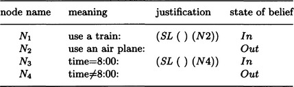
Suppose that the inference system found a contradiction between beliefs N1 and N3. (For example, it found that there is no train leaving at 8:00 due to a change in the train schedule.) The TMS adds the following two beliefs to the set of the original beliefs, and makes the states of both beliefs In:
where (8.31) can also be described as
Next, the TMS sets the state of (8.30) to Out and changes the state so that the states of the beliefs N1-N6 are consistent. The result is shown in Figure 8.13(a).
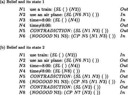
Now let us imagine that the inference system finds that N2 cannot be believed (for example, due to the information that dense fog has shut the airport). Then, the TMS generates the new beliefs with the In state,
and adds them to the set of beliefs in Figure 8.13(a). Here (8.33) can also be described as
Next, the TMS sets the state of (8.32) to Out and changes the state so that the states N1-N8 are consistent. The result is shown in Figure 8.13(b). The result shows that, since N1 and N4 are In and N2 and N3 are Out, we can keep the dependency relations among beliefs consistent if we use a train that leaves at any time other than 8:00.
(d) Assumption-based truth maintenance system (ATMS)
In the TMS described in (c), the only information associated with each node is its justification. Such justifications can only refer to local belief relations in order to maintain global consistency among beliefs. As a result, the computation is generally slow and the search for state change might get into a loop when using relations among nodes described only in the justifications. In order to eliminate these problems, it is sufficient to compute the set of hypotheses globally covering all the nodes from justifications. A system for computing the set of global hypotheses and, at the same time, maintaining dependency relations among beliefs is called an assumption-based truth maintenance system (ATMS hereafter).
Like a TMS, an ATMS receives information on relations among beliefs from an inference system and changes the dependency relations of beliefs so that they are consistent. However, unlike a TMS, it does not use the concept of the state of a belief. Instead, it always maintains and can change the whole set of hypotheses for keeping consistency among beliefs.
A node in an ATMS is represented as follows:
Here “the name of data” is information about a belief that is handled by the inference system and is given to the ATMS as data. Also, a justification is sent from the inference system in the form of
where a1,…,am (called the antecedents) are names of data, and b (called the consequent) is the name of a node of the ATMS. Furthermore, a special node called the contradiction node is defined in the ATMS, and if antecedents contradict each other, b becomes the contradiction node.
For any node, we call the set of names of data that can maintain consistency of beliefs a hypothesis. A hypothesis is computed from justifications using the algorithm given below. A set of possible hypotheses is called a label.
When a name of data and a justification are sent to the ATMS from the inference system, the label of the node that appears in the consequent of the justification is updated using the following algorithm:
Algorithm 8.5
[1] Using [1.1]-[1.4], repeat updating the label for a node given in the consequent for each of the justifications sent from the inference system. There, first update the labels of nodes that include the node whose label is changed in the antecedents of the justification.
[1.1] Obtain a label for ∨k ∧i Lik and compute Lik. Here Lik is the kth hypothesis at the node corresponding to the ith element in the antecedents of the justification.
[1.2] Of elements in the label obtained in [1.1], remove redundant or contradictory ones.
[1.3] When the new label is equal to the original label, stop. Otherwise, go to [1.4].
[1.4] When the node is the contradictory node, add the hypotheses to the database called NOGOOD, and remove all the contradictory hypotheses from the labels of all nodes.
As an example, let us consider the problem described in (c) (Figure 8.12). The node representations of the inference system and the ATMS for this problem are given in Figure 8.14(a) and (b).
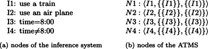
Suppose the information that nodes I1 and I2 and nodes I3 and I4 are contradictory is sent to the ATMS from the inference system. Then the ATMS generates the following NOGOOD database:
where the information from the inference system is given in the form of the justifications
Here ⊥ represents the contradictory node. As a result, of the 16 possible combinations of the hypotheses, there are nine consistent hypotheses that are circled in Figure 8.15. These nine hypotheses constitute the set of hypotheses at this time. Now, if the information that I1 and I3 are contradictory is sent to the ATMS using the justification
the hypothesis {I1,I3} becomes contradictory and is removed from the set of hypotheses. Also, {I1,I3} is added to the NOGOOD database. Furthermore, if the justification
is sent to the ATMS, the hypothesis {I2} and any hypothesis including I2 are removed from the set of hypotheses, and {I2} is added to the NOGOOD database.
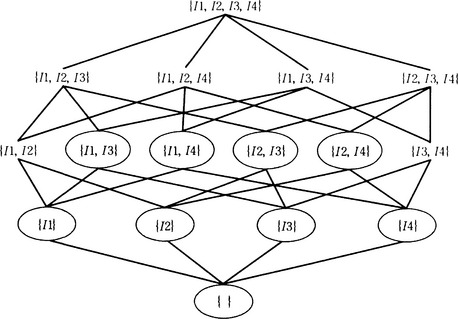
The set of hypotheses obtained so far is
This shows that the nodes I1 and I4 are not contradictory; in other words, using a train that leaves at any time other than 8:00 does not contradict the schedule.
As we can see from the above example, an ATMS uses an algorithm based on the updating of the set of hypotheses that are not contradictory or redundant, not the states of beliefs. This algorithm only requires removing hypotheses that cause contradiction from the set of hypotheses. It does not require local search of justifications as in a TMS.
Summary
In this chapter, we described algorithms for learning by generalization based on logical inference and methods of truth maintenance of hypotheses based on nonmonotonic logic.
8.1. Explanation-based generalization is a method of finding an explanation for how an instance is a positive instance of a given concept using the concept and one positive instance of it and generalizing a proof tree that is found by theorem proving.
8.2. If we restrict the representation to Horn clause logic, we can write a program for explanation-based generalization in Prolog.
8.3. Learning by analogy is done by finding a maximal partial match for two sets of literals.
8.4. Nonmonotonic logic can be used for learning based on logical inference. Default reasoning using default inference rules is one popular example.
8.5. A truth maintenance system (TMS) is a system for generating a set of new hypotheses by checking local consistency of existing hypotheses, when new facts are incrementally added to the knowledge base.
8.6. An assumption-based truth maintenance system (ATMS) is a system that generates a set of new hypotheses by checking the global consistency of the set of hypotheses.
Keywords
explanation-based generalization, goal concept, domain theory, operationality criterion, Horn clause logic, unification, analogy, learning by analogy, partial match, maximal partial match, nonmonotonic logic, default reasoning, truth maintenance system, belief, support list, justification, assumption-based truth maintenance system, set of hypotheses
Exercises
8.1. In the example of explanation-based generalization described in Section 8.1(b), when the positive instance is
and the domain theory is

what result do we get if we use a Prolog program in Figure 8.6? Find a proof tree and a generalized proof tree like the ones shown in Figure 8.8 and a sufficiency condition such as formula (8.8). How is the sufficiency condition generalized compared to the original positive instance?
8.2. Suppose we have the finite sets of ground literals
(i) Find a maximal partial match, m, of β1 and τ1.
(ii) Express the state change from β1 to β2 in the form of a transformation as in (8.21).
(iii) Find ![]() , a generalization of τ1, by applying the substitution in m to τ1.
, a generalization of τ1, by applying the substitution in m to τ1.
(iv) Do the transformation of (ii) on ![]() and let the result be τ2. (Then τ2 is the result of learning by analogy that uses {β1, β2} as the base domain and {τ1} as the target domain.)
and let the result be τ2. (Then τ2 is the result of learning by analogy that uses {β1, β2} as the base domain and {τ1} as the target domain.)
8.4. Suppose we are given the facts that a swallow, a sparrow, a robin, and a hawk are birds. What inference rule do we need to make logical inference that the only birds are (or equivalently birds are circumscribed to be) a swallow, a sparrow, a robin, and a hawk? Generalizing the obtained rule, describe an inference rule that says “if an object x has a property p, the objects that have property p are circumscribed to be x.” This generalized rule is a well-formed formula in second-order predicate logic. (Logical inference using this kind of inference rule is called circumscription. Circumscription is known to be a method of nonmonotonic reasoning.)