Learning Procedures
In this chapter we will explain methods of learning procedures for transforming information, such as operators in problem solving, production rules, and computer programs. Representations of these procedures not only are more complex than those of concepts but also have a deep relation to inference methods. Therefore, learning procedures require different methods than learning concepts. In this chapter we will learn basic methods for learning procedures by explaining several popular algorithms.
7.1 Learning Operators in Problem Solving
A solution to a problem in problem solving can be represented as a sequence of operators for moving from the initial state to the goal state. By solving one problem, generating a sequence of operators necessary in solving a problem, and generalizing such a sequence, we have the possibility of solving other problems. Learning, in this sense, is a typical example of learning procedures and is called learning operators in problem solving. We will explain methods of operator learning in problem solving in this section.
(a) Problem solving by theorem proving
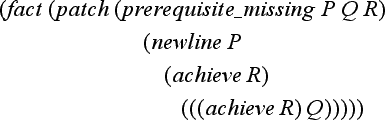
Suppose we have a problem P = 〈S, O, F, so, sd〉. First, we will describe a method of finding a solution for P using the technique of theorem proving. We represent a state s ∈ S by the conjunction of predicates, or equivalently a set of predicates. Also, we represent an operator o ∈ O by the triple 〈p, d, a〉 of preconditions p, a delete list d, and an add list a, where p, d, and a are each a set of predicates. Moving from a state s to another state s′ by applying an operator o is equivalent to generating s′ = s ∪ aη − dη under the condition that the constraint s → pη holds for some substitution η. If we consider the initial state so as a set of axioms and the goal state sd as a set of theorems, we can say that we have solved P when we have proved all the elements of sd, starting from so.
Let us represent by s ![]() t the fact that all the elements of a set of predicates t can be proved from a set of predicates. Given that we can use the method described in Chapter 3 as an algorithm for theorem proving, we can give an algorithm for solving a problem P using theorem proving as follows:
t the fact that all the elements of a set of predicates t can be proved from a set of predicates. Given that we can use the method described in Chapter 3 as an algorithm for theorem proving, we can give an algorithm for solving a problem P using theorem proving as follows:
Algorithm 7.1
(problem solving based on theorem proving)
[2] Try to solve s0 ![]() g. If it is proved, then stop. We take the sequence of operators applied so far as a solution to the problem. If it is not proved, let g be the set of predicates necessary for the proof and go to [3].
g. If it is proved, then stop. We take the sequence of operators applied so far as a solution to the problem. If it is not proved, let g be the set of predicates necessary for the proof and go to [3].
[3] Pick an operator where the add list and g match. If we find such an operator, let g be its preconditions and go to [2]. Otherwise, stop. A solution to the problem does not exist.
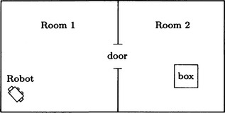
Let us consider the problem, P, of how a robot, robot1, in a room, room1, can bring the box box1 from another room, room2, to the room, room1. The arrangement of the rooms is shown in Figure 7.1.
We assume that the initial state of P, so, the goal state, sd, and the three available operators represented as a triple are given as follows:
| initial state so: | in(robot1, room1) |
| in(box1, room2) | |
| connect (door1, room1, room2) | |
| connect(door1, room2, room1) | |
| robot(robot1) | |
| box(box1) | |
| door(door1) | |
| room(room1) | |
| room(room2) | |
| goal state sd: | in(robot1, Y) |
| in(box1, room1) | |
| connect(D, X, Y) | |
| connect(D, Y, X) | |
| robot(robot1) | |
| box (box1) | |
| door(door1) | |
| room(room1) | |
| room(room2) |
The rule walkto(R, W, X, Y) means to delete the condition that R is in X and add the condition that R is in Y, provided that a robot R is in X and that X and Y are connected by W. This rule can be read as “R moves from X to Y through W.” The rule carryto(R, B, W, X, Y) similarly can be read as “if R is in the same room as the box B, R moves to the connecting room carrying B.”
To prove the theorem, we need to prove that all the predicates in sd are true. Let us describe only the proof of in(box1, room1) to save space. For simplicity, we suppose sd = {in(box1, room1)}.
[1] Set g = sd = {in(box1, room1)}.
[2] Since s0 ![]() g cannot be proven directly, go to [3].
g cannot be proven directly, go to [3].
[3] Of all the operators, the add list a2 of carryto matches g by the substitution θ1 = {box1/B, room1/Y}. So, set g = p2θ1 = {in(R, X), in(box1, X), connect(W, X, room1), robot(R), box(box1)}.
[2] Try to prove so ![]() g. The process of proof by resolution is shown in Figure 7.2(a). As shown in Figure 7.2(a), in order to prove s0
g. The process of proof by resolution is shown in Figure 7.2(a). As shown in Figure 7.2(a), in order to prove s0 ![]() g, we only need to prove in(robot1, room2) in order to prove s0
g, we only need to prove in(robot1, room2) in order to prove s0 ![]() g. So, set
g. So, set
[3] Of all the operators, the add list a1 of walkto matches g by the substitution θ2 = {robot1/R, room2/Y}. So, set
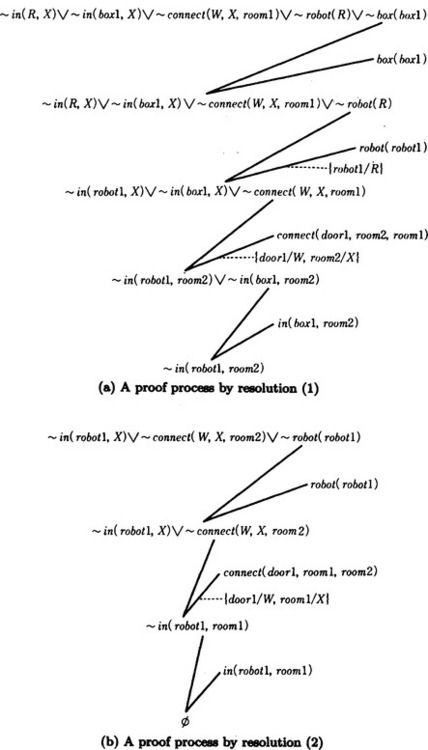
[2] so ![]() g can be proven. The proof is shown in Figure 7.2(b). As a result, a solution to the problem can be represented as the sequence of operators:
g can be proven. The proof is shown in Figure 7.2(b). As a result, a solution to the problem can be represented as the sequence of operators:
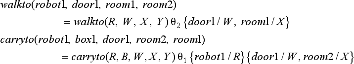
In other words, if we apply these rules to the initial state in order, we obtain the goal state. The above solution can be interpreted as “robot1 moves from room1 to room2 and goes back to room1 with the box box1.”
(b) Generalization of operators
A sequence of the operators obtained by theorem proving exemplified in (a) can be regarded as a procedure for transferring a given initial state to a goal state. However, such a procedure can be used only in a specific problem and cannot be used in different problems even with as simple a change as renaming a room. For example, if we change room1 and room2 to other symbols, we cannot be sure that the original procedure is usable.
One method of removing this restriction is to generalize the procedure that was found so that it can be used in other problems. Below, we describe a method for generalizing a sequence of operators obtained by solving the problem P.
First, we represent the sequence of operators we found by solving the problem P in a triangular table. A triangular table represents states of the problem and applicable operators using the lower left triangular part (including the diagonal line) of a square matrix of size n + 1, where n is the length of the sequence. Each row of a triangular table represents a state transition in order from the top. To the right of the row we put the operator that was used in the state transition. The leftmost end of the row contains the set of the predicates that were included in the initial state and used as preconditions when applying the operator. The predicates that are added to the preconditions by the operator in the i − 1th row are written in the intersection of the ith column and ith row (2 ≤ i ≤ n + 1). Similarly, the predicates that were not deleted from the preconditions by the operator in the j − 1th row are written in the ith column and jth row (i < j ≤ n + 1). For example, the sequence of operators obtained in the example described in (a) can be represented as the triangular table shown in Figure 7.3.

Next, we generalize the sequence of operators represented by the triangular table in the following steps:
Algorithm 7.2
(generalizing a sequence of operators)
[1] Replace constant symbols with variable symbols in the predicates that are in the leftmost column of the triangular table (![]() ,
, ![]() ,
, ![]() , in Figure 7.3), where if the same constant symbol is used in two or more places, replace each of them with a different variable.
, in Figure 7.3), where if the same constant symbol is used in two or more places, replace each of them with a different variable.
[2] Replace the arguments of each operator with different variable symbols. Let θ be the substitution for the replacements.
[3] Using θ, replace the arguments of the add list with variable symbols.
[4] Using the rules that are generalized in [1]–[3], repeat the proof of the original problem once more. This can be done by using the fact that the predicates in the ith row of the triangular table are used to prove the preconditions of the operator that will be used at the ith step. In this second proof, we use the predicates in the same way as in the original proof. The reason for doing the proof once more is to prevent inconsistent substitutions for the variables in the predicates.
[5] The operators that are found in this way are possibly overgeneralized. To prevent this, redo the substitution of variables by applying the sequence of new operators to the original problem.
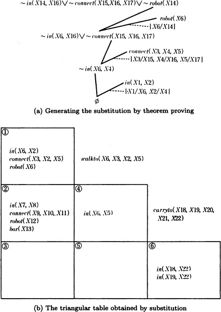
As an example, let us find a sequence of generalized operators from the triangular table shown in Figure 7.3. First, if we apply [1]–[3] to the triangular table in Figure 7.3, we obtain the generalized triangular table shown in Figure 7.4.
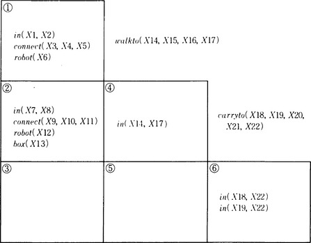
Next, as stated in [4], redo the proof using the table in Figure 7.4. This proof proceeds as follows:
(1) Prove the preconditions of walkto (X14, X15, X16, X17) using Figure 7.4 ![]() . (Figure 7.5(a)). Apply the substitution obtained by this to the triangular table of Figure 7.4 to obtain a new triangular table (Figure 7.5(b)).
. (Figure 7.5(a)). Apply the substitution obtained by this to the triangular table of Figure 7.4 to obtain a new triangular table (Figure 7.5(b)).
(2) Prove the preconditions of carryto (X18, X19, X20, X21, X22) using Figure 7.5(b) ![]() ,
, ![]() (Figure 7.6(a)). Apply the substitution obtained by this to Figure 7.5(b) to obtain a new triangular table (Figure 7.6(b)).
(Figure 7.6(a)). Apply the substitution obtained by this to Figure 7.5(b) to obtain a new triangular table (Figure 7.6(b)).

From Figure 7.6(b), we learn that the sequence of generated operators
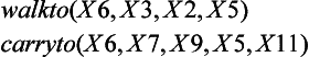
is a generalization of the one shown in Figure 7.3. We can interpret the sequence of generalized operators as: “The robot X6 moves from the room X2 to the room X5 through door X3. Next, X6 carries the box X7 and moves from the room X5 to the room X11 through the door X9.” Since the same symbol does not have to be substituted for X2 and X11, the robot can move to a room different from the one where it was originally located.
As you can see, the goal state obtained by the sequence of generalized operators can be different from the goal state of the original problem. In the above example, the difference occurs because the variable, X22, in ![]() is different from the variable, X2, in
is different from the variable, X2, in ![]() in the triangular table of Figure 7.4. One method of preventing this overgeneralization is to apply the sequence of generated operators in Figure 7.6(b) to the original problem and redo the substitution of the variables, as described in [5] of the algorithm. Doing that, we see that we should do the substitution {X2/X11} in carryto. We can obtain a sequence of new operators from this substitution:
in the triangular table of Figure 7.4. One method of preventing this overgeneralization is to apply the sequence of generated operators in Figure 7.6(b) to the original problem and redo the substitution of the variables, as described in [5] of the algorithm. Doing that, we see that we should do the substitution {X2/X11} in carryto. We can obtain a sequence of new operators from this substitution:
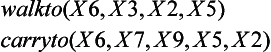
If we apply this sequence of operators to the initial state of the original problem, the robot X6 goes from the room X2 to the room X5, takes the box X7, and goes back to the original room X2 with the box, where the names of the doors between X2 and X5 are represented by the two variables X3 and X9. This means that the robot does not have to go though the same door between the two rooms as it goes back and forth. In this sense, the sequence of operators obtained above is generalized not only in the sense that constant symbols are replaced by variable symbols but also as a method of problem solving.
This algorithm is heuristic and the generated sequence of operators can be redundant or provide inconsistent solutions. In such cases, we need to modify the operators to eliminate redundancy or resolve inconsistency by using some heuristics.
Also, in this technique one state transition is done by one operator, but sometimes more than one consecutive state transition could be done by one operator. Such an operator is called a macro-operator. A macro-operator can be generated by learning. In the above example, a generalized macro-operator can be synthesized from the operators walkto and carryto.
7.2 Learning Rules
In this section, we will describe a method for learning procedures represented as production rules. Production rules can be learned by giving a production system the capability of generating a new rule by itself and adding it to the set of rules. Below, we will describe general methods for learning and generalizing rules, and later we will describe examples of learning rules.
(a) Methods of rule learning
A new production rule can be learned by giving to the action side of a rule in a production system the capability of generating new rules and the action of adding these new rules to the original set of rules. A production system with the capability of generating rules is called an adaptive production system. Now we will describe methods of generating new rules used in adaptive production systems. Here by a production system we mean a production system with ordered rules. The following methods can be used in combination with each other.
(1) Independent addition of rules
This method generates a new rule all at once in the action side of one rule and adds it to the original set of rules. This method of learning is called the independent addition of rules, because such rules are independent of the original ones. For example, let us consider the following set of rules:
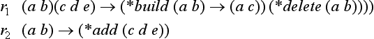
Here *build is a function for adding its value to the top of the set of original rules. *delete and *add are functions that delete the value of its argument from working memory and add the value of its argument to working memory, respectively.
We assume that *add can be omitted. In other words, when the action side of a rule has a list without a function name as its first element, we assume that such a list has *add as its first element. Also, we represent working memory as a list of lists. If we assume the initial state of working memory is ((a b)), these rules are executed as shown in Figure 7.7. In the execution of *build, the name of the rule to be generated is automatically created, and the list 〈〈name of the rule〉 built) is added to working memory. Also, in the above example, the rule does not include any variables, but a similar method can be used when the rule includes variables.
(2) Dependent addition of rules
This method first generates components of the rule to be learned (each condition and action) separately and maintains them with a marker in working memory. When all the components are ready, it makes a new rule and adds it to the original set of rules. This method is called dependent addition in a sense that the rule learning is dependent on several rules. Section 7.2(c) will describe an example of learning by the dependent addition of rules.
(3) Generalization of rules
As in generalization of concepts, there are several methods for generalizing rules.
(i) Replacing constants with variables
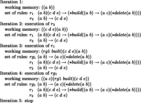
This method generalizes a rule by replacing constants by variables within one rule. An example of this method is shown in Figure 7.8. *generalize in Figure 7.8 is the function that, for the rule whose name is given in its first argument, generalizes constants bound to its second argument to new variables. When *generalize is executed, constants are replaced by variables in a specific rule and the rule is added to the top of the original set of rules.
(ii) Replacing constants with functions
This method generalizes a rule by replacing constants with functions within one rule. For example, it can generate the new rule
from the rule
by replacing a and b with $x and (next $x), respectively, and adding the new rule to the top of the original set of rules.
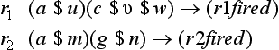
(iii) Generalizing from two rules
This method generates a new rule that is executable whenever either one of two rules can be executed and adds it to the top of the original set of rules. This is done by making the set of conditions for the new rule C1 ∩ C2 or its subset (ignoring differences in the names of variables) when the original sets of conditions for the two rules are C1 and C2, respectively. For example, we generate
from
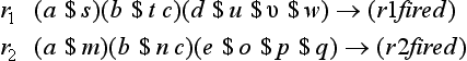
where rg1 is a generalization of r1 and r2 in the sense that rg1 is executed when either r1 or r2 is executed. However, since this method is likely to result in overgeneralization, it usually selects a most specific rule among the generalized rules, as in an MSC generalization for concept learning.
is a generalized rule for r1 and r2, but rg1 is a more specific rule than rg2. Actually, in this example, rg1 is the most specific rule, and rg1, not rg2, would be generated.
(4) Specialization of rules
In addition to generalization, we can generate new rules by specializing an already existing rule.
(i) Replacing variables with constants
One method is to make a more specific rule by replacing variables with constants within one rule and adding the new rule to the original set of rules.
(ii) Replacing functions with constants
Another method is to make a more specific rule by replacing functions with constants within one rule and adding the new rule to the original set of rules.
(iii) Specializing one rule from two rules
Given two rules r1 and r2, we make a new rule rs1. This method constructs rs1 so that r1 and r2 are both executable whenever rs1 is executable. The newly made rule is added to the top of the original set of rules. For example, we can generate
from
Here rs1 is a specialization of r1 and r2.
As in generalization, overspecialization can happen when specializing a pair of rules. For example,
is a specialization of r1 and r2, but it is a more specific rule than rs1. Usually we select a maximally general specialization as the new rule.
(5) Composing rules
This method generates a new rule whose execution has the same result as the consecutive execution of two existing rules and adds the new rule to the top of the original set of rules. For example, suppose A and C are the sets of conditions and B and D are the sets of actions for each rule. If we know that two rules

are always executed in this order, we can generate the new rule
and add it to the top of the original set of rules. After rc1 is added to the set of rules, rc1 is executed whenever r1 and r2 would be executed consecutively. As a result, the state of working memory would be the same as if r1 and r2 had been executed.
Composition of rules is a learning method similar to generating macro-operators, described in Section 7.1.
(b) Learning by generalizing rules
Here we will explain learning by generalization of rules in detail. We will assume that we have a production system that satisfies the following conditions:
(1) The only actions allowed by a rule are storing and deleting lists in working memory.
(3) In any rule, lists that are deleted by executing the action side of the rule appear explicitly in the condition side of the rule.
For a production system satisfying (1)–(3), each rule can be represented as
where a2 is a set of conditions, and b1 and b2 are actions for deleting lists from and adding lists to working memory, respectively. Here we are assuming that all the actions for deleting lists are executed before the actions for adding lists.
If we let c be the set of lists that are included in a2 but not included in b2 and let a1 = a2 − c, we can write the rule (I) as
The set c is called the context. We use σ to denote the content of working memory. A necessary condition for [c]a1 → b1 to be executable for σ is that there exists a substitution θ satisfying
In this case if [c]a1 → b2 is executed for σ, the content of working memory is replaced by ![]() .
.
Below we define generalization of rules, assuming that all of the rules have the form [c]a1 → b1.
Definition 1
(generalization) If, for the rules r1 and r2,
for any working memory σ and σ′, we call r1 a generalization of r2, where ![]() denotes transforming the content of working memory from μ to μ′ by executing the rule r. Let r1 ≤ r2 denote that r1 is a generalization of r2.
denotes transforming the content of working memory from μ to μ′ by executing the rule r. Let r1 ≤ r2 denote that r1 is a generalization of r2.
Definition 2
(strong generalization) Assume r1 ≤ r2 for some rules r1 and r2. If there is no substitution θ that makes r1 = r2θ, we call r1 a strong generalization of r2 and write r1 < r2.
In generalizing a rule, the following holds: suppose that for two rules ![]() and
and ![]() , there is a substitution θ such that
, there is a substitution θ such that ![]() and
and ![]() . In this case, a necessary condition for
. In this case, a necessary condition for ![]() is that a substitution ξ exists for which
is that a substitution ξ exists for which ![]() .
.
Next, let us define the following for creating a rule by generalizing two rules:
Definition 3
(common generalization) For two rules r1 and r2, we call a rule r3 such that r3 ≤ r1 and r3 ≤ r2 a common generalization of r1 and r2.
There may be many common generalizations of two rules. Just as in the case of MSC generalizations in learning concepts, it is generally better to choose a common generalization that is “close” to the original rules (here, r1 and r2). To do that, we introduce the following definition:
Definition 4
(maximal common generalization) When rules r1, r2, and r3 satisfy the following condition, we call r3 a maximal common generalization of r1 and r2: there does not exist a rule r′3 such that (1) r3 ≤ r1 and r3 ≤ r2 and (2) r3 ≤ r′3, ≤ r1, and r′3 ≤ r2.
For example, let us look at the following four rules:
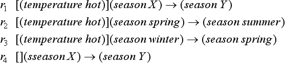
Here r1 ≤ r2, r1 ≤ r3, r4 ≤ r2, and r4 ≤ r3. Therefore, r1 and r4 are common generalizations of r2 and r3, respectively. However, since r4 ≤ r1, r4 is not a maximal common generalization of r2 and r3. On the other hand, r1 is a maximal common generalization of r2 and r3. Note that a maximal common generalization is not always unique even if we identify different ways of making substitutions.
Now, when a rule r1 is a maximal common generalization of r2 and r3, there exist substitutions θa and θb such that
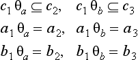
because of the statements given below Definition 2. If |·| is the number of elements included in a finite set · and |a1| ≠ |a3| or |b2| ≠ |b3| for r2 and r3, then a maximal common generalization of r2 and r3 cannot exist. As we can see from this example, in obtaining a maximal common generalization for two rules, the condition that |a2| ≠ |a3| or |b2| ≠ |b3| for the number of the elements of a2, a3, b2, b3 in these rules becomes an easily identifiable termination condition.
A maximal common generalization of two rules, if it exists, can be obtained by finding the substitutions θa, θb by an appropriate pattern matching algorithm. Also, a set of maximal common generalizations for three or more rules can be obtained by repeating the operation of obtaining a maximal common generalization for two rules.
(c) Learning by rule addition
Rule addition is one of the simplest learning methods for production systems, and because of its simplicity, it is widely applicable. Here we will describe learning by dependent addition of rules.
Let us consider a method of learning called paired-associate learning. This is a simple method of associative memory to remember pairs of information and recall one of a pair of information when the other is presented. For example, suppose we want to remember pairs of symbol strings that are made of three letters such as (rej qin), (ruk nac), …. Remembering such pairs and recalling the three letters on the right side of a pair when the three letters on the left side of the pair are given can be easily done by searching a table of these pairs. Here, let us consider the case of answering with three letters from the right side when only one or two letters from the left side are given. For a learning system that is able to search using only partial information, we need to index the symbol strings to be remembered. Below, we describe a method using dependent addition of rules as a learning algorithm for doing indexing automatically.
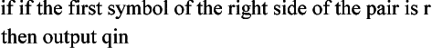
First, let us look at the case of answering qin whenever the first letter of the left side of a pair is r. This procedure can be said to be learned if the learning system generates the rule by itself
and adds this rule to the original set of rules. In order to do this learning, let us consider the program for a production system that uses the nine rules p1–p9 shown in Figure 7.9. Here the rules are in the order p1 through p9 and the program is an ordered production system. Also, we assume that not only lists but also predicates can be given in the condition side of a rule. A list condition is satisfied when it matches working memory. A predicate condition is satisfied when its value is T.
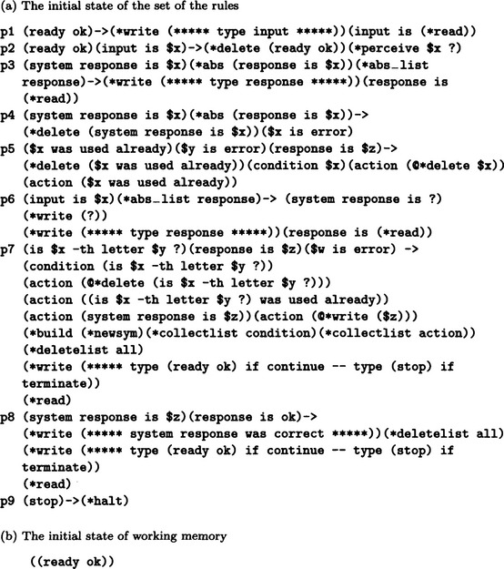
First, we will explain the predicates and functions in Figure 7.9. *abs is the predicate that takes T if and only if the list in its argument does not match working memory. *abs–list is the predicate that takes a symbol as an argument and is T if and only if no list in working memory contains that symbol as its first element. *delete is a function that deletes lists from the working memory. *deletelist is a function for clearing working memory when its argument is the atom all. *collectlist is a function for collecting all the lists in working memory that have its argument as their first element, making a new list of these lists, and adding it to working memory. *read and *write are functions for input and output, respectively. *newsym is a function that generates a new atom.
*perceive is a function for dividing a symbol string that appears as its first argument into its constituent symbols, generating three lists (i (ith symbol) (the second argument of perceive〉) (i = 1, 2, 3), and adding the lists to working memory in the order i = 2, 3, 1. Finally, *build is a function that generates a rule, which has the rule’s name as its first argument, conditions, as elements of the second argument, and adds the rule to the original set of rules. For an atom that contains the character @ in the program, @ will be deleted when the atom is stored in working memory.
Next, we will explain each rule in Figure 7.9. First, p1 is a rule for reading the information in the left side of each pair. p2 is a rule for dividing the string read in p1 into separate symbols, p3 is a rule for reading the information in the right side of each pair. p4 is a rule that is activated when the response from the system is not the correct response. p5 is a rule for collecting data in order to generate a new rule. p6 is a rule for reading the first response. p7 is a rule for generating a new rule. p8 is a rule that is activated when the response from the system is correct. p9 is a rule for terminating the execution.
Furthermore we assume that the initial state of working memory consists of one list, (ready ok), as is shown in Figure 7.9.
Figure 7.10 shows the result of executing the program. When the first information rej is input, p1 and p2 are executed consecutively, then p6 is executed, and the information qin that forms a pair with rej is input. After the execution of p4, a new rule g0184 is generated by p7. g0184 can be interpreted as
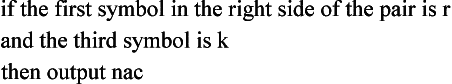
Next, ruk, the left side of a second pair, is input by p1. Then, right after p2, g0184 is executed, and qin is returned as the answer. This is a wrong answer due to the accidental fact that the first symbol of ruk is r. So, nac is now read as the right side of ruk by p3. Through p4 and p5, a new rule g0186 is created by p7. g0186 can be interpreted as
As a result, after the rules g0814 and g0186 are generated and added to the set of rules, the correct answers, gin and nac, are returned for rej and ruk, respectively. The last half of Figure 7.10 shows such answers.
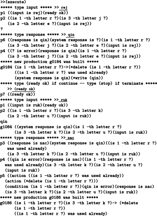
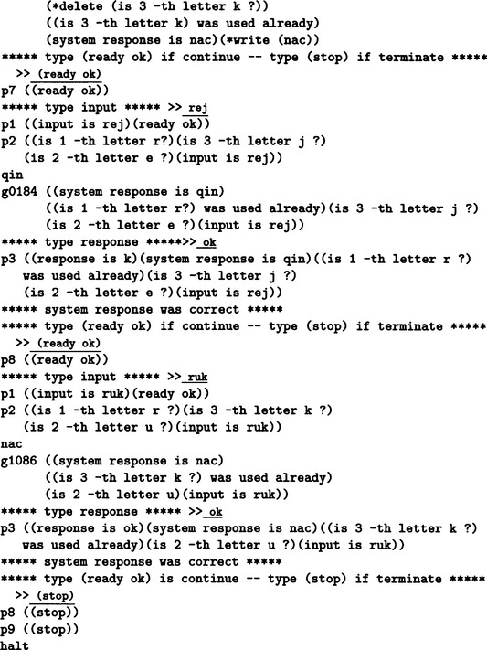
Figure 7.10 Execution of learning for the production system shown in Figure 7.9 (underlined words are input).
7.3 Learning Programs
In this section we describe learning procedures that are represented in the form of programs. Examples of learning complicated procedures include constructing algebraic functions and Lisp functions or constructing computer programs from input-output examples. Currently it is very difficult for a system to learn automatically complicated functions or programs. Some people are doing research on systems that enable a user to make a program by interacting with the computer. However, when a program is complicated, the system that supports this interactive programming requires a lot of knowledge about programs and programming. Thus how to represent this information in a computer becomes an important problem.
In this section, we will concentrate on a system for learning problem solving procedures in the form of programs.
(a) Learning a problem solving program based on knowledge
Consider problem solving in the world of blocks shown in Figure 7.11. The problem is to find a sequence of operators that transforms the initial state so to the goal state sd. Let us first represent the states in the form of lists.
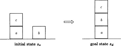

We call the set sd−so the goal and represent it using the function:
We can think of this problem as one of finding a procedure for deriving the goal from the initial state, so (under the condition that sd ∩ so is included in the goal state). To solve the problem, we need only search for an appropriate procedure leading to the goal from so using a knowledge base about such procedures. However, there is no guarantee of finding such a procedure directly. So, in case the procedure cannot be found, we should search a procedure leading to a similar goal.
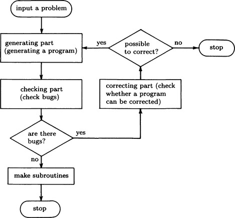
Next, when a problem cannot be solved by the procedure we found during the search, we need to find the cause of the failure, in other words, a bug in the program. We then examine the type of bug and search for a procedure for removing this type of bug using the knowledge base. Then we correct the procedure for reaching the goal using the procedure obtained for removing bugs. If we could solve the problem using the corrected procedure, we make the procedure a subroutine and add it to the knowledge base.
This method is summarized in Figure 7.12
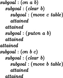
One common kind of bug is in the order of satisfying subgoals. For example, in the problem of Figure 7.11, suppose there are two subgoals, (on b a) and (on c b), and we reach (on c b) first and then try to reach (on b a). If we move c that is on b onto a, we return to the initial state that causes a loop in the state transition. This is due to the fact that each subgoal is regarded as an independent goal. In order to avoid this, there are search methods that change the order of subgoals and a method called goal regression that tests whether the result of attaining a subgoal contradicts some other subgoals.
(b) An example of learning
Here we describe how a system learns a problem solving program based on the method described in (a), using the example shown in Figure 7.13. In this example, appropriate procedures are immediately obtained from the knowledge base; however, in more complex cases, we generally need to do backtracking if the search finds inappropriate procedures.
(1) Executing the generation part
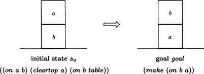
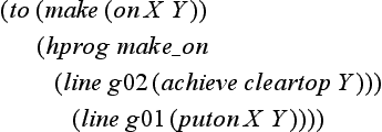
Suppose we found the following function in the knowledge base that is a procedure for reaching the goal, (make (on b a)), in the problem of Figure 7.13:
where hprog is a function that explains what the function to does, gives make_on as the name of the subroutine to, and shows that the function (puton X Y) is defined on line g01.
Also, when this function is in the knowledge base, the lists
are also stored in the knowledge base. The program (7.2) indicates that the goal of the subroutine shown in (7.1), make_on, is (make (on X Y)). The program (7.3) indicates that the purpose of g01, the statement of the subroutine make_on, is to (make (on X Y)), Now, suppose that a program like (7.1) was found in the generation part of Figure 7.12.
(2) Execution of the checking part
The checking part of Figure 7.12 executes the program (7.1) using the substitution {b/X, a/Y}. However, in the example in Figure 7.13, (7.1) cannot be applied to the initial state, so (7.1) is sent to the correcting part of Figure 7.12.
(3) Execution of the correction part
The correction part discovers bugs and determines their types. Suppose the reason why the program (7.1) cannot be executed on the initial state is that the function puton inside (7.1) does not work since (on a b) cannot be found in the initial state. This bug can be described as
Next, suppose we search the knowledge base for the conditions that will allow us to remove the bug in (7.4) and we find
The program (7.5) says that, if V is a function for moving a block W, we cannot execute V unless there is nothing on W. Since the program (7.6) can be substituted into (7.5) by the substitution {(puton X Y)/V, X/W}, we only need to check whether (cleartop X) is true in order to remove the bugs.
is true for the substitution {b/X}. Since (7.7) is not true for the initial state, the type of the bug can be determined to be
Next, we need to correct the original program (7.1) to eliminate bugs of type (7.8). Suppose we found the following knowledge in the knowledge base as a procedure for correcting a program:
Program (7.9) tells us how to insert a new statement right before the statement Q where the bug is found in the original program P so that the new program satisfies the unsatisfied condition R.
(c) Learning by detecting and deleting bugs
The system we explained in (b) is an example of a system for learning a new program by detecting and deleting bugs during problem solving. As you can see from this example, the learning of complicated programs needs to have a large amount of information in the knowledge base. Also, we assumed in this example that a bug can be easily detected, but it is often not easy to identify the bug that causes a program error. Furthermore, even if the system generates a program that has no bugs, we do not know much about what kinds of problems this new program will solve. What we explained in this section is a simple example of learning based on knowledge. When we apply these techniques to larger problems, we need to solve many supplementary problems.
Summary
In this chapter we learned methods that can be used to learn procedures that are used in inference and problem solving.
7.1. If a sequence of operators for solving a problem can be found using a theorem proving algorithm, a system can learn a sequence of operators for solving more general problems by generalizing the proof process.
7.2. A production system can learn production rules in various ways.
7.3. We can construct a system that learns problem solving procedures in the form of a program.
Exercises
7.1. Suppose in the problem solving of the robot (Figure 7.1), which is described in Section 7.1(a), the goal state sd is “the box box1 is in room room1 and the robot robot1 is in room room2.” Find a sequence of operators for reaching sd.
7.2. Make a triangular table using the answer of Exercise 7.1, and generalize it and find a sequence of generalized operators.
7.3. Write a program for an adaptive production system that performs dependent addition of rules described in Section 7.2(a)(2), where the system is assumed to be an ordered production system. You can use any programming language.
7.4. In the problem in Figure 7.14, suppose the goal is given as
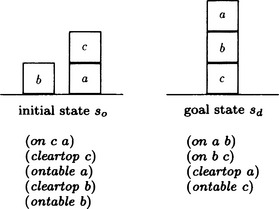
Figure 7.14
Then a loop occurs if subgoals are attained as follows: