
Chapter 41. Parallelization of Katsevich CT Image Reconstruction Algorithm on Generic Multi-Core Processors and GPGPU
Abderrahim Benquassmi, Eric Fontaine and Hsien-Hsin S. Lee
41.1. Introduction, Problem, and Context
Medical imaging is one of the most computationally demanding applications. Radiologists and researchers in related areas such as image processing, high-performance computing, 3-D graphics, and so on, have studied this subject extensively by using different computing facilities, including clusters, multicore processors, and more recently, general-purpose graphics processing units (GPGPU) to accelerate various 3-D medical image reconstruction algorithms. Because of the nature of these algorithms and the cost-performance consideration, recent works have been concentrating more on how to parallelize these algorithms using the emerging, high-throughput GPGPUs. An interesting medical imaging modality widely used in clinical diagnosis and medical research is computed tomography (CT). CT scanners have been the focus of studies attempting to accelerate the reconstruction of their acquired images. CT scanners are classified into parallel fan-beam and cone-beam devices. The cone-beam type can be labeled as circular or helical, based on the path its X-ray source traces. In circular CT scanners, the X-ray source completes one circular scan, then the platform holding the patient is moved forward by a certain amount, and a new circular is performed, and so on. The length that the table was moved determines the CT scanner slice thickness. In the case of helical scanners, the X-ray source keeps rotating while the platform holding the patient continuously slides inside the scanner's gantry. The movement of the table is a linear function of the X-ray source rotation angle. In the Cartesian frame reference attached to the table, the X-ray source traces a helical path whose axis is parallel to the scanner's table, as depicted in
Figure 41.1
. The helical type of scanner is preferred in medical imaging, but it comes with the cost of a complicated reconstruction algorithm. The source emits X-ray beams that traverse the patient's body and get attenuated by a factor that depends on the medium density. The attenuation factors are recorded as the acquired data from the detectors. These attenuations are used to infer the density of the different tissues constituting the travel medium.
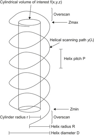 |
| Figure 41.1
Helical path of the X-ray source around the volume of interest.
|
41.2. Core Methods
Feldkamp
et al
.
[2]
proposed an efficient algorithm to perform filtered back projections for 3-D CT. Unfortunately, their algorithm was approximate and could introduce certain undesirable artifacts in the final reconstructed image. Katsevich
[4]
devised the first mathematically exact algorithm to reconstruct helical cone-beam CT images. The exactitude of the algorithm is before discretization. As for any mathematical algorithm, the computer precision will have an effect on the final result. A drawback of this algorithm is its computational complexity — when a volume of side
N
(i.e.,
N
×
N
×
N
volume) is reconstructed from
M
projections, its computational complexity will be of
O
(M
×
N
3
) order. This article addresses the computation time to reconstruct the images acquired by the cone-beam CT scanner by using start-of-the-art processing systems. We present parallelized and optimized implementations of the Katsevich algorithm on two popular platforms: generic IA-based multicore processors and the general-purpose graphics processing units (GPGPU) and then perform competitive analysis on their respective performance. The goal of this work is twofold. First, we will provide methodology, parallelization strategies, and coding optimization techniques to practitioners in the field of medical imaging. Second, we will shed new insight with regard to present performance glass jaws in the GPGPU hardware and provide recommendations to architects for improving future GPGPU designs.
41.3. Algorithms, Implementations, and Evaluations
In
[3]
, Fontaine and Lee provided details about the mathematical models of the Katsevich algorithm and demonstrated its basic implementation and parallelization, with several architectural optimizations at the algorithm level. We adopt similar parallelization strategy in this work.
Figure 41.2
depicts a high-level overview of the algorithm.
Briefly, image reconstruction is performed in three main steps, the differentiation, the filtering, and the back projection. The differentiation and the filtering steps prepare the acquired projections’ data to be back-projected onto the volume being reconstructed. X-ray beams that originate from the source, traverse the volume being imaged, and hit the detectors plane where their respective attenuations are measured. The acquired signal is known as projection data. The density of each element of the volume determines the attenuation factor, and therefore, the signal's value at a (u
,ω) location on the detector's plane. The reverse process, starting from the signal measured and determining the density of the medium traversed, is known as back projection.
Listing 41.1
shows a pseudo code of the steps taken from the acquired signal to the reconstructed volume. The differentiation step performs the multidimensional derivative along
u
,ω and the angle λ. When a flat detector screen is used, the X-rays that hit the screen's corners travel a longer distance than those that hit closer to the center. To account for this fact the differentiation step corrects the values by multiplying them by a weighting factor of
 . Filtering the projections after differentiation is acomplished in three steps: the forward mapping, the convolution with the kernel of the Hilbert transform, and the backward mapping. Any noncolinear three points in space uniquely define a plane. For a helical path defined by
 any three points located on it and separated by the same length (y
(λ),
y
(λ + ψ), and
y
(λ + 2ψ), where
any three points located on it and separated by the same length (y
(λ),
y
(λ + ψ), and
y
(λ + 2ψ), where
 ), will define a plane called a
κ
-plane. This plane intersects the detector's plane in a line known as Kappa line (κ
-line). There are
P
= 2
L
+ 1 discrete
κ
-lines defined by the angular increments
), will define a plane called a
κ
-plane. This plane intersects the detector's plane in a line known as Kappa line (κ
-line). There are
P
= 2
L
+ 1 discrete
κ
-lines defined by the angular increments
 where
l
∈ [−
L
,
L
] and
where
l
∈ [−
L
,
L
] and
 ;
R
and
r
are the radii of the helix and the volume of interest, respectively. Because the convolution needs to be performed along these lines, we need an operation that aligns the
κ
-lines onto horizontal rectilinear segments. This operation is known as the forward height re-binning.
Figure 41.3
shows these lines and the forward mapping. For a given projection, the forward mapping will be done according to the formula:
;
R
and
r
are the radii of the helix and the volume of interest, respectively. Because the convolution needs to be performed along these lines, we need an operation that aligns the
κ
-lines onto horizontal rectilinear segments. This operation is known as the forward height re-binning.
Figure 41.3
shows these lines and the forward mapping. For a given projection, the forward mapping will be done according to the formula:
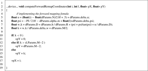
 where
u
is the coordinate along the horizontal axis on the detectors plane,
D
is the distance from the X-ray source to the detector's plane,
P
and
R
are the pitch of the helix and its radius, respectively, and ψ
l
is the angular discrete sampling as described earlier in this chapter.
where
u
is the coordinate along the horizontal axis on the detectors plane,
D
is the distance from the X-ray source to the detector's plane,
P
and
R
are the pitch of the helix and its radius, respectively, and ψ
l
is the angular discrete sampling as described earlier in this chapter.
(41.1)
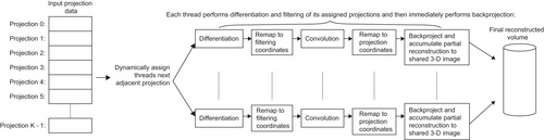 |
| Figure 41.2
Parallelization strategy for the cone-beam cover method.
|
After this remapping, the Hilbert transform is done on a row-by-row basis via a 1-D convolution with a special kernel
1
known as the Hilbert Transform Kernel. When all rows are convolved, the backward remapping step transforms the horizontal lines back to
κ
-lines. The backward mapping is done using a function
 , which is the inverse of ω(u
, ψ) defined by
Eq. 41.1
. At this stage, the projections are filtered and ready to be back-projected to construct the final volume. The second major step, and also the most time-consuming part of the entire computation, is the back projection. For any horizontal slice orthogonal to the z-axis of the volume under construction, there are a number of filtered back projections that will partially contribute to the final intensity value of each of the slice's voxels. We started by a single thread C implementation. After verifying its correctness we used its output as a reference against which we verified the results of the parallel implementations, on both a multicore CPU and the GPGPU. The filtering phase lends itself easily to parallelization.
, which is the inverse of ω(u
, ψ) defined by
Eq. 41.1
. At this stage, the projections are filtered and ready to be back-projected to construct the final volume. The second major step, and also the most time-consuming part of the entire computation, is the back projection. For any horizontal slice orthogonal to the z-axis of the volume under construction, there are a number of filtered back projections that will partially contribute to the final intensity value of each of the slice's voxels. We started by a single thread C implementation. After verifying its correctness we used its output as a reference against which we verified the results of the parallel implementations, on both a multicore CPU and the GPGPU. The filtering phase lends itself easily to parallelization.
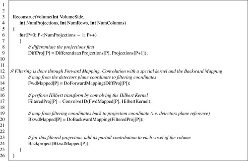 |
| Listing 41.1. |
| Pseudo code of the algorithm's implementation.
|
41.3.1. Projections’ Filtering
It may be helpful to consider a volume example so that we can refer to its dimension throughout the chapter. Let's consider reconstructing a volume of 512×512×512 voxels from 2560 projections, each of them 128 rows by 512 columns. In case of single-precision storage, the projection data size is 671,088,640 bytes large. The filtering operations cannot be done in place, and need temporary storage memory space. This shows the memory space requirements such applications put on the machine.
 |
| Figure 41.3
Kappa lines are mapped to parallel lines and back to Kappa lines.
|
Differentiation
When the GPGPU board has enough memory for all the projections and the temporary storage, we can process all the acquired data in a single kernel launch. Otherwise, we need to do it in a number of steps determined by the size of the data and the amount of available memory.
Listing 41.3
shows the excerpt of the differentiation kernel code. The dParams is a structure holding different needed parameters, and it is placed in the constant memory. We made this choice because all threads read the same parameters because they execute exactly the same code in a lockstep manner. The different parameters are computed on the host side from the information about the volume dimensions, and the projections it will be reconstructed from.
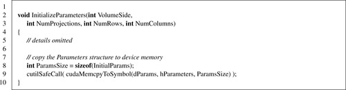
Listing 41.2
shows the code snippet that loads the initialized structure to the constant memory using
cudaMemcpyToSymbol
CUDA API. When certain information needs to be computed only once and can fit inside the constant memory, it may help performance to compute them a priori and store. The different threads reference a location rather than recomputing the value. This approach helps when the cost to compute the values in the saved table is higher than the cost to read it from the constant memory. For our example implementation, we saved trigonometric values for the projections’ angles in the constant memory. But when we applied the
––fast-math
flag to the compiler, the generated instruction for sin() and cos() were as fast as reading from the table.
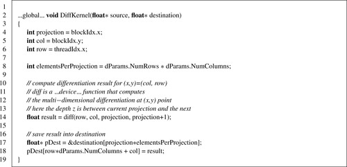 |
| Listing 41.3. |
| Differentiation kernel code.
|
The differentiation is done using the chain rule along the row, column, and neighboring projection, as
Figure 41.4
shows. This computation is implemented in the
diff
device function, which is called by the
DiffKernel
.
The limits of the maximum number of threads per block and the maximum extents on each dimension put restrictions on how to configure the computation grid on the GPGPU. For example, when differentiating 128×512 column projections, one cannot use
dim3 diffBlock(128, 512, 1)
because the maximum threads per block is 1024. Therefore, a valid kernel configuration needs to be something like
dim3 diffBlock(128, 1, 1); dim3 diffGrid(2560, 512).
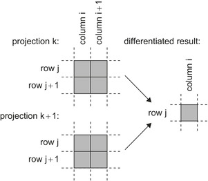 |
| Figure 41.4
Eight texels are required to compute the differential result.
|
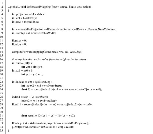
Forward Mapping
As mentioned earlier, we need to map the detectors that fall on the helical path into a horizontal line before we can apply the convolution with the Hilbert transform kernel. The forward-mapping tables can be computed a priori and stored, as done in the multicore CPU implementation. But for the GPGPU implementation, the constant memory is not large enough to hold the tables for a volume like 512
3
, and the global memory access is costly, so we adopted the approach of computing them on the fly as needed while performing the forward-mapping operation. The forward-mapping CUDA kernel is configured in a very similar way to the differentiation kernel, as can be seen from
Listings 41.4
and
41.5
.
computeForwardMappingCoordinates
implements the core of computing the forward mapping as described by the equation mentioned earlier and is listed in
Listing 41.6
.
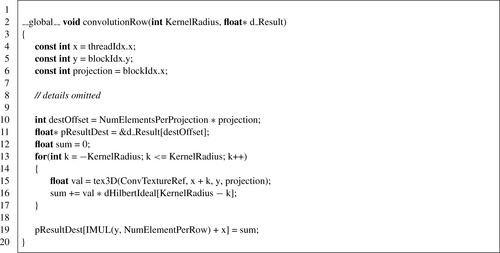
Convolution
After differentiation and forward-mapping operations, the projection is ready for the 1-D convolution for each of its rows. Each thread of a given block will compute the convolution result for a single pixel along a given row. The block will operate on each single row. Therefore, the kernel configuration will have a number of threads equal to the number of columns in each row. The configuration grid will be two-dimensional with the number of projections as the X dimension and the number of rows per projection as the Y dimension. Since the threads of a single block will operate on neighboring pixels, using textures to benefit from their caching support was an obvious choice. Therefore, the convolution step makes usage of a 3-D texture bound to the output memory of the forward-mapping operation as listed in
Listing 41.7
. The X and Y dimension matched the rows and columns of a projection, while the Z dimension matched the number of projections. It is worth noting that when the number of projections exceeds 2048, which is the limit on a 3-D texture, it is necessary to adopt a blocking approach and process the projections in subsets. A
cudaArray
was allocated and the results from the forward-mapping step copied to it. This device-to-device copying is necessary because of the use of
cudaArray
type. On the device side, the CUDA kernel that applies the convolution looks like
Listing 41.8
. Since the Hilbert transform kernel (dHilbertIdeal
in
Listing 41.8
) will be accessed by all threads, it was loaded into the constant memory to benefit from the fact that the threads of a warp accessing the same address will result in a single read. The read will be broadcast to all the thread members of the warp.
 |
| Listing 41.5. |
| Forward-mapping kernel launch configuration.
|
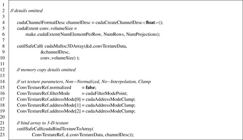 |
| Listing 41.7. |
| Binding a 3-D texture to convolution input memory.
|
Backward Mapping
The backward-mapping step brings the elements from the horizontal lines to the
κ
-lines. It is very similar in kernel launch configuration. The only difference is that it makes a call to the
computeBackwardRemapCoordinates
function instead of the forward-mapping one. This function
2
runs a loop to find the value of
 . After this step is completed, the projections can be sampled to add their respective contributions to each voxel of the volume under reconstruction.
41.3.2. Back Projection
To reconstruct the 512
3
volume mentioned earlier, in a single shot, we need to allocate enough memory to hold it, in addition to the memory required to hold the filtered projections. Therefore, we need:
 which is well above 1 GB of the device memory. This imposes the back projection to be performed in a blocked manner in the case of devices with less than 1.5 GB. The use of 3-D texture was motivated by the need to use the caching mechanism underlying the textures. The Katsevich algorithm uses sine and cosine trigonometric function to compute the sampling coordinates. These sampling coordinates are then used to read from the filtered projections. The use of trigonometric function in generating the memory access coordinates makes it very difficult, if not impossible, to come up with coalesced memory access pattern. When the size of the data working set can fit into the constant memory, it can help the performance to copy the data into the constant memory for reducing the cost of memory accesses. However, in this type of application, where a single projection in the example mentioned above is of size 256 kB, the use of constant memory is not possibile owing to the 64 kB size constraint. Therefore, we opted to use textures to take advantage of their underlying cache. But using textures comes with its constraints imposed by the GPGPU architecture and/or the CUDA API. For instance, in our implementation, the blocked approach we adopted was not because of the memory limitation, but owing to the fact that 3-D texture's coordinates cannot exceed 2048 in any given dimension. Because we use the Z-depth as the projection index, we had to constrain the number of projections loaded at once to be less than 2048. We reconstructed the volume in slices of a given thickness. When a slice between Z
1
and Z
2
coordinates is being reconstructed, not all projections are needed. In fact, only projections between a half-pitch under-scan below Z
1
and half-pitch over-scan above Z
2
are needed. For example, in the context of the 512
3
volume, a slice the thickness of 64 pixels requires 768 projections, not the whole 2560.
which is well above 1 GB of the device memory. This imposes the back projection to be performed in a blocked manner in the case of devices with less than 1.5 GB. The use of 3-D texture was motivated by the need to use the caching mechanism underlying the textures. The Katsevich algorithm uses sine and cosine trigonometric function to compute the sampling coordinates. These sampling coordinates are then used to read from the filtered projections. The use of trigonometric function in generating the memory access coordinates makes it very difficult, if not impossible, to come up with coalesced memory access pattern. When the size of the data working set can fit into the constant memory, it can help the performance to copy the data into the constant memory for reducing the cost of memory accesses. However, in this type of application, where a single projection in the example mentioned above is of size 256 kB, the use of constant memory is not possibile owing to the 64 kB size constraint. Therefore, we opted to use textures to take advantage of their underlying cache. But using textures comes with its constraints imposed by the GPGPU architecture and/or the CUDA API. For instance, in our implementation, the blocked approach we adopted was not because of the memory limitation, but owing to the fact that 3-D texture's coordinates cannot exceed 2048 in any given dimension. Because we use the Z-depth as the projection index, we had to constrain the number of projections loaded at once to be less than 2048. We reconstructed the volume in slices of a given thickness. When a slice between Z
1
and Z
2
coordinates is being reconstructed, not all projections are needed. In fact, only projections between a half-pitch under-scan below Z
1
and half-pitch over-scan above Z
2
are needed. For example, in the context of the 512
3
volume, a slice the thickness of 64 pixels requires 768 projections, not the whole 2560.
The parallelization of this step can be done in several different ways. First, we can set a block of threads to reconstruct a subvolume ([
x
0
x
1
], [
y
0
y
1
], [
z
0
z
1
]). The block of threads is set with dimensions (x
1
−
x
0
+ 1,
y
1
−
y
0
+ 1, 1), while the grid of blocks is set with (NumBlocksX
,
NumBlocksY
,1) for its dimensions, where
NumBlocksX
and
NumBlocksY
are the number of sub-blocks in the X and Y directions, respectively. Each thread in a given block will reconstruct the column [
z
0
z
1
] at location (x
,
y
) such that
x
0
≤
x
≤
x
1
and
y
0
≤
y
≤
y
1
. A second way of doing this is to have all the threads of the same block reconstruct the same column [
z
0
z
1
], and each block is set to build a given location (x
,
y
). The launch grid is configured as
dim3 BPGrid(volumeX, volumeY, 1)
, where
volumeX
and
volumeY
are the volume dimensions in the X and Y directions, respectively. The latter method rendered better performance than the former. This is due mainly to the fact that the coordinates (x
,
y
) affect the values of the sampling coordinates, while the
z
level does not. When the threads of a given block are constructing the column [
z
0
z
1
], they sample a given projection at the same (u
,
w
) position. This benefits from the spatial locality offered by the cache underlying the textures. This method reconstructed the volume in one-third of the time taken by the former one. To summarize, each thread of a block (x
,
y
) reconstructs the voxel at level
z
by looping through all the necessary projections. A third way of reconstructing a slice of the volume is to parallelize the computation along the projections, in other words, to make each thread compute the partial contributions of a subset of the projections. This approach requires reduction to generate the final density value of a given voxel. Besides the location (x
,
y
), the other factor that affects sampling coordinates values is the angle at which the projection was taken. Because these threads handle different projections, they use different sampling coordinates and, hence, they cannot take advantage of memory locality. These are part of the reason why this third approach runs slower than the second. The other factor is the fact that the needed reduction step to generate voxel densities is to be done in the shared memory; hence, the number of threads per block is limited by the size of the shared memory and the number of elements per column being reconstructed. Another reason that the second approach performed better than the other two is the complete elimination of the need for global synchronization. This absence of interdependence between the threads allows them to make forward progress as fast as the GPU clock permits. For GPU applications, any algorithm's implementation that needs to take care of memory coherency will suffer significantly because the memory accesses will become a serialization point in the computation flow. Eliminating, or at least reducing, the need for global synchronization is a key optimization for GPGPU applications.
Listing 41.9
shows the second method described earlier. Each thread loops through all projections and reconstructs a single voxel of the volume; therefore, we avoided the coherency issue that arises from the cooperative construction of a voxel by multiple threads.
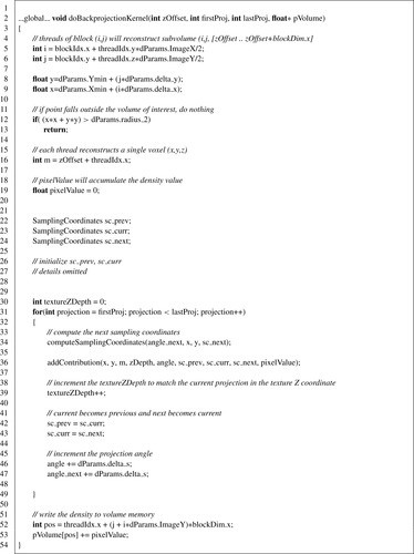
The function
addContribution
3
samples the 3-D texture and returns the contribution from a particular filtered projection to the current (x
,
y
,
z
) voxel. We organized the 3-D texture by making each filtered projection a slice in it. When the GPGPU device's global memory can hold all the projections for the volume being reconstructed, we load all of them. If not, we load just a number of them per kernel launch, and we perform a number of launches to complete the back projection. Even when there is enough memory to hold all the filtered data, we could not do it because the CUDA implementation does not allow more than 2048 per dimension. It would be helpful to have a flexible texture extension setup. For example, to have a 2048×2048×2048 3-D texture or a 512×512×8192. The texture-sampling facility offers two types of
cudaTextureFilterMode
,
cudaFilterModePoint
and
cudaFilterModeLinear
. When the linear interpolation mode is set, the type of interpolation is determined by the dimensionality of the texture. CUDA provides a template to declare texture reference objects of different dimensions. The statement
texture < float, 2, cudaReadModeElementType > texRef2D
, for example, declares a 2-D texture reference object using floats as the underlying type. The statment
texRef.filterMode = cudaFilterModeLinear;
is used when the programmer wants to use hardware interpolation. The type of linear interpolation, that is, 1-D, 2-D, or 3-D interpolation, is inferred from the texture type, which is defined by the dimension parameter passed to the texture template. It is very common to use 3-D textures for the sole purpose of stacking a number of 2-D textures. In this case the programmer may still want to use hardware linear interpolation in the 2-D sense even if the texture object is declared of type 3-D, because the intent of using 3-D texture is just to stack many 2-D textures, not to use it for 3-D sampling. But setting the filter mode to linear will cause the hardware interpolator to use eight elements, four elements from each of two neighboring 2-D textures. It would be a good addition to CUDA to let the programmer specify the dimensionality of interpolation when 2-D or 3-D texture references are used. A call like
texRef3D.filterMode = cudaFilterModeLinear2D
, where the texture reference is declared as
texture<float, 3, cudaReadModeElementType> texRef3D;
would mean that 2-D linear interpolation is wanted on the X-Y plane only. The hardware interpolator would pick the nearest 2-D texture to the given Z level and sample it using the 2-D linear interpolation.
The statment
float sample = tex3D(texRef3D, u, v, w);
should return the 2-D linearly interpolated value of the four neighbors of position (u, v) on the 2-D projection corresponding to the Z level closest to w.
41.4. Final Evaluation and Validation of Results, Total Benefits, and Limitations
Different GPGPU devices were used to test our implementation, including a Tesla C870 containing 16 streaming multiprocessors (SMs) with eight cores on each that amounts to a total of 128 cores, a Tesla C1060 containing 30 SMs with eight cores on each, and the new Fermi-based GTX 480 with 480 cores distributed between 60 SMs. We performed comparison among the implementations of the same algorithm. In this case, the cone-beam cover method was implemented on the multicore CPU using OpenMP and Intel Compiler and Intel's IPP library. The multicore CPU speedup numbers are for the cone-beam cover method between a single thread and eight-thread parallel version. The performance of the eight-thread multicore version was measured on a dual-socket quad-core Clovertown processor running at 2.33 GHz.
Table 41.1
summaries our performance measurement for the CPU implementation and the best of the breed GPGPU implementation running on GTX 480.
The results collected from the GTX 480 with comparison to the basic single-core and the multicore CPU implementations are presented for different cubic volumes in the same table. In ideal conditions (i.e., assuming a perfect memory subsystem), the multithreaded version should manifest the same speedup no matter what the volume size is. For the cases running on the multicore CPU, the cache hierarchy plays a critical role in the whole performance; therefore, the program suffers a certain penalty when large data is handled to reconstruct the image. Because the cache capacity misses are responsible for the penalty, having many threads available to perform computation alleviates the penalty by partially hiding it through parallelism. Hence, a part of the speedup from the multithreaded CPU code is due to the number of threads running in parallel; the other part of the speedup is due to partially hiding the cache misses penalty. For this reason, the 8T CPU code shows a superlinear speedup with reference to the single-thread version. In the cases of GPGPU, the existence of level of parallelism and a high enough ratio of computation-to-memory access can hide the memory access penalty. Because our implementation on the GPGPU is completely parallelized, the reconstruction time looks more interesting when large volumes are used. Nonetheless, it is noticeable that the speedup trend did not continue when we reconstruct the largest volume in our experiment: 1024
3
. Reconstructing such large volume incurs many more round-trips between the host and the device than for smaller volumes. Copying memory by small chunks carries some penalty compared with moving all the data at once. In addition, making many trips between the host and the device requires synchronization using the
cudaThreadSynchronize
API. As an example the reconstruction of 1024
3
costs 160 seconds just for copying memory between the host and device.
To see how the performance of GPGPU implementation scales with the number of cores, we collected the results from several GPGPUs with a different number of cores. The Tesla C870 has 128 cores, the Tesla C1060 has 240 cores, and the GTX 480 has 480 cores. To show only the effect of the number of cores per device over the speedup, the same memory loads are used on all devices. For example, when we reconstruct a 1024
3
volume, memory is a decisive parameter on speedup; for this reason, even when it is possible to load larger datasets at once onto the Tesla C1060 that has a larger global memory size of 4 GB, we restricted the partial datasets to be of the same size as on the Tesla C870 and the GTX 480, both of which have only 1.5 GB of global memory.
Table 41.2
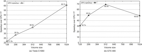
shows how the same application code performs on GPGPU devices with a different number of cores and shows their corresponding scaling trend. The speedups as a function of the volume are reported in
Figures 41.5(a)
and
41.5(b)
for the Tesla C1060 and the GTX 480, respectively.
 |
| Figure 41.5
GPGPU speedup trend.
|
When we are reconstructing large volumes, a good amount of time is spent in transferring data because it is done in partial amounts that can fit in the GPU device memory. For example, the 1024
3
volume reconstruction consumes 152 seconds in data transfer and extra round-trips between the host and the device.
Unlike the case of the Tesla C1060 with 4GB memory (Figure 41.5(a)
), the speedup chart of the GTX 480 (Figure 41.5(b)
) did not continue the trend at the 1024
3
volume. This is mainly due to the multiple round-trips penalty of 152 seconds. If we consider reconstruction time only, the speedup would be a little more than 60 times.
41.4.1. A Note on Energy Consumption
The multithreaded multicore CPU version was run on a dual-socket Clovertown processor at 2.33 GHz (each processor has a total power consumption of 80 watts as stated on Intel's Web site). The best performance on the GPGPU was given by the GTX-480 board, which has a total power consumption of 250 watts. The Tesla C870 has a total power consumption of 170 watts, while the Tesla C1060 board is rated at 187.8 watts. The maximum power dissipations for the different GPUs are collected from their respective brochures provided by NVIDIA. We used the maximum power dissipation as a ballpark estimate for the energy consumed. These numbers are by no means definitive, nor are they measured experimentally. They are simply a rough guess of the energy consumption neighborhood. There is an implicit assumption that the CPU or GPU will dissipate the peak power value while performing the computation.
Table 41.3
shows how many joules it took to reconstruct each volume for the eight-threads CPU version and for the GPGPU version. Even though the power consumption of the GPGPU is much higher than that of the CPU multicore system, the energy dissipated to accomplish the same job, nonetheless, is much smaller on the GPGPU. This is not surprising because the SM design of a GPGPU is much more computationally efficient. On average, we observed energy savings from 9.5% to 70.3% depending on the size of volume being reconstructed and the GPU device used. The GTX-480 shows the highest energy savings except for the 1024
3
volume where C1060 GPU was better. This is because the GTX-480 board used in the experiments has only 1.5GB of memory, and more seconds were paid for the extra transfers. The energy cost benefits of using GPUs for applications that can be implemented in a heavily parallel ways are quite evident. This also justifies the current industry trend of integrating more diversified accelerators on chip to improve the overall energy efficiency of computation.
41.5. Related Work
Owens
et al
.
[7]
surveyed and categorized the development of general-purpose computation on graphics processors and demonstrated the potential of their enormous computation capability. Regarding the CT image reconstruction work, Noo
et al
.
[6]
discussed the Katsevich algorithm for both the curved and flat panel detectors and presented an implementation strategy for these two types of CT scanners. Deng
et al
.
[1]
describe a parallel implementation scheme of the reconstruction algorithm on a 32-node cluster of 64-bit AMD Opteron processors. Fontaine and Lee
[3]
studied the parallelization of the Katsevich CT image reconstruction method using Intel multicore processors. Their OpenMP implementation was used in this chapter for comparison against the CUDA results on three different GPGPUs. Lee
et al
.
[5]
present a comparative study of applications on GPU and multicore CPU platforms. Results from a set of throughput computing kernels are presented to show how the performance of an Intel Core i7-960 processor compares with that of an NVIDIA GTX280. The optimizations on each platform are also discussed. Recently, more works have been done by using GPGPU to improve the performance of medical imaging reconstruction. For example, Stone
et al
.
[9]
presented the use of GPGPUs in the acceleration of image reconstruction from the magnetic resonance imaging (MRI) machines. Sharp
et al
.
[8]
studied the acceleration of the cone-beam CT image reconstruction method using the Brooks programming environment on an NVIDIA 8800 GPU, but adopted the older, nonexact FDK algorithm in their study. Xu
et al
.
[10]
studied the feasibility of real-time 3-D reconstruction of CT images using commodity graphics hardware. A parallel implementation of the Katsevich algorithm on GPU is presented in
[11]
. Yan
et al
. developed a minimal overscan formula and explained an implementation using both CPU and GPU. Their application performed the projection's filtering on the CPU and the back projection on the GPU graphics pipeline. Zhou and Pan
[12]
proposed an algorithm based on the filtered back-projection approach that requires less data than the quasi-exact and exact algorithms.
41.6. Future Directions
The presented work shows how a fully parallel implementation of a given algorithm takes full advantage of the GPGPU architectures and how it scales with no need to change the code. A similar experiment can be done for the symmetry method proposed in
[3]
. This method requires rearrangement of the projections after filtering to make the ones that are separated by an angle of
 column interleaved. After this shuffling, the sampling can be done in 128-bit wide elements (i.e.,
float4
), and four voxels will be reconstructed at once. Fontaine and Lee's paper provides detailed explanations with respect to how it was done with their algorithmic level optimization (inherent symmetry), as well as the application of SIMD ISA provided by the IA-based processors. It is expected that this algorithm will show similar speedups.
column interleaved. After this shuffling, the sampling can be done in 128-bit wide elements (i.e.,
float4
), and four voxels will be reconstructed at once. Fontaine and Lee's paper provides detailed explanations with respect to how it was done with their algorithmic level optimization (inherent symmetry), as well as the application of SIMD ISA provided by the IA-based processors. It is expected that this algorithm will show similar speedups.
41.7. Summary
Medical image processing applications are not just computation intensive; they also require a large amount of memory for both original data storage and temporary data processing. When the implementation of a given algorithm can completely be parallelized, it will likely benefit from the availability of more processing cores to scale performance given the memory overheads are negligible. It may even be beneficial to sacrifice certain optimization opportunities to allow full parallel implementation of the algorithm. In this article, we used the Katsevich CT image reconstruction algorithm as an application to demonstrate how modern multicore and GPGPU processors can substantially improve the performance of medical image processing. We also identified the limited size of device memory to be a performance glass jaw that prevents the scalability of speedup as the input data set becomes larger. Not having enough memory to hold all the volumes being reconstructed and their intermediate results requires high bandwidth between the host and the GPGPU, leading to substantial performance degradation.
[1]
J. Deng, H. Yu, J. Ni, T. He, S. Zhao, L. Wang,
et al.
,
A parallel implementation of the Katsevich algorithm for 3-D CT image reconstruction
,
J. Supercomput.
38
(1
) (2006
)
35
–
47
.
[2]
L. Feldkamp, L. Davis, J. Kress,
Practical cone-beam algorithm
,
J. Opt. Soc. Am. A
1
(6
) (1984
)
612
–
619
.
[3]
E. Fontaine, H.-H.S. Lee,
Optimizing Katsevich image reconstruction algorithm on multicore processors
,
In:
Proceedings of 2007 International Conference on Parallel and Distributed Systems
,
vol. 2
(2007
)
Kaohsiung
,
Taiwan
, pp.
1
–
8
.
[4]
A. Katsevich,
Theoretically exact filtered backprojection-type inversion algorithm for Spiral CT
,
SIAM J. Appl. Math.
62
(2002
)
2012
–
2026
.
[5]
V.W. Lee, C. Kim, J. Chhugani, M. Deisher, D. Kim, A.-D. Nguyen,
et al.
,
Debunking the 100X GPU vs. CPU myth: an evaluation of throughput computing on CPU and GPU
,
In:
ISCA '10: Proceedings of the 37th Annual International Symposium on Computer Architecture
ACM, New York
. (2010
), pp.
451
–
460
.
[6]
F. Noo, J. Pack, D. Heuscher,
Exact helical reconstruction using native cone-beam geometries
,
Phys. Med. Biol.
48
(23
) (2003
)
3787
–
3818
.
[7]
J.D. Owens, D. Luebke, N. Govindaraju, M. Harris, J. Kruger, A. Lefohn,
et al.
,
A survey of general-purpose computation on graphics hardware
,
Comput. Graph. Forum
26
(1
) (2007
)
80
–
113
.
[8]
G. Sharp, N. Kandasamy, H. Singh, M. Folkert,
GPU-based streaming architectures for fast cone-beam CT image reconstruction and demons deformable registration
,
Phys. Med. Biol.
52
(2007
)
5771
.
[9]
S. Stone, J. Haldar, S. Tsao, W. Hwu, B. Sutton, Z. Liang,
Accelerating advanced MRI reconstructions on GPUs
,
J. Parallel Distrib. Comput.
68
(10
) (2008
)
1307
–
1318
.
[10]
F. Xu, K. Mueller,
Real-time 3D computed tomographic reconstruction using commodity graphics hardware
,
Phys. Med. Biol.
52
(12
) (2007
)
3405
.
[11]
G. Yan, J. Yian, S. Zhu, C. Qin, Y. Dai, F. Yang,
et al.
,
Fast Katsevich algorithm based on GPU for helical cone-beam computed tomography
,
IEEE Trans. Inf. Technol. Biomed.
14
(4
) (2010
)
1053
–
1061
.
[12]
Y. Zhou, X. Pan,
Exact image reconstruction on PI-lines from minimum data in helical cone-beam CT
,
Phys. Med. Biol.
49
(2004
)
941
–
959
.
..................Content has been hidden....................
You can't read the all page of ebook, please click here login for view all page.