Data Warehousing Revisited
The information links are like nerves that pervade and help to animate the human organism. The sensors and monitors are analogous to the human senses that put us in touch with the world. Databases correspond to memory; the information processors perform the function of human reasoning and comprehension. Once the postmodern infrastructure is reasonably integrated, it will greatly exceed human intelligence in reach, acuity, capacity, and precision.
—Albert Borgman, Crossing the Postmodern Divide. Chicago: University of Chicago Press, 1992.
Introduction
The first part of this book introduced the world of Big Data; its complexities, processing techniques, and technologies; and case studies on Big Data. This chapter reintroduces you to the world of data warehousing. We look at the concept and evolution of the data warehouse over the last three decades. Since the days of punch cards to the writing of this book, there has been one fundamental struggle: managing data and deriving timely value. The last three decades have created many tipping points in technology that have evolved the growth of data management including data warehousing. Companies have invested millions of dollars into creating data warehouses and these investments need to be leveraged for solving the right problems.
Prior to the advent of electronic data processing, companies used to manage their customers more by customer loyalty of making purchases at the same store for products, and used to track inventory using traditional bookkeeping methods. At that time, population demographics were small and buying trends for products and services were limited. When the early days of electronic data processing came about in the early 1950s, initial systems were based on punch cards. The benefit of the systems was their ability to start managing pockets of businesses in electronic formats. The downside was the proliferation of multiple stores of data on punch cards that reflected different values, and damage to the paper would mean loss of data. We quickly evolved from the punch cards to magnetic tapes that gave better data storage techniques, yet were not able to control the proliferation of different formats of data. From magnetic tapes we evolved to disks where we could store data. Along the way the applications that generated and controlled data production from the front-end perspective moved quickly from simple niche languages to declarative programming languages.
Tracking along the progress of the storage and programming languages, the applications to manage customers, employees, inventory, suppliers, finances, and sales evolved. The only issue with the data was it could not be analyzed for historical trends, as the data was updated in multiple cycles. Thus evolved the first generation of OLTP applications. Around the same time in the 1970s, Edgar. F. Codd published his paper on the relational model of systems for managing data.1 The paper was pivotal in several ways:
• It introduced for the first time a relationship-based approach to understanding data.
• It introduced the first approach to modeling data.
• It introduced the idea of abstracting the management and storage of data from the user.
• It discussed the idea of isolating applications and data.
• It discussed the idea of removing duplicates and reducing redundancy.
Codd’s paper and the release of System R, the first experimental relational database, provided the first glimpse of moving to a relational model of database systems. The subsequent emergence of multiple relational databases, such as Oracle RDB, Sybase, and SQL/DS, within a few years of the 1980s were coupled with the first editions of SQL language. OLTP systems started emerging stronger on the relational model; for the first time companies were presented with two-tier applications where the graphical user interface (GUI) was powerful enough to model front-end needs and the underlying data was completely encapsulated from the end user.
In the late 1970s and early 1980s, the first concepts of data warehousing emerged with the need to store and analyze the data from the OLTP. The ability to gather transactions, products, services, and locations over a period of time started providing interesting capabilities to companies that were never there in the OLTP world, partially due to the design of the OLTP and due to the limitations with the scalability of the infrastructure.
Traditional data warehousing, or data warehousing 1.0
In the early days of OLTP systems, there were multiple applications that were developed by companies to solve different data needs. This was good from the company’s perspective because systems processed data quickly and returned results, but the downside was the results from two systems did not match. For example, one system would report sales to be $5,000 for the day and another would report $35,000 for the day, for the same data. Reconciliation of data across the systems proved to be a nightmare.
The definition of a data warehouse by Bill Inmon that is accepted as the standard by the industry states that the data warehouse is a subject-oriented, nonvolatile, integrated, time-variant collection of data in support of management’s decision.2
The first generation of data warehouses that we have built and continue to build are tightly tied to the relational model and follow the principles of Codd’s data rules. There are two parts to the data warehouse in the design and architecture. The first part deals with the data architecture and processing; per Codd’s paper, it answers the data encapsulation from the user. The second part deals with the database architecture, infrastructure, and system architecture. Let us take a quick overview of the data architecture and the infrastructure of the data warehouse before we discuss the challenges and pitfalls of traditional data warehousing.
Data architecture
From the perspective of the data warehouse, the data architecture includes the key steps of acquiring, modeling, cleansing, preprocessing, processing, and integrating data from the source to the EDW outlined here:
1. Business requirements analysis:
• In this step the key business requirements are gathered from business users and sponsors.
• The requirements will outline the needs for data from an analysis perspective.
• The requirements will outline the needs for data availability, accessibility, and security.
• In this step the data from the OLTP is analyzed for data types, business rules, quality, and granularity.
• Any special requirements for data are discovered and documented in this step.
• In this step the data from the OLTP models are converted to a relational model. The modeling approach can be 3NF, star schema, or snowflake.
• The key subject areas and their relationships are designed.
• The hierarchies are defined.
• The physical database design is foundationally done in this step.
• The staging schema is created.
• If an ODS is defined and modeled, the ODS data model is defined and created.
• In this step the process of extracting, loading, and transformation of data is designed, developed, and implemented.
• There are three distinct processes developed typically; some designs may do less and others will do more, but the fundamental steps are:
– Staging extract and EDW loading
• Data transformations are applied in this phase to transform from the OLTP to the EDW model of data.
• Any errors occurring in this stage of processing are captured and processed later.
• Data movement and processing will need to be audited for accuracy and a count of data along each step of the process. This is typically accomplished by implementing an audit, balance, and control process to trace data from the point of arrival into the data warehouse to its final delivery to datamarts and analytical data stores.
• In this step, typically done both in the ETL steps and in the staging database, the data from the source databases is scrubbed to remove any data-quality issues that will eventually lead to data corruption or referential integrity issues.
• To enable data quality, there are special third-party tools that can be deployed.
• Errors in this step are critical to be discovered and marked for reprocessing.
• In this step all the key staging to EDW data transformation rules are processed.
• Data aggregations and summarizations are applied.
• Data encryption rules are applied.
• In this step the data presentation layers including views and other semantic layers are readied for user access.
Infrastructure
The data architecture of a data warehouse is the key to the castle of knowledge that lies within, but the infrastructure of a data warehouse is the castle. The data warehouse architecture from an infrastructure perspective consists of the following as shown in Figure 6.1:
• Source systems—these represent the various source feeds for the data warehouse.
• Data movement (ETL/CDC) —this represents the primary programming techniques of moving data within the ecosystem.
• Databases—there are several databases created and deployed within the data warehouse:
• Staging areas—these databases (in some instances, there is more than one staging database to accommodate data from different sources) are the primary landing and preprocessing zone for all the data that needs to be moved into the data warehouse.
• Operational data store—this database represents the database structure extremely close to the source systems and is used as an integration point for daily data processing. Not all data warehouses have an ODS.
• (Enterprise) data warehouse—the data warehouse is arguably one of the largest databases in the enterprise. It holds many years of data from multiple sources combined into one giant structure.
• Datamarts—these are specialty databases that are designed and developed for use by specific business units and line of business in the enterprise. In a bottom-up approach to data warehousing, enterprises build multiple datamarts and integrate them.
• Analytical database—these are databases that extract or copy data from the data warehouse and support analytical platforms for data mining and exploration activities.

The analytical databases are deployed on a combination of infrastructure technologies including:
• Traditional data warehouses are developed on RDBMS technologies like Oracle, SQL Server, DB2, and Teradata.
• There are niche solutions built on DBMS technologies like Ingres, PostGres, and Sybase.
• Enterprise network connections based on 10 MB/100 MB pipes.
• SAN (storage area network) is the most common storage platform.
• All the data across the enterprise typically shares the SAN in a partitioned allocation.
• Smaller data warehouses can be stored on NAS (network-attached storage).
• Data warehouse, datamart, and analytical database server infrastructure can be deployed on
– Unix operating systems: 32-/64-bit with 4, 8, or 16 dual-core CPUs, some use quad-core processors, 8, 16, 64, or 128 GB of DDR3 RAM.
– Linux operating systems: 32-/64-bit with 4, 8, or 16 dual-core CPUs, some use quad-core processors, 8, 16, 64, or 128 GB of DDR3 RAM.
– Windows operating systems: 32-/64-bit with 4, 8, 16 dual-core CPUs, some use quad-core processors, 8, 16, 64, or 128 GB of DDR3 RAM.
• There are instances where a large server is partitioned into multiple virtual servers and shared between the different components.
These are all the different moving parts within any data warehouse, and upkeep of performance of these components is a major deterrent for enterprises today.
Pitfalls of data warehousing
Is your data warehouse implementation and adoption a success? When asked this question, a large number of data warehouse implementations often cite failure with the implementation because performance becomes a real challenge over a period of time, depending on the size and complexity of transformations within the processing layers in the data warehouse. The underlying reason for performance and scalability issues is the sharing of resources in the infrastructure layer and the database layers. In Figure 6.1, you can see the following layers of shared infrastructure:
• The source database is isolated in its own storage, though it is a partition of a larger storage cluster.
• The ODS (if deployed), staging, and EDW databases are all normally connected to one storage architecture.
• The physical servers for the staging and EDW are the same system and database servers.
• This shared infrastructure creates scalability and performance issues:
– The I/O is constrained in the same enterprise network pipe.
– The I/O between the source, staging, and EDW databases needs to travel from source, to staging, to ETL, to storage, to ETL, to EDW. A lot of system resources and the network are dedicated to managing this dataflow and it introduces natural time latencies.
– Timeouts on connections, slow-moving transactions, and outages on disk architecture are other common side effects that occur in this environment.
• The server hardware can be a set of virtual partitions on a large physical server.
• The staging and EDW databases are normally in one server.
• Analytical databases are normally installed in their own server environment.
Performance
What is the limitation of sharing-everything architecture? The answer to this lies in understanding the shared-everything architecture as shown in Figure 6.2. In this architecture:
• Memory, CPU, and system bus are shared by all programs running on the systems.
• Storage is shared across the programs.
• The network is a common enterprise network and not a direct tethered connection in most cases.
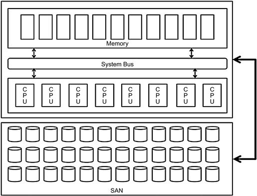
The architecture approach described in Figure 6.2 is not the optimal architecture to handle the large volume of data, the processing complexities, and users defined for the data warehouse. This architecture will scale well and perform with consistency on an OLTP or transaction processing platform, since the transactions are discrete in size and occur in small bursts. The system can be tuned and maintained for optimal performance and managed to accommodate the growth needs of a transactional environment.
The data warehouse is a collection of transactional data over a period of time and by definition is a larger data set, which will be used for a variety of query and analysis purposes by multiple users in an enterprise.
In a shared-services environment, there are several issues that limit the performance and scalability of the data warehouse. Let us examine the performance aspect of the data warehouse versus the OLTP platforms in the shared environment.
In an OLTP query execution, classic transactional queries are discrete like:
• Insert into Sales(date, gross_sales_amt, location_id, product_code, tax_amt)
If you observe the query pattern, you can discern that for each of these query actions a particular record in a table will be affected. This activity typically generates a roundtrip across the different infrastructure layers and does not timeout or abruptly quit processing, since the data activity is record by record and each activity is maintained in a buffer until the transaction commit is accomplished. There can be many such small queries that can be processed on the OLTP system, since the workload performed in this environment is small and discrete.
The amount of CPU cycles, memory consumed, and data volume transported between the server and storage can be collectively expressed as a unit of “workload” (remember this definition, as we will discuss it over the next few chapters in greater depth).
Now let us look at the execution of a query on the data warehouse data set. Typically, the query will take a longer processing cycle and consume more resources to complete the operation. This can be attributed to the size of the data set and the amount of cycles of transportation of data across the different layers for processing, compiling, and processing the final result set, and presentation of the same to the process or user requesting the query. The data warehouse can handle many such queries and process them, but it needs a more robust workload management design, as the resources to process the data of this size and scale will differ from the OLTP environment. There is a different class of workload that will be generated when you process data from web applications within the data warehouse environment and another class of workload for analytical query processing.
Continuing on understanding how workloads can impact the performance, for a transactional query the workload is streamlined and can be compared to automobiles on expressways. There is a smooth flow of traffic and all drivers follow lane management principles. The flow is interrupted when a breakdown, accident, or large volume of big rigs merge in the traffic. On a similar note, you will see a slowdown or failure of query processing if there is an infrastructure breakdown or a large and complex query that might have been generated by an ad-hoc user, which will resemble traffic jams on any large-city expressway when an accident occurs.
The hidden complexities of data warehouse queries are not discernable by visual inspection. The reason for this is the design and architecture of the semantic layers built on top of the data warehouse, which allows the user to navigate the relationships in the underlying data and ask questions that can drive workload and optimization demands in multiple layers, and sometimes creates conflicts between the optimization and its workload model in the database.
For example, to determine the sales dollars per month and year for each customer in a household, the query on a data warehouse will look as follows:
Select cust.customer_name, cust.cust_id, household.household_id, household.state, sum(sales.net_sales_amt) net_sales, sales.month_num, sales.year_num from cust,household,sales where cust.household_id = household.household_id and cust.cust_id = sales.cust_id group by cust.customer_name, cust.cust_id, household.household_id, sales.month_num, sales.year_num
Let us assume the tables sizes are:
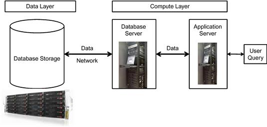
To execute this query, the data warehouse will perform several cycles of computational processing across layers of infrastructure, as shown in Figure 6.3:
• There are large data sets that will be read from the disk and moved to the memory and back to the disk. This will lead to excessive data swapping between different layers on a continued basis.
• Additionally, the same data may be needed multiple times and depending on how stale or fresh the data is, the query might have to repeat the processing steps since there is not enough space to persist the result sets.
• Depending on the configuration setting of the database and the server, the memory and CPU are divided between the multiple threads that are generated by the query for processing. For example, a dual-core CPU can execute four threads—two per CPU. In the case of an average server the CPU can execute 32 threads for eight CPUs. If there are 32 threads and eight users running, the CPU cycles will be divided for the eight users.
• If there are multiple queries executing operations in parallel, there will be contention for resources, as everybody will be on the same shared-everything architecture. Multiple threads of execution can decrease throughput and increase swapping of data and slowdown of execution.
• If the data warehouse load operations execute in parallel with the query processing, they can evolve into sync issues especially in circular references.
• A mix of query and load operations can cause the database to underperform in the shared architecture as it creates a mixed workload.
• Adding ad-hoc users and data mining type of operations can cause further underperformance.
The challenge of the shared-everything architecture limits the usability of the data warehouse. The data warehouse can underperform due to growth of data, users, queries, load cycles, new applications like data mining, and online analytical processing (OLAP). The problem manifests after three to six months in a high-volume database, and in a year in a lower-volume database. How do organizations address this situation? In addition to the performance issues, the scalability challenge is another area that is a constant threat.
Typically, the next step a database administrator and system administrator take is performance tuning the data warehouse. Adding indexes, storage, and server capacities are the most common techniques. With all this performance tuning, there are still challenges that limit the adoption of the data warehouse. The reason for this situation is that all these actions are being done in the same shared-everything infrastructure. The end result is momentary relief and not radical sustained performance. These issues remain whether you build the data warehouse using top-down or bottom-up approaches.
While performance is one major area that continues to challenge the data warehouse, scalability is another area that has been a significant challenge to the success of data warehouses. In the next section we will discuss the scalability issues and how they have been addressed.
Scalability
Database scalability is commonly used to define improvements in the infrastructure and data structure areas of the data warehouse to accommodate growth. Growth in the data warehouse happens in two areas: the volume of data and new data, and the growth of users across different user hierarchies. Both of these situations affect the performance and the scalability of the database. Common techniques to scale up performance in a shared-everything architecture include:
• Adding more server hardware. You need to scale up both the CPU and memory for achieving some benefit; scaling one component does not provide huge benefits.
• Adding more storage does not help if you cannot separate the data structures discreetly into their own specific substorage areas.
• Implementing a robust data management technique, by reducing the amount of data in the tables by archiving history, can help only if volumes are extremely high.
• Creating additional indexing strategies normally creates more overhead than help.
• Compressing data on storage with the available compression algorithms.
• Create aggregate tables or materialized views.
• Archiving data based on usage and access. This differs from the traditional archiving techniques where data is archived based on a calendar.
The performance of a database can be definitely improved by a combination of effective data management strategies, coupled with a boost in additional hardware and storage. By this technique you can achieve efficiencies of processing and execution of tasks.
In a shared-everything architecture, as you improve the efficiencies of processing on the server hardware, the storage layer also needs to be parallelized. Techniques for managing and improvising storage architecture include:
• Another implementation of multinode concept.
• All writes are written to the master.
• All reads are performed against the replicated slave databases.
• Is a limited success, as large data sets slow down the query performance as the master needs to duplicate data to the slaves.
• Master and slave databases are synced on a continuous basis, causing query performance and result set consistency issues.
• Create many nodes or clones.
• Each node is a master and connects to peers.
• Any node can service a client request.
• Did not emerge as a big success for RDBMS:
– Consistency was loosely coupled.
– ACID principles violated data integrity.
• Partitioning of data has been a very popular option supported by the database vendors, even though the scalability achieved is limited due to inherent design limitations. With partitioning:
• Data can be partitioned across multiple disks for parallel I/O.
• Individual relational operations (e.g., sort, join, aggregation) can be executed in parallel in a partitioned environment, as resources can be bequeathed to the operation.
• Commonly used partitioning techniques are:
– Based on a list of values that are randomly applied.
– Applied when a single table cannot sit on a server.
– Split table onto multiple servers based on ranges of values; commonly used ranges are dates.
• Key or hash-based partitioning:
– In this technique, a key-value pair is used in the hash partitioning and the result set is used in the other servers.
a. First partition of the table by hash keys.
b. Subpartition by range of values.
The partitioning techniques introduce a different problem in the storage architecture, the skewing of the database. Certain partitions may be very large and others small, and this will generate suboptimal execution plans.
The following are partitioning methods that are used for large tables:
• Partition large tables by columns across the database, normally in the same database.
• The biggest issue with this technique is that we have to balance the partition when the tables grow in columns.
• Queries needing large columns will fail to perform.
• The technique will not scale for data warehousing, but lends well for OLTP.
• Tables are partitioned by rows and distributed across servers or nodes in a database.
• Queries looking for more than one group of rows will have to read multiple nodes or servers.
• Extremely large tables will be heavily skewed in this distribution.
Partitioning, adding infrastructure, and optimizing queries do not enable unlimited scalability in the data warehouse for extremely large data. The workarounds used to enhance scalability and performance include:
• Designing and deploying multiple data warehouses for different business units or line of business (defeats the purpose of an integrated data warehouse).
• Deploy multiple datamarts (increases architecture complexity).
• Deploy different types of databases to solve different performance needs (very maintenance-prone).
The evolution of the data warehouse appliance and cloud and data virtualization has created a new set of platforms and deployment options, which can be leveraged to reengineer or extend the data warehouse for sustained performance and scalability. We will be looking at these technologies and the reengineering techniques in the next few chapters.
Architecture approaches to building a data warehouse
The last area of overview in this chapter is the data warehouse building approaches with different architecture styles. In the data warehouse world today, there are two schools of thought in the architecture approach for building and deploying a data warehouse:
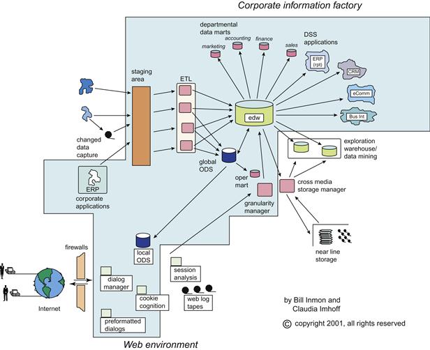
1. Information factory is a widely popular model conceived and designed by Bill Inmon. It uses a data modeling approach aligned with the third normal form where the data is acquired at its closest form to the source, and subsequent layers are added to the architecture to support analytics, reporting, and other requirements.
2. BUS architecture, also known as the Kimball architecture, is based on a set of tightly integrated datamarts that are based on a dimensional data model approach. The data model allows business to define and build datamarts for each line of business and then link the diverse datamarts by aligning the common set of dimensions.
In the information factory architecture shown in Figure 6.4, the data warehouse is built in a top-down model, starting with multiple source systems across the enterprise sending data to the centralized data warehouse, where a staging area collects the data, and the data quality and cleansing rules are applied. The preprocessed data is finally transformed and loaded to the data warehouse. The third normal form of the data model enables storing the data with minimal transformations in to the data warehouse. After loading the data warehouse, depending on the needs of the business intelligence and analytical applications, there are several virtual layers built with views and aggregate tables that can be accessed by the applications. In most cases, a separate datamart is deployed to create further data transformations.
The datamart BUS architecture shown in Figure 6.5 builds a data warehouse from the bottom up. In this technique, we build multiple datamarts oriented per subject and join them together using the common BUS. The BUS is the most common data elements that are shared across the datamarts. For example, customer data is used in sales and call center areas; there will be two distinct datamarts—one for sales and one for call center. Using the BUS architecture we can create a data warehouse by consolidating the datamarts in a virtual layer. In this architecture the datamarts are based on a dimensional model of dimensions and facts.

Pros and cons of information factory approach
Pros and cons of datamart BUS architecture approach
• Faster implementation of multiple manageable modules.
• Simple design at the datamart level.
• Incremental approach to build most important or complex datamarts first.
• Can deploy in smaller footprint of infrastructure.
• A datamart cannot see outside of its subject area of focus.
• Redundant data architecture can become expensive.
• Needs all requirements to be completed before the start of the project.
• Difficult to manage operational workflows for complex business intelligence.
As we can see from this section, neither architecture is completely good or bad. There have been mixes of both these architectures in the current world of data warehousing for creating and deploying solutions. An important aspect to note here is the shared-everything architecture is an impediment irrespective of whether you design a top-down or bottom-up architecture.
The challenges of a data warehouse can be categorized into the following:
• Dependence on RDBMS. The relational model restricts the ability to create flexible architectures. Enforcing relationships and integrity is needed to keep the quality of the data warehouse, but there is no rule that mandates this as a precursor to build a data warehouse.
• Shared-everything architecture. Except for Teradata, all the other databases are built on the shared-everything architecture.
• Explosive growth of data—new data types, volumes, and processing requirements.
• Explosive growth of complexity in querying.
• Evolving performance and scalability demands.
• Unpredictable dynamic workloads.
• User evolution from static report consumers to interactive analytical explorers.
• Data management limitations with sharding (partitioning in the database speak of RDBMS).
While the data warehouse 1.0 has been useful and successful, it cannot meet the demands of the user and data needs in the structured data world. If we were to create the Big Data processing architecture on this foundation, it is not feasible or conducive based on the challenges that have been outlined.
Data warehouse 2.0
The second generation of data warehouses has been designed on more scalable and flexible architecture models, yet in compliance with Codd’s rules. With the emergence of alternative technology approaches, including the data warehouse appliance, columnar databases, and the creation of useful hub-and-spoke architectures, limitations of the first-generation architecture have been scaled back but have not completely gone away.
One of the key aspects of the second generation of the data warehouse is the classification of the data life cycle to create a scalable data architecture as proposed by Bill Inmon in Inmon’s DW 2.0.2 Another proposed solution is the DSS 2.0 data architecture described by Claudia Imhoff and Colin White.3
Overview of Inmon’s DW 2.0
The first-generation data warehouse challenges prompted a newer architecture for the next generation of the data warehouse. The architecture of DW 2.0 has to address three distinct components:
• Data architecture—based on information life cycle.
• Infrastructure—based on data architecture and life cycle.
• Unstructured data—new content of text, images, emails, and more.
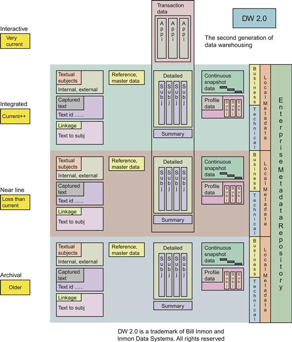
Figure 6.6 describes the architecture approach of Inmon’s DW 2.0. Based on this architecture and foundational elements that it addresses, let us examine the following differentiators in this architecture:
• Data is divided into four distinct layers, based on the type of data and the business requirements for the data. This concept is similar to information life-cycle management, but extends the metadata layer associated with data across the following different layers:
• Interactive sector—very current data (e.g., transaction data).
• Integrated sector—integrated data (e.g., current data that is relative to the business needs, including hourly, daily, or near real time).
• Near line sector—integrated history (e.g., data older than three to five years from the integrated sector).
• Archival sector—archived data from near line.
• Metadata is stored in each layer.
• Each layer has a corresponding unstructured data component.
• Each layer can be created on different platforms as metadata unites the layers.
• Data can be integrated across all the layers with metadata.
• Lower cost compared to DW 1.0.
• Lower maintenance compared to DW 1.0.
The architecture is relatively new (about five years) and is gaining attention with the focus on Big Data.
Overview of DSS 2.0
Another concept that has been proposed by Claudia Imhoff and Colin White is the DSS 2.0 or the extended data warehouse architecture shown in Figure 6.7.
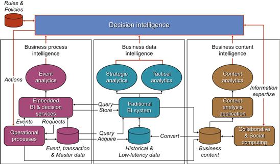
Figure 6.7 DSS 2.0 architecture. Source:www.beyenetwork.com.
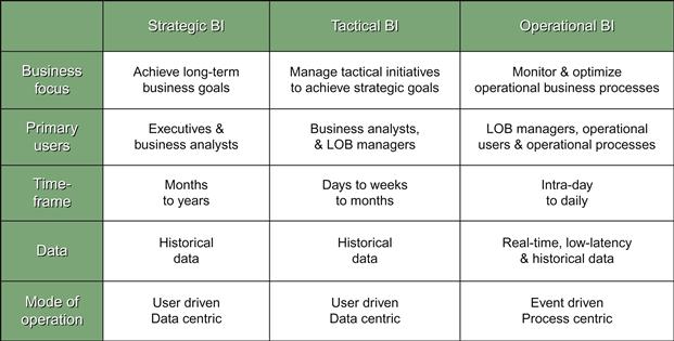
In the DSS 2.0 model, the authors have suggested compartmentalizing the workload of the operational and analytical business intelligence (BI) and adding the content analytics as a separate module. The three different modules can be harnessed using corporate business rules deployed through a decision support integration platform called decision intelligence. The matrix in Figure 6.8 explains the different types of business intelligence needs that can be addressed by the DSS 2.0 approach. The authors explain in the matrix the different types of users, their data needs, and the complexity of processing, and introduce the concept of managing user expectations by understanding their query behaviors.
DSS 2.0 is implemented more from the front-end solution with common metadata integration points in the industry today.
The challenge that faces data warehousing today is not the volume of data alone; the data types and data formats are issues that threaten to violate the data processing rules of the data warehouse. The rules that were designed for relational data cannot be enforced on text, images, video, machine-generated data, and sensor data. The future data warehouse will also need to handle complex event processing and streaming data and support object-oriented or Service Oriented Architecture (SOA) structures as part of data processing.
The future evolution of data warehousing will be an integration of different data types and their usage, which will be measured as the workload executed on the data warehouse. The next generation of the data warehouse design technique will be the workload-driven data warehouse, where the fundamental definition of the data warehouse remains as defined by the founding fathers, but the architecture and the structure of this data warehouse transcends into heterogeneous combinations of data and infrastructure architectures that are based on the underlying workloads.
While Inmon’s DW 2.0 and DSS 2.0 architectures provide foundational platforms and approaches for the next-generation data warehouse, they focus on usability and scalability from a user perspective. The workload-driven data warehousing architecture is based on functionality and infrastructure scalability, where we can compartmentalize the workloads into discrete architectures. In a sense, the workload-driven architecture can be considered as a combination of Inmon’s DW 2.0 and Google’s Spanner architecture.
Summary
As we conclude this chapter, readers need to understand the primary goals of a data warehouse will never change, and the need to have an enterprise repository of truth will remain as a constant. However, the advances in technology and the commoditization of infrastructure now provide the opportunity to build systems that can integrate all the data in the enterprise in a true sense, providing a holistic view of the behavior of the business, its customers, and competition, and much more decision-making insights to the business users.
Chapter 7 will focus on providing you with more details regarding workload-driven architecture and the fundamental challenges that can be addressed in this architecture along with the scalability and extensibility benefits of this approach.
Further reading
1. In: http://www.kimballgroup.com/.
2. In: http://www.bitpipe.com/tlist/Data-Warehouses.html.
3. In: http://ist.mit.edu/warehouse.
4. In: http://tdwi.org/.
5. In: http://www.b-eye-network.com/.
6. In: http://research.itpro.co.uk/technology/data_management/data_warehousing.
7. In: http://www.ithound.com/browse/business-management/business-intelligence/data-mining.
8. In: http://www.teradata.com/resources.aspx?TaxonomyID=3534.
10. In: www.gartner.com.
11. In: www.microsoft.com.
12. In: www.oracle.com.
13. In: www.emc.com.
1Codd, E. F. (1970). A Relational Model of Data for Large Shared Data Banks. Communications of the ACM, 13(6), 377–387. doi:10.1145/362384.362685.
2http://www.inmoncif.com/home/
3DSS 2.0 -http://www.b-eye-network.com/view/8385.