9
Quanta and Optical Spectra
9.1 The Dual Nature of Light–Particles and Waves
In the first few chapters, we studied the various properties of light such as propagation, reflection, refraction, interference, diffraction, and polarization. These topics concentrated on the wave nature of light. All of these phenomena can be explained using classical physics. In this chapter, we will begin our study of the production of light by studying the basic structure of matter. As discussed in Chapter 3, Maxwell’s equations treat the propagation of light, whereas the quantum theory describes the interaction of radiation and matter. The electron plays an important role in this interaction. A combined theory called quantum electrodynamics best describes the modern view of light phenomena by stressing the wave and particle nature of light. As you may have guessed by now, waves and particles have very little in common. Nothing in our human experience can be used to describe a phenomenon that has both a wave and a particle nature. This accounts for the confusion in this area of study. The physicist, Richard Feynman, summed it up beautifully when he described this dual nature of light by saying, “the paradox is only a conflict between reality and your feeling of what reality ought to be.”
9.2 The Discovery of The Electron
Before the late nineteenth century, the atom was thought to be the smallest building block of matter. But, by the end of that century, there was some evidence that the atom could be made of still smaller particles. This evidence was obtained by J.J. Thomson in 1897 with the discovery of the first subatomic particle, the electron. He is generally credited for this discovery, but many other scientists were also involved in similar work at the time.
Thomson’s experiment involved the use of a special glass vacuum tube. He used high voltage electrodes on both ends of this tube. One electrode was charged negatively (called the cathode) and the other one was charged positively (called the anode). Thomson noticed that when he applied a high voltage to the electrodes, the tube walls glowed with a greenish fluorescence.
He later made more refinements to this vacuum tube, such as the addition of a special screen at the end to make observations easier. Thomson discovered that this green glow originated from the negative lead by traveling in a straight line. He subsequently called this phenomenon “cathode rays.” These cathode rays were invisible to the naked eye unless they interacted with another substance such as the glass walls or the special screen at the end of the vacuum tube.
One important result from this experiment was that cathode ray particles are much lighter than normal atoms. This conclusion was brought about after much experimentation with changing the gas type and cathode material in the tube. These changes did not affect the characteristics of the cathode ray particles. He also used a magnet near the trajectory of these particles and noticed that the straight line motion was disturbed by the field. From the effect the magnet had on the particles, he proposed that these particles contained a charge.
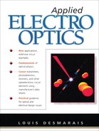
With this information, he refined his design for a more interesting experiment. He added two flat parallel metal plates separated by 1.5 cm. A voltage was applied to these plates creating an electric field between them. He used the magnet again to deflect the cathode rays. Figure 9.1 shows the details of his design. The cathode rays passed through the two plates, and then through the field of the magnet. The two forces involved here could be used to deflect the straight line motion of the cathode ray particles. For example, the deflection could be controlled by varying the plate voltage.
With the experimental design described in Figure 9.1, Thomson was able to determine a parameter called the charge-to-mass ratio (e/m) of the electron. To explain his experiment in more detail, we must first consider the forces involved. The first force occurred between the parallel plates when a high voltage was applied. They were positioned such that the cathode ray beam experienced a downward force due to the electric field there. The second force was due to the magnet. It was positioned such that its force was exerted upward. Since it was already determined that these particles possess charge, they will be affected by both the electric and magnetic fields. The amount of force needed to deflect these particles depends upon the amount of charge present. We must also remember that the particles have a certain forward velocity through both fields. In his famous experiment, Thomson adjusted both the electric and magnetic fields to certain values so that no deflection occurred. Under these conditions, the two forces resulted in a net zero force. As we know from basic physics, the mathematical expression for the two forces here are as follows:
Figure 9.1 J.J. Thomson’s design for measuring charge-to-mass ratio.
F = eE (Electric force) and F = evB (Magnetic force)
We can now present the mathematical expression describing the state when the two forces resulted in a net zero force. In this case, both forces are equal. Thus:
evB = eE
In the above expression, e is the electron charge, v is the velocity of the electron, B is the magnetic field, and E is the electric field. Reducing this expression we get:
E = vB
Since the particles display a motion similar to that of a projectile fired horizontally in the earth’s gravitational field, the vertical displacement or deflection, y, of the electron can be expressed as:
![]()
From Newton’s second law, we know that F = ma or a = F/m. If we use the mathematical expression for the force caused by the electric field, F = eE, we can continue further with our derivation:
![]()
In this expression, L is the distance traveled by the cathode rays. Rearranging terms we get the desired result:
![]()
Thomson obtained 1.6 × 10¹¹ C/kg for this ratio. This result agrees closely with the modern accepted value of 1.7589 × 10¹¹ C/kg. When he used different gases in the tube with different cathode metals, he obtained the same result. This means that the cathode ray particles were common to all metals.
Thomson was able to obtain only the charge-to-mass ratio itself. To find the value for either e or m, one of these must be known. At the time of Thomson’s experiment, it was not possible to perform an experiment to determine either value. Then, in 1912, the American physicist Robert A. Millikan measured the charge on the electron successfully by using his oil drop apparatus. Knowing the value for the electron charge meant that the electron mass could now be determined. We will discuss this experiment later in this chapter.
Before Millikan’s experiment, various attempts were made to determine the charge on the electron. These attempts gave only approximate results. There were disagreements among the physicists at that time relative to the value of the electron charge. Some physicists argued that if all electrons in Thomson’s experiment displayed the same e/m ratio, that did not necessarily mean that they had the same charge. Also, up until this point in time, there was no proof that all electrons were identical.
Example 9.1
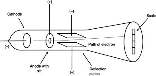
Let us now consider an example using J.J. Thomson’s design as detailed in Figure 9.1. The following physical parameters will apply in this example: the two plates are 5.0 cm long with a separation of 1.5 cm. (a) If these plates are kept at a potential of 60 volts, find the resulting deflection of electrons as they travel the 5 cm path between the plates. The electrons have a kinetic energy of 2500 eV. (b) This deflection can be balanced by applying a magnetic field as described in Thomson’s experiment. Find the strength of the magnetic field necessary to cause no deflection of the electrons.
(a) Looking at the equation developed for vertical displacement, y, we find that we are lacking two variables to solve this problem. These variables are the electric field, E, and the velocity, v, of the electrons. We will find each of these variables from the given information.
The electric field, E, between the plates can be found from the applied voltage and the separation distance. Thus:
E = V/L = 60/1.5 × 10−2 = 4.0 × 10³ volts/meter
The velocity of the electron can be found from the kinetic energy where K.E. = (1/2) mv2. When we rearrange the terms, we get:
![]()
Now, we can substitute the values directly into the equation:
(b) For the condition of no deflection with applied electric and magnetic fields, the following equation can be used:
evB = eE or B = E/v
Solving for B we get:
B = 4 × 10³/2.96 × 107 = 1.35 × 10⁻⁴ weber/meter2
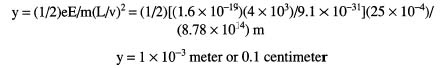
We now continue with our historical development by considering the Millikan oil drop experiment, one of the classic physics experiments. In this experiment, Millikan determined the charge on the electron in units of coulombs. His apparatus used charged parallel plates placed inside of a metal box. The top plate had a small hole in the center. The metal box allowed the environmental conditions inside to be controlled. When a voltage was applied across these parallel plates, an electric field was produced between the plates. Using a special microscope, it was possible to view a portion of the volume of air between the plates. Figure 9.2 shows the details of this apparatus.
In his experiment, a light oil mist was introduced into the volume above the parallel plates. The force of gravity caused these oil drops to fall onto the top plate. Since this plate contained a small hole, eventually an oil drop made it through the opening. With no voltage applied across the parallel plates, the oil drop fell with a terminal velocity determined by the weight of the drop and air resistance. With the application of a voltage to the plates, the descent or rise of the drop could be controlled. Millikan could slow it down, make it stationary, or make it rise back to the top.
The control of the oil drop’s motion could only be possible if it had an electric charge on it. In this case, the electric field between the plates would exert a force on the drop to counter the gravitational force. Using x-rays, he could add one or more charges onto the oil drop and observe its change in downward velocity. By varying the electric field between the plates, he found that the field strength was related to the charge on the oil drop. After observing thousands of oil drops, he came to two very important conclusions:
1. The value for the charge on the oil drop never fell below a minimum amount.
2. The measured charge always came out to a whole number multiple of this minimum value.
From this, Millikan assumed that this minimum charge on the oil drop was due to only one electron. He found the value for e to be 1.591 × 10⁻¹⁹ C. Today, the accepted value for the electron charge is 1.6021 × 10⁻¹⁹ C. Now, with this value, we can calculate the mass of the electron using J.J. Thomson’s result. We show this calculation below:
This result showed a very important characteristic about the amount of electric charge present. Electric charge is not continuously variable in nature but occurs only in discrete amounts. Most scientists at that time did not seem very surprised at this finding. They saw this quantization of electric charge to be very similar to the discrete nature of matter proposed by Dalton and Avogadro. In the last chapter, we saw further evidence for this discreteness with the quantization of light energy and the discrete energy states of atoms.
The electron was eventually accepted as a fundamental building block of the atom. However, the scientists at the time were not sure just how this electron integrated into the overall atomic structure. This acceptance also left the question of charge distribution within the atom unanswered. For the atom to be electrically neutral (no net charge), it must also contain the same magnitude of positive charge. How these charges were distributed still remained a mystery at that time. There were a number of theories proposed by scientists to help explain the electron’s role in the atomic structure.
One of the most popular theories about atomic structure was called the “plum pudding” model for which J.J. Thomson supported. In this theory, the positive charges were distributed evenly within a spherical volume. The newly discovered electrons were thought to oscillate about fixed centers inside this volume. Ernest Rutherford, a well-known scientist at the time, wanted to test the validity of this and some of the other theories. He eventually initiated a research study to look at the basic structure of the atom.
Figure 9.2 Millikan oil-drop apparatus
9.3 The Theory of Atomic Spectra
In 1911, Ernest Rutherford conducted experiments that eventually led to the discovery that a typical atom is composed of a relatively heavy nucleus around which much lighter electrons travel. This nucleus has a positive charge while the electrons have a negative charge. A stable atom will have just enough electrons in number (charges) to balance off the positive charges in the nucleus. He arrived at this conclusion after very close examination of his test data.
Figure 9.3 shows Rutherford’s design for the above experiments. He used a radioactive source of polonium contained in a lead box to generate the alpha particles. The alpha particle is basically a helium nucleus. It is composed of two protons and two neutrons. This configuration results in a net positive charge of +2. Traveling with a velocity of 1.6 × 10⁷ meters per second, these particles acted as subatomic bullets aimed at a thin gold foil of thickness 10−7 meter. Since their mass, charge, and velocity were known, he could determine important parameters about the gold nucleus from this interaction. Fluorescent screens were placed, as shown, to display the locations where the alpha particles ended up after interacting with the gold atoms. After many hours of observations, he came up with some unexpected results. Most of the particles passed straight through the foil to the fluorescent screen on the other side. For this to occur, he reasoned that the gold atoms must have spaces between them. A few of the particles were deflected from the foil by angles that varied from a few degrees to 180°. The few particles that were deflected at large angles caused a problem for the atomic theory at the time.
In the early 1900s, physicists thought that the positive charge of the atom was spread out to a radius of about 10−10 meter. The electrons were also thought to move about inside this volume. With this view in mind, Rutherford could not explain how a massive alpha particle could be deflected by 180° due to the tiny electrons inside the atom. The mass of the electron was known to be much less than that of an alpha particle. Rutherford was later quoted as saying, “It was quite the most incredible event that has happened to me in my life. It was almost as incredible as if you fired a 15-inch shell at a piece of tissue paper and it came back and hit you.”
Figure 9.3 Rutherford’s experiment used to discover a dense atomic nucleus. Notice that most of the alpha particles passed straight through the gold foil.
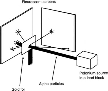
The solution to the problem required a new model for the atom. Rutherford proposed that the electrons moved around the outside of the nucleus instead of inside of it. As for the positive charges, his model had them confined to a smaller radius of about 10−14 meter. Using this model, Rutherford could now explain the observations from his experiments. The number of alpha particles passing through the foil compared with the number that rebounded gave him a clue as to the size of the atomic nucleus. It was found that one out of every 8000 alpha particles were deflected by more than 90°. This deflection resulted when the alpha particle passed through a region of enormous field strength found at the surface of the nucleus. This field results from the positive charges (protons) being confined to such a small volume (the nucleus). Returning back to Figure 9.3, we can see the path taken by the alpha particles as they move through the gold foil. There are a few grazing angles but most of the alpha particles go straight through the foil. Since the nucleus has a net positive charge, the force on the alpha particle will be repulsive. The few particles that were deflected experienced the repulsive force of the gold nucleus.
Now let’s look at the physics involved with the force between charged particles. As we know, these charges exert forces on each other. If e1 and e2 are both electric charges separated by a distance r, the force that each charge exerts on the other charge in a vacuum is given by Coulomb’s law:
![]()
The coulomb force is given in Newtons when using the MKS system. The unit of charge is the coulomb, and the distance between charges is measured in meters. If there are like charges, the force is repulsive. The force is attractive if these charges are unlike.
Next, let’s compare the motion of the electron around its nucleus to that of the earth around the sun. Classical physics says that the electron does not fall into the nucleus of an atom because it is orbiting at a fast enough speed. Coulomb’s equation above shows the same inverse square relationship with distance that characterizes the gravitational force. If classical physics were correct, the electron should move in a similar fashion to an orbiting gravitational mass. Nevertheless, it turns out that there is another condition that classical physics cannot explain. While the electron is orbiting its nucleus, it is constantly being accelerated toward it. According to classical physics, an accelerating electric charge should radiate energy. This means that the orbiting electron should be constantly losing energy due to this emission of radiation during acceleration. The energy loss should eventually cause the electron to spiral into the nucleus. In fact, calculations using classical mechanics predict that the electron should achieve this state in about 10−6 sec. This situation is not observed in a stable atom. How then can we explain the motion of the electron around the nucleus?
Neils Bohr studied the atomic structure by applying classical physics as far as he could. He had to make additional assumptions where necessary to help explain observed phenomena. It was his conclusion that you could not deduce stable positions for the electron by using classical mechanics or electrodynamics. Bohr eventually came up with an empirical model for the hydrogen atom which is applicable to other systems as well. This model will be used later to study the physics involved with optoelectronic devices.
In the last chapter, we discussed the fact that the energy associated with an electron orbiting an atom can be exchanged only in discrete amounts called quanta. Neils Bohr did his famous work on this subject. He was primarily interested in finding a theoretical basis for explaining the spectral or emission lines of hydrogen. He noticed a series of bright lines when the light emitted from excited hydrogen gas was passed through a device called a spectroscope. These bright lines, he reasoned, are a characteristic of a particular atom or molecule. Thus, hydrogen will be different from oxygen in the number and positions of these emission lines. Hydrogen also has the simplest emission spectrum.
To explain why hydrogen atoms emit only discrete characteristic frequencies, Bohr proposed two assumptions or postulates:
1. Electrons can occupy only certain discrete quantized orbits or stationary states of fixed energy. These particular stable orbits or states are nonradiating and obey both Coulomb’s and Newton’s laws. This means that the angular momentum of each orbit must also be fixed. The lowest or normal state is known as the ground state.
2. When an electron changes from one stationary state to another, the energy emitted or absorbed equals the difference in energy between the two states. The frequency, v, of this radiation can then be determined by the formula
![]()
where ΔE is the difference between the two energy states and h is Planck’s constant. Thus, the energy difference from a higher energy level to a lower energy level can be written as ΔE = En2 − Enl.
This emitted or absorbed energy involves the exchange of photons. The photon’s energy is the difference between these two energy states. Thus, each particular emission line in the hydrogen spectrum corresponds to the emission of photons with a particular energy given by the above equation.
Bohr came to the conclusion that the classical mechanical interpretation of the atomic system required modification. We have already seen two instances where this was done. Planck’s blackbody radiation theory and Einstein’s photoelectric effect required modifications from the classical view. Thus, Bohr assumed that there were only certain electron orbits that did not result in the emission of energy. If electrons stayed in these orbits, the energy remained fixed. When electrons changed from one orbit to another, an exchange of energy was involved. This also meant that the angular momentum of an electron in one of these fixed energy orbits is quantized. An expression for the angular momentum in this case is given below:
In this expression, L is the angular momentum, n is the particular state of the electron, me is the mass of the electron with velocity, v, in a circular orbit of radius, r. Now, we will apply Coulomb’s law in this case. When we make the Coulomb force equal to the centripetal force of the electron, we get the following equality (the electron has a charge of −e, the proton has a charge of +e):
![]()
Next, we substitute for velocity, v, using the formula mvr = nh/2π. After rearranging terms and simplifying, we get an expression for the allowed radii of the Bohr atom:
![]()
where rb is the first Bohr radius (n = 1). The various orbits can then have the following values, rb, 4rb, 9rb, and so forth. Solving for rb, we get the actual length of this radius:
rb = 5.292 × 10⁻¹¹ meter
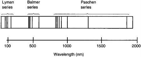
Close examination of the hydrogen emission lines showed that there are at least three different series or sets of these lines. The first series were discovered by Johann Balmer in 1885. This particular series of emission lines can be found in the visible part of the spectrum. Figure 9.4, a sketch of a spectrograph for hydrogen, shows the three different series of hydrogen emission lines and their location in the spectrum. For the Balmer series, three bright lines can easily be seen through a simple spectroscope while viewing a hydrogen discharge tube. The hydrogen alpha line is located at 656.3 nm (6563 Angstroms). The hydrogen beta line is at 486.1 nm (4861 Angstroms), and the hydrogen gamma line is at 434.0 nm (4340 Angstroms). As you can see, another series of lines is located in the infrared region and one more is located in the ultraviolet region of the electro-magnetic spectrum.
Figure 9.4 Spectrograph of hydrogen showing the first three series of emission lines.
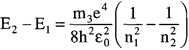
To explain the formation of these lines, Bohr reasoned that there are only a finite number of allowable stable orbits that an electron can occupy around the nucleus. Each orbit has a different energy associated with it given by the following equation:
![]()
En is the energy associated with the formation of a stable orbit. The mass of the electron is me, e is the electron charge, and ε0 is the vacuum permittivity. In the above formula, n is an integer or quantum number. When n = 1, this is the lowest allowed orbit for the Bohr hydrogen atom. Solving the above equation for the condition when n = 1, we get E = −13.5 electron volts (eV). The negative sign means that the energy given applies to a bound state for the electron. In this case, an excess of 13.5 eV must be applied to this system for the electron to break free of the nucleus. If this happens, an ion will be formed because the lost negative charge of the electron leaves a net positive charge of the nucleus (one proton). This energy is also referred to as the ionization energy.
The energy emitted by an electron as it falls or jumps from a higher level to a lower level orbit can then be defined as:
The energy released is then given by the following expression where ν is the frequency of the emitted photon:
ΔE = En2 − Enl = hν
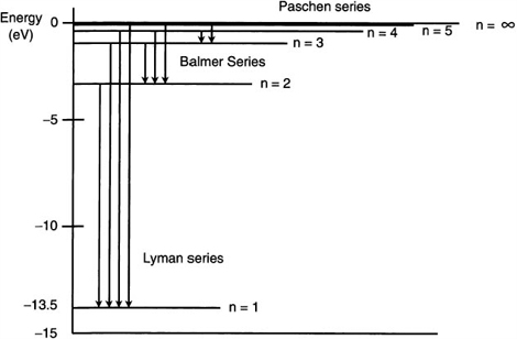
A transition diagram for hydrogen is given in Figure 9.5. The various energy levels for the allowed orbits are represented by horizontal lines. These transitions correspond to the vertical arrows and show up as emission lines. This diagram shows the energy transitions for the Lyman, Balmer, and Paschen series. Each series has a common lower energy level. The spectral lines are obtained by the various combinations of integers for n1 and n2. The energy associated with each line can be calculated by using the above formula. As stated previously, the Balmer series of spectral lines were the first to be discovered. When Johann Balmer was presented with the observations of the four visible emission lines of hydrogen, he was able to come up with the portion of the formula contained in the brackets. Balmer had an interest in solving numerical puzzles, so he tried various numerical combinations. By setting the lowest value to n = 2 and then using n = 3, 4, 5 ,6 for the higher levels, he able to match this result with the four observed wavelengths. In the process, he had to treat all of the quantities to the left of the brackets as one constant.
The Bohr model of the hydrogen atom had at least one serious problem, but it does give essentially correct numerical results. In the Bohr model, electrons move around the nucleus in fixed, stable orbits. This is impossible according to classical physics because a charged particle, such as an electron, moving in an electrostatic field should radiate energy. As this energy radiates from the charged particle, its energy level should gradually decrease, causing a smaller orbital radius. This means the electron should, according to classical physics, eventually fall into the nucleus of the atom. The Bohr theory was eventually superseded by the modern quantum theory to explain this discrepancy. The quantum theory uses wave or state functions to describe the atomic system. A study of these wave functions is beyond the scope of this book. Let us next consider an example using Bohr’s model of the hydrogen atom.
Figure 9.5 Energy level diagram for hydrogen showing a few transitions in each series.
Example 9.2
Looking at the diagram in Figure 9.5, we see the Balmer series of emission lines for hydrogen. Find the wavelength of the emitted photon as an electron makes a transition from the energy state at n = 4 to n = 2.
To solve for the wavelength of the photon, we must first find its energy. Then, from its energy, we can determine its wavelength using the Planck relationship:
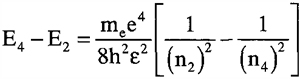
When we substitute the values into the right side of the equation, we find:
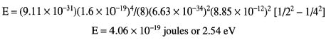
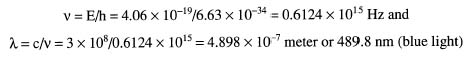
Now, since E = hν, we can now solve for the wavelength by finding the frequency:
9.4 Electron Waves
In 1924, Louis de Broglie predicted the existence of matter waves. He proposed that this wave-particle nature of light could also apply to any particle. The relationship that he came up with represents a direct violation of the classical view. That is, an electron acts as a wave phenomenon. He used the expressions below to prove his theory:
![]()
and
E = hν = pc
In both expressions, p is the momentum of the particle of matter. The dual nature of light can be described using the above two equations. Each equation contains a variable for the wave concept (λ and ν) and the particle concept (p and E). According to deBroglie, this relationship should hold true for any particle having a linear momentum, p. Looking at this relationship, we can see that as a particle’s momentum increases, its wavelength will decrease. Since h is a very small number, this dual wave-particle nature of matter becomes apparent only in the microscopic realm of atoms and subatomic particles. And, it is probably a good thing that h is very small. Imagine what this world would be like if Planck’s constant were significantly larger than it is now! With the value of h as it is, electron size particles should display wave properties such as diffraction, but macroscopic objects, such as baseballs, should display properties of a particle. About three years after deBroglie proposed this relationship, the wavelike nature of the electron was displayed by an electron beam.
In 1927, C. J. Davisson and L. H. Germer proved that the electron can be described as a wave phenomenon when they obtained diffraction patterns from reflected electrons. Davisson was working on the problems associated with vacuum tubes at AT&T when he noticed the scattering of electrons from a nickel crystal target. With the help of Germer, he researched this effect further by allowing an electron beam to hit this nickel crystal target at normal incidence. They also used a detector sensitive to electrons (an ionization chamber). When they made a plot of scattered electrons versus the angle of collection, they obtained a diffraction pattern with maxima and minima. Applying the deBroglie formula to find the electron wavelength, they found close agreement with the classical diffraction formula, nλ = d sin θ. In this case, the spacing, d, of the atomic planes in the nickel crystal was 2.15 × 10⁻¹⁰ meter. X-ray diffraction studies provided this distance. The angle of diffraction for which a strong maximum occurred was found to be 50 degrees. We solve this expression below:
The atomic planes of the crystal performed like a diffraction grating producing the observed diffraction pattern. This physical design satisfies the Bragg condition that is also observed in many other instances involving other types of electromagnetic radiation. Using the deBroglie wavelength formula, they obtained 1.67 × 10⁻¹⁰ meter (see Example 9.3 for this solution). Thus, there was very close agreement between both methods. Now we see why the wave properties of the electron were not discovered until this time in history. From our earlier discussions on diffraction, recall that the slit width or aperture size must be on the order of the wavelength to observe this effect. When the aperture becomes much larger, the effects of diffraction and interference are not observed. In the above experiment, the spacing provided by the atomic planes met this requirement.
In 1937, Davisson and G.P. Thomson, son of J.J. Thomson, received the Nobel prize for their work that showed the wave nature of electrons. We will next present interesting examples that involve calculating the deBroglie wavelengths for two very different sized objects.
Example 9.3
In Davisson’s experiment described above, he used electrons having an energy of 54 eV. Find the deBroglie wavelength in this case.
Since we know its energy, we can find the electron’s velocity from the kinetic energy formula. We need to calculate its velocity to determine its momentum, p. Thus:
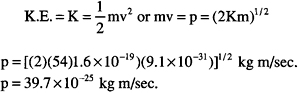
Now, we can use the deBroglie relationship to find the wavelength:
![]()
This result compares very closely to what Davisson found when using the classical diffraction formula and his observations.
Example 9.4
We will next consider an example from the macroscopic world. Find the deBroglie wavelength of a 100 gram golf ball traveling at 30 meters per second.
![]()
This wavelength is extremely small, and for this reason, we do not think of macroscopic-sized objects as having a wave-like nature.
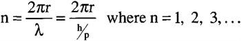
With his wavelength formula and the condition for angular momentum, deBroglie came up with an explanation as to why electrons are only found in certain acceptable orbits around the nucleus. To illustrate this, we use the analogy of a standing sound wave in a long gas-filled tube. We can also use an example of an electromagnetic wave in a wave-guide. In both of these cases, there exists a particular length at which the wave resonates within the cavity producing a standing wave.
Figure 9.6 shows the application of a standing electron wave adjusted in wavelength to fit an integral number of times, n, around the circumference or orbit of the Bohr atom. This concept, while regarded as oversimplified, can be used to help us understand why the electron can occupy only discrete orbits or states. Any other orbit that does not contain an integral number of wavelengths in circumference is not allowed, and thus does not occur. These orbits are also known as stationary states because they have a defined energy level. The mathematical expression for these acceptable orbits can be given as:
Thus, we have seen that electrons and photons possess particle and wave-like natures. This means that they can display normal wave properties such as diffraction and interference. Light phenomena, which we normally think of as wave motion, can also display a particle-like nature. This was shown in our discussion on the photoelectric effect. There is a way to help us understand this dual nature of electromagnetic radiation. When considering the propagation of light, it will behave as a classical wave. When energy exchange is involved, it will behave as a classical particle. However, nothing can behave as a classical wave and a classical particle at the same time.
The exchange of energy using quanta is of primary importance in the study of electro-optics. When using optical sources, photons are generated in the interaction of matter and energy. Semiconductor light sources will be studied in the next chapter. These semiconductor light sources emit photons at a particular energy determined by the relationship, E = hν. The emitted photons behave as particles just before they leave the surface of the source. When they propagate through media such as air, space, or a fiber optic waveguide, wave-like properties apply. Maxwell’s equations can be used to describe the electromagnetic field in this case. Next, as these photons strike the surface of an appropriate optical receiver, we must again consider the particle-like properties of the photon. The process involved here is very much the reverse of the emission process that produced the photons.
Figure 9.6 An electron wave around a Bohr atom. It can fit only an integral number of times around it.
The absorption of a photon by an atom of the receiver material results in an electron of the receiver material becoming excited to a higher energy level. For this to occur, the energy of the incident photon, E = hν, must be equal to that required to excite the electron to a higher level (band gap energy). When the electron is excited to a higher energy level, the conduction properties of the atom are changed and electron flow in the bulk material occurs.
In Section 9.3, we discussed the theory of atomic spectra. We learned that a series of bright emission lines can be seen from excited hydrogen atoms when using a device called a spectroscope. In the next section, we will detail how to construct such a device.
9.5 Low Cost Spectroscope
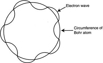
In our previous discussions, we described how photons were produced in the interaction of radiation and matter. A practical optical instrument, the spectroscope, can be used to analyze light to determine what wavelengths or photon energies are involved in this interaction. The spectroscope accomplishes this by dispersing the light into its individual wavelength components. A glass prism or a diffraction grating can be used for this purpose. Our low cost spectroscope will use a diffraction grating in its construction. It is simple to make, and provides for very accurate optical measurements in the visible portion of the spectrum. The description of how to make this spectroscope originally appeared in The Physics Teacher magazine, April 1967, page 173. To make this spectroscope, you will need the following materials:
1. A box measuring approximately 9” long by 6” wide by 2” deep with a removable or hinged cover (A cigar box or video tape box will work nicely)
2. A diffraction grating having 23,000 lines/inch (This can be obtained from Edmund Scientific, part number C40,267)
3. Plastic centimeter ruler
4. 3” × 5” Index card (or an optional slit from Edmund Scientific, part number C39,522)
5. Razor blade
To construct this spectroscope, refer to Figure 9.7.
1. Make a 1” hole in the box centered as shown approximately 1½ inches from the right edge. This hole will be needed to mount the diffraction grating later on in the construction.
Figure 9.7 A low cost spectroscope.
2. Directly opposite the line of sight of this hole, make another hole for the slit. This hole must be about ½” in diameter. It is very important that the center line for the holes line up with the side of the box as shown.
3. To make the slit for the light to enter, cut into the index card with a razor blade. The slit should be about 12 mm long and no more than 1 mm wide. You may need to practice on another piece of paper to get this right. As an option, a mounted slit can be used.
4. After successfully making the slit, trim the index card and tape the slit over the ½” hole. The slit must be oriented vertically and then centered over the hole.
5. Carefully cut a piece of diffraction grating to be placed over the 1” hole. The ruled lines must also be oriented vertically. Use tape to keep it in place.
6. The centimeter ruler must be fastened to the inside of the box as shown. The edge or zero point of this ruler should line up with the slit. This will make future measurements easier.
The operation of the spectroscope can easily be checked by aiming the slit at a light source such as a fluorescent light. When looking into the end with the grating, bright emission lines on a continuous spectrum background can be seen. Other lamps, such as mercury vapor and quartz halogen, should give similar results but with a different set of emission lines. Looking closely at these lines, you can also see the centimeter ruler. We will use this ruler to determine the diffraction angle for a particular emission line. If the diffraction angle and slit spacing are known, we can easily determine the wavelength of the emission line.
As you remember from Chapter 6, the mathematical relationship that we can use in this case is the diffraction formula:
nλ = d sin θ.
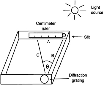
Figure 9.8 Measurement of θ using the spectroscope.
In this equation, n is the order number (one in this case) and d is the spacing between the lines on the grating. To determine the angle θ, we must know the lengths of two sides of the triangle shown in Figure 9.8. Substituting into the above equation for sin θ, we get:
nλ = d sin θ = d A/C
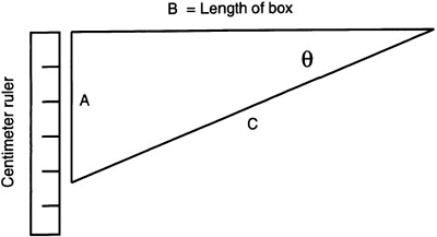
If you use this method to determine the diffraction angle, θ, you will need to make a scale model of the triangle to determine the lengths of A and C. These measurements must be as accurate as possible. An alternate method is to obtain the fixed measurement of side B with the measurement of side A. From these two sides, the diffraction angle can be determined by using the following trigonometric relationship:
tan θ = A/B
Finally, we must determine the spacing, d, from the lines per inch of the diffraction grating. If we convert this measurement to centimeters, our calculations will be easier. We know that 2.54 centimeters equals one inch. Using this information, 23,000 lines/inch of the grating equals 9055 lines/centimeter. The spacing, d, can now be calculated as follows:
d = 1/9055 lines/cm = 1.10 × 10⁻⁴ cm or 1.1 × 10⁻⁶ meter
We are now ready to demonstrate how to determine the wavelength of an emission line from the measured angle of diffraction.
Example 9.5
Using our spectroscope, we find the angular measurements for two particular emission lines. The first one has a measured angle of diffraction of 36°. The second has a measured angle of diffraction of 23.5°. What wavelengths do these emission lines correspond to?
Using the above formula, we get for the first emission line:
![]()
The second emission line can then be calculated as:
![]()
You can see from the above results the accuracy of this instrument due to the relatively large dynamic range available between red and violet wavelengths.
Summary
In this chapter, we have seen the important role that the electron plays in the interaction of radiation and matter. Electrons can occupy only certain discrete quantized orbits or stationary states of fixed energy. This energy is not continuously variable as classical physics would predict. This means that when the electron changes from one orbit or state to another, the energy emitted or absorbed equals the difference between these two states. This is why distinct emission lines can be seen when using a spectroscope to view excited hydrogen atoms. Hydrogen atoms were considered because they are the simplest to use in an explanation for how this energy exchange happens. We will see later that this interaction of radiation and matter also occurs in solid materials.
In the next chapter, we will continue with a discussion of this interaction of radiation and matter as we consider solid materials such as semiconductors. This discussion will involve the particle-like nature of light. We will see why semiconductors make very useful light-emitting materials.