12. Understanding Price Changes
Option prices are in constant movement. So are the values of structured securities that contain options. This chapter looks at the components of option value and the factors that drive changes in those values. The chapter begins with a hypothetical investment, explains the role of implied volatility in constructing an investment profile, and then tracks option prices in terms of intrinsic value, time value, and the elements of extrinsic value. The Greeks are covered in more detail in the next chapter.
Investing in XYZ
Imagine you are watching CNBC’s Mad Money. Jim Cramer just interviewed the CEO of Company XYZ. You already know the company and like what you heard in the interview. You think now is a good time to buy. You have a choice of buying the stock or buying an option on the stock. The option you are considering has a one-year term and a strike price of $95.
The current stock price is $100. The company doesn’t pay a dividend. Assuming a zero interest rate and 30% volatility, the model results in Figure 12.1.

The option price is $14.29 (Cell I5). The model uses the Black-Scholes formula and the pricing assumptions on the display screen. Then assume that you look at a real-time quote from your trading platform, and the quote is $13.50. It is cheap compared to the Black-Scholes value, so you look more closely at the pricing assumptions.
The option term, the stock price, the dividend rate, and the strike price of the option are all known. The only two pricing variables that could be different are the risk-free rate and volatility. For purposes of this example, assume that the risk-free rate is zero and not a source of difference between the two prices. That leaves only volatility.
Using Implied Volatility to Estimate Future Stock Price Distributions
When you price an option using the Black-Scholes formula, you have to specify the volatility assumption. It might be an estimate of volatility based on historical averages or some other estimate that reflects your outlook. The estimate is a pricing assumption. In this case, an assumption of 30% volatility translates into an option price of $14.29. The graph on the display page also reflects the 30% assumption. Whatever volatility you enter in Cell C8 is used to construct the probability distribution and to price the option.
The question now is whether you should adjust your estimate of volatility to reflect the option price of $13.50. That depends on your point of view. Some traders put a lot of effort into developing a volatility estimate. If they have the conviction that 30% is the right number, they might use it for analysis, regardless of the difference in price. They might even decide to buy the option for $13.50 because it is cheap relative to their estimated price of $14.29.
However, when I build structured securities, I am more interested in market information than I am in figuring out whether a particular option is cheap or expensive. That is why, at least as a starting point, I want the investment profile to reflect volatility implied in the option price. So instead of estimating volatility, the investment profile uses implied volatility. Implied volatility is the volatility currently priced into exchange-traded options. Using implied volatility is one way of listening to the market as it tells you what is currently being priced and what that means about possible future stock prices. Of course, you can adjust the volatility to reflect a particular view, but by using implied volatility as a starting point, you will be more consistent with market costs to hedge the position.
How do you know the implied volatility? If you have access to a trading platform or real-time market data that includes implied volatility, it is provided for you. You can also calculate it yourself by trial and error. (There is no easy way to do it by reversing the Black-Scholes formula.)
One way to do this is with Goal Seek, a standard function in Excel. Goal Seek uses an iterative trial-and-error process that zeros in on the right answer. To do this, go to the Black-Scholes add-in or other option pricing page. Click Tools in the Excel menu and select Goal Seek. A box like the one shown in Figure 12.2 appears.
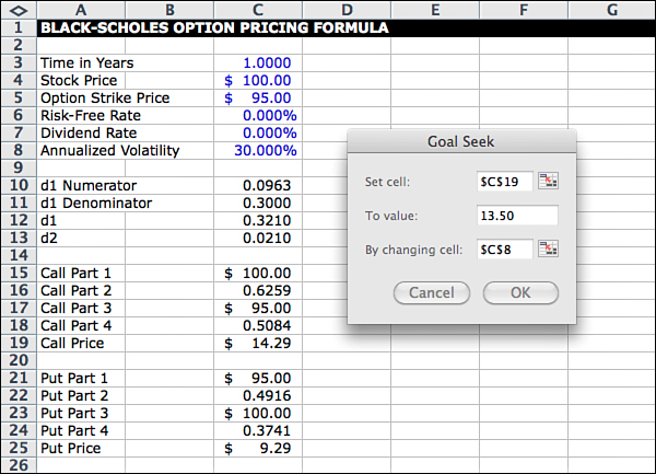
In the Set Cell field, enter the cell location for the option price. In the To Value field, enter the option price you are looking for; in the By Changing Cell field, enter the cell where volatility is entered.
After clicking OK, you see that the answer from Goal Seek is 27.905%, which is the volatility that produces an option price of $13.50. This is the implied volatility that should be used to construct the investment profile so that the probability distribution is consistent with actual option pricing on the exchange. Figure 12.3 shows the new starting point.
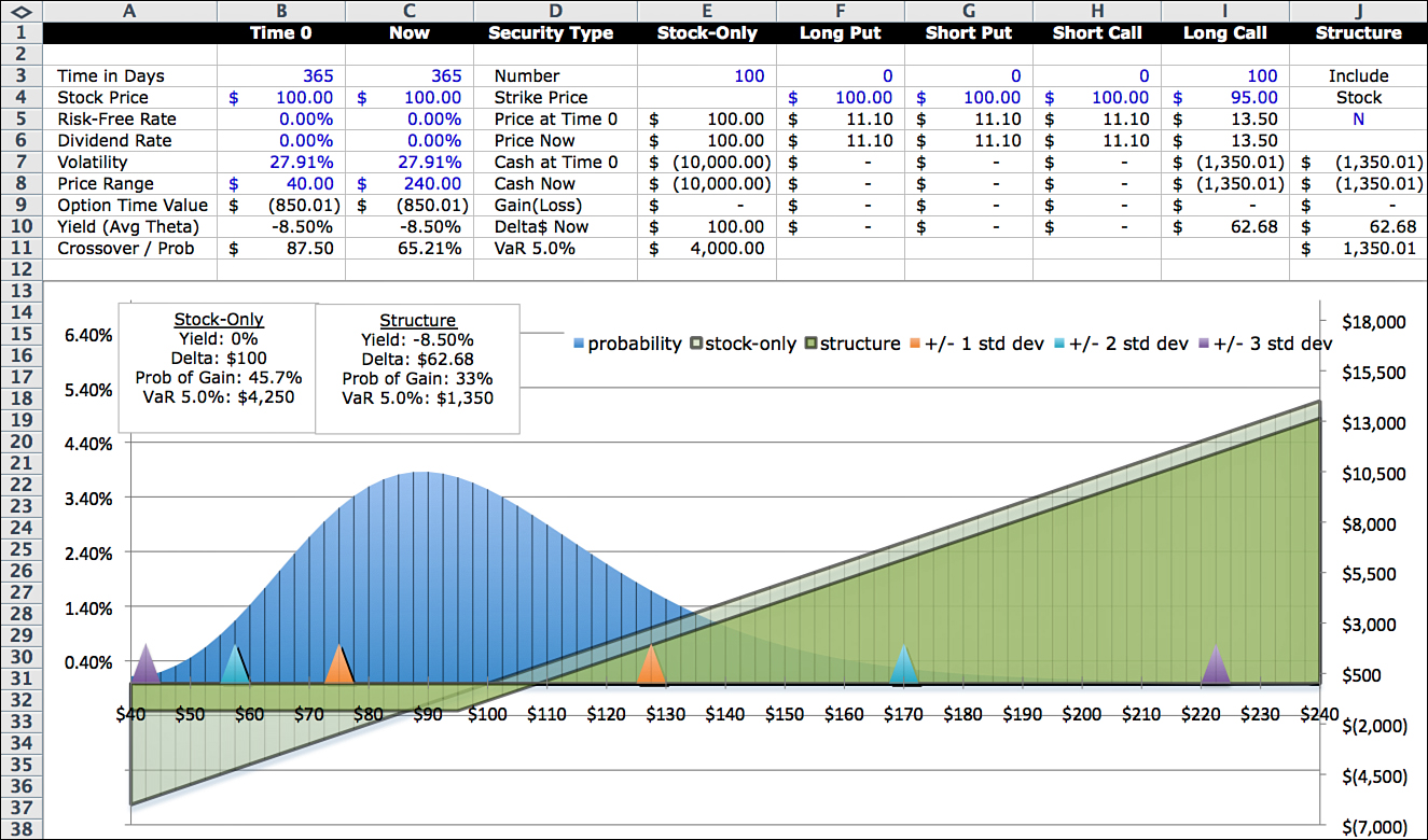
In this implied volatility version, yield is slightly less negative because the option costs less. Delta, the probability of a gain, and VaR are roughly the same as before. Even though the results are similar to those using 30% assumed volatility, this is a more logical starting point for our analysis.
Intrinsic Value, Time Value, and Extrinsic Value
Several terms, including intrinsic value, time value, in-the-money, time decay, time value, time value premium, and extrinsic value, describe components of option value or explain changes in option values. The following definitions are from the Chicago Board Options Exchange website (www.CBOE.com):
• Intrinsic value: The value of an option if it were to expire immediately, with the underlying stock at its current price; the amount by which an option is in-the-money. For call options, this is the difference between the stock price and the striking price, if that difference is a positive number, or zero otherwise. For put options, it is the difference between the strike price and the stock price, if that difference is positive, and zero otherwise.
• In-the-money: A term describing any option that has intrinsic value. A call option is in-the-money if the underlying security is higher than the strike price of the call. A put option is in-the-money if the security is below the strike price.
• Time decay: A term used to describe how the theoretical value of an option “erodes” or reduces with the passage of time. Time decay is especially quantified by theta.
• Time value: The portion of the option premium that is attributable to the amount of time remaining until the expiration of the option contract. Time value is whatever value the option has in addition to its intrinsic value.
• Time value premium: The amount by which an option’s total premium exceeds its intrinsic value.
Although not defined on the CBOE website, extrinsic value is a term generally used to indicate sources of change in value that are not “predictable.”
For our example (dollars are per share):
• The option’s intrinsic value is $5.00.
• The option is “in-the-money.”
• The option will experience time decay.
• The option’s time value is $8.50.
• The option’s time value premium is $8.50.
Because the option contract in the model covers 100 shares, the model displays these per share values times 100.
Example of Two Outcomes
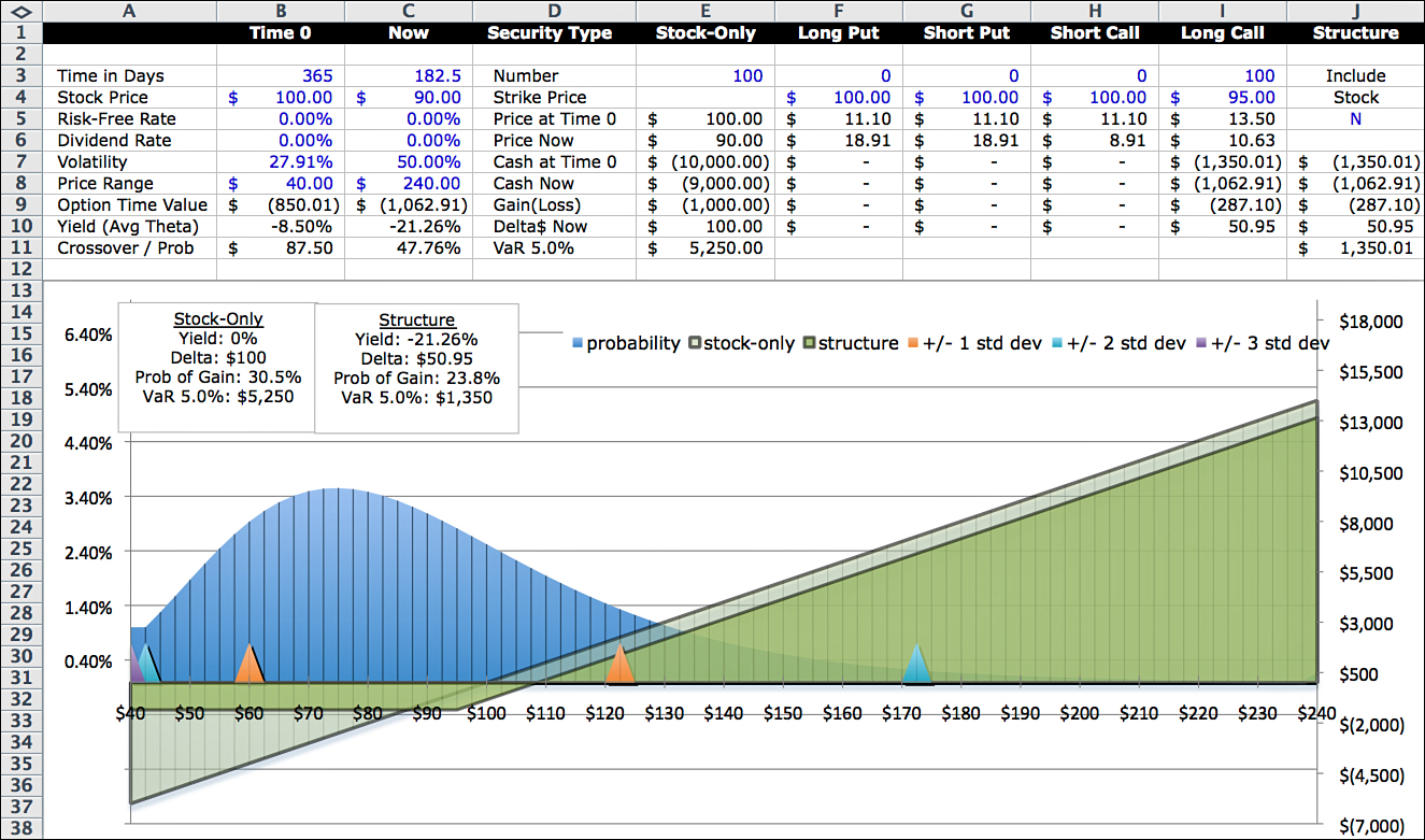
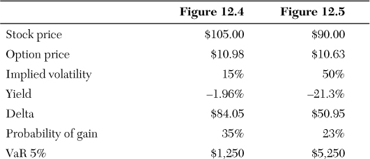
Now let’s run the clock forward six months and consider two different outcomes in Figures 12.4 and 12.5. In the first scenario, the option price on the exchange is $10.98; in the second, the option price is $10.63. The two option prices are close, but the situations and analysis are different. The following summarizes the stock prices, the option prices, and implied volatilities with six months remaining on the option term:
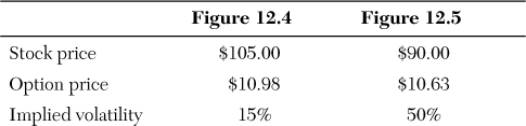
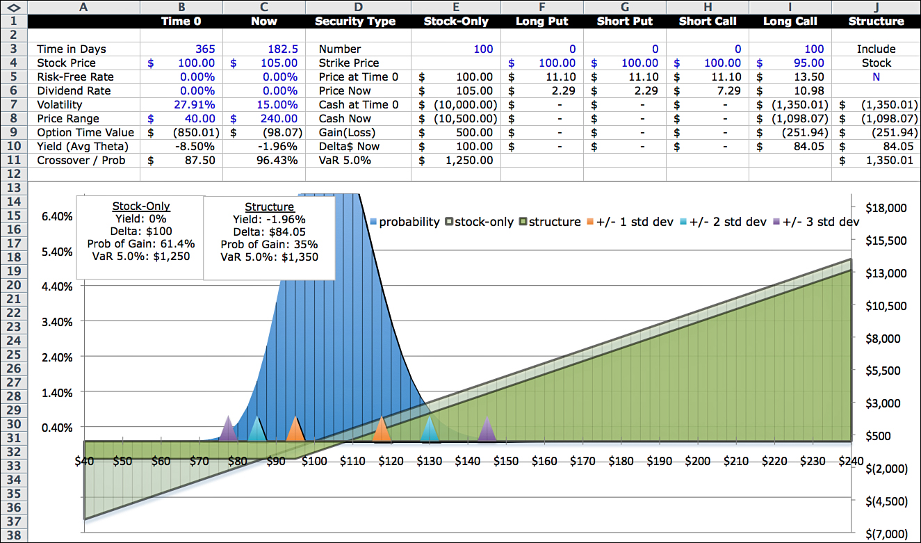
The first scenario is consistent with a calm, up-trending market, where prices increase and volatility decreases to reflect investor optimism. To visualize this market condition, look at the investment profile in Figure 12.4—particularly the center point and the relative spreads of the probability distributions. Compared to Figure 12.3 six months earlier, Figure 12.4 has a narrower profile (reflecting the lower volatility), and the center point of the distribution has moved to the right (reflecting the higher stock price).
In terms of metrics, the yield is less negative because there is less time value; delta is higher because the option is deeper in-the-money. The more an option is in-the-money, the higher the delta. This makes sense because the option begins to approach a dollar-for-dollar move with the stock as the stock price moves above the call’s strike price.
Now look at the second case, where the stock price has moved down and volatility has moved up. These conditions are consistent with a more turbulent market.
Even though the option price is close to the first scenario, the profiles look nothing alike. Neither do the metrics. Now the option is almost all time value because the stock price moved from above to below the strike price. At this point, the option has no intrinsic value and is $5 out-of-the-money. Here is a summary of the two scenarios:
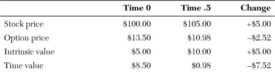
The question now is, how do you analyze these two possible outcomes in terms of intrinsic value and time value? Here is a comparison of intrinsic and time value for the two scenarios:
Scenario 1:
Scenario 2:
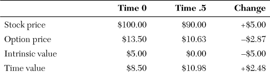
These numbers might be accurate, but how useful are they in explaining what happened? For instance, does knowing that the intrinsic value went up by $5 in the first case and down by $5 in the second case really account for the $15 stock price difference ($105 vs. $90)? And what about time value? In the first case, it declined by $7.52; in the second case, it increased by $2.48. Can time value really increase? That seems to violate the basic notion that time value should decay.
Some experts make a distinction between time value and another metric, extrinsic value, explaining that time decay is a predictable process and should not be confused with or combined with the effects of other pricing variables, such as volatility. For example, Michael Thomsett writes:
Time value by itself is quite predictable and, if it could be isolated, would be easily predicted over the course of time. Simply put, time value tends to change very little with many months to go, but as expiration nears, the rate of decline in time value accelerates and ends up at zero on the day of expiration... Time/volatility value is often described as a single version of “time value premium.” If these two elements are separated, option analysis is much more logical.1
And:
The portion attributed to volatility might be accurately named “extrinsic value.” This is the portion of an option’s OTM premium beyond pure time value. Extrinsic value can be tracked and estimated based on a comparison between option premium trends and stock volatility.
Looking at value in this way, time value increasing by $2.48 doesn’t make sense.
Attribution: Explaining Why the Option Price Changed
It helps to make a distinction here between the components of option value “at a point in time” and the attribution of changes in option value occurring “between two points in time.”
There is nothing wrong with using the terms intrinsic value and time value to talk about the components of an option “at a point in time.” But those terms don’t tell the whole story when looking at changes in option values across time.
Because option prices are determined by six pricing variables, a change in any of those variables affects the price. Of the six, two are fixed after a particular option is chosen: the strike price and the dividend rate. In addition, although the risk-free interest rate can change, it is not a significant contributor to changes in option values, particularly now, with very low market interest rates in effect. So let’s ignore it. That leaves three pricing variables: time, stock price, and volatility.
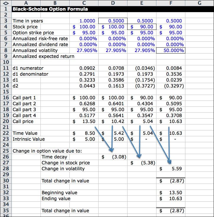
The analysis of changes in option prices should include the effects of these three variables. Look at Figure 12.6. It lays out a procedure for isolating and measuring the effects of the variables. It is the Black-Scholes formula add-in, modified by copying the formula into three additional columns.
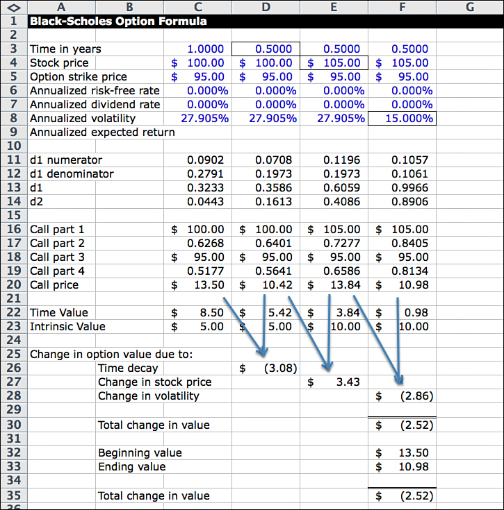
The pricing variables in Column C are the conditions at Time 0 (one-year term, $100 stock price, and 27.905% volatility). The last column shows the conditions after six months (six months remaining, $105 stock price, and 15% volatility).
The two intermediate columns help to isolate the effects of changes. In Column D, the only variable that changes from Column C is time. By comparing the option price in Column D—which assumes both the stock price and the volatility are the same as Time 0 conditions—to Column C, you see the effect of “time alone.” In this case, with the other variables held constant, the change in the option price due to time is the difference in the option price at Time 0 ($13.50) and the option price at Time .5 ($10.42), or a decrease of $3.08. Similarly, the effect of the change in the stock price is the difference between Column E and Column D, or an increase of $3.43. Volatility accounts for a decrease of $2.86.
• Point in time summary: Rows 22 and 23 show the straightforward breakdown of intrinsic and time value across the columns. These numbers are correct; they indicate how much of an option value is in-the-money and how much is not in-the-money. That is all they are intended for. Not that these numbers are not useful—in fact, the model uses time value quite a bit, to give you an idea at “a point in time” how much average yield is possible, assuming that stock prices and volatility remain constant. It is one of the dashboard displays.
• Sources of change analysis: Rows 25–30 show the real story of what happened to the option price and why it changed. The arrows indicate how each component is related to the step-through pricing.
A natural question at this point is whether the two sections can be related by formula. Can you derive Rows 25–30 on the basis of Rows 22–23? That depends. If all you have is the first and last columns, the answer is no. If you have the four columns, it can be done, but it is more confusing than it is worth. To do it, you have to track the excess of the stock price drop over the reduction in intrinsic value. For example, in the second scenario, the drop in stock price is $10. Because intrinsic value started at $5, it can go only to $0. So there is an additional drop in price of $5 below intrinsic value.
The Probability Distribution
It is also possible to visualize the components of change. By running the model iteratively, you can step through the changes in the probability distribution attributable to a particular pricing variable change. For example, if you want to see the effect of time, run the model and change only the time remaining on the option term; keep the stock price and volatility constant. See Figure 12.7.
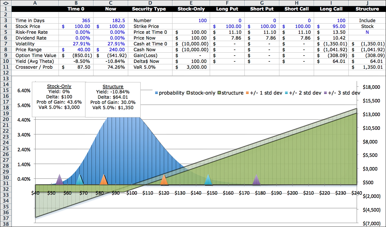
This view enables you to see not only in hindsight why something happened, but also in advance what to expect. For example, when this option was purchased at Time 0, this view will forecast the outcome if nothing changes other than time. Notice that the Gain (Loss) in Cell J9 is a loss of $308.09. Also notice that the probability of a gain in the text boxes dropped from 43.6% to 30.0%. In addition, the rate of time decay accelerated from –8.50% to –10.84%.
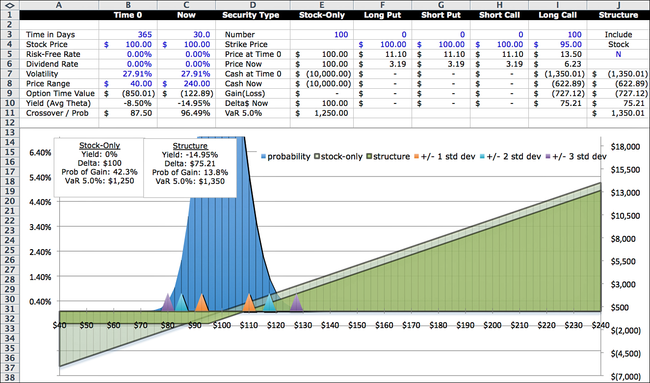
You can continue this process, stepping further out in time. Figure 12.8 is a snapshot with only one month left on the option term. (If you put together a series of snapshots, it creates what I call time lapse photography, a kind of options movie you can create with macros to step through a predefined scenario.)
The Second Scenario: Turbulent Market
Figure 12.9 illustrates the sources of price change for the second scenario, in which the stock price drops to $90 and the volatility increases to 50%.
When the stock price falls significantly below the strike price, the option quickly becomes “disconnected” from the stock, and delta falls quickly as well. In this example, the stock price was only $5 below the strike price. If the stock price were $80, delta would be $37; at $70, delta would be $25.
Time decay in this scenario is the same as before, a decrease of $3.08. This is a reasonable answer. It moves in the right direction and is the same for both examples. As Thomsett pointed out, time value is predictable.
Here is a summary of the changes in value:
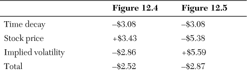
Time decay is the same, but the other two factors are very different, moving in opposite directions. The net effect is that the factors offset each other to a large extent, ending with similar option values.
The Gain (Loss) Analysis Perspective
Why would anyone buy a long call option if they expected the stock price to stay the same? The trade loses money as the time value decays to nothing. You buy a call option if you think the stock is going up. And when you have an opinion about how much you think it is going up, it makes sense to add another step to the analysis.
Instead of comparing the total change from beginning of the period to the end of the period, first calculate an expected value at the end of the period, based on what you know about the predictable elements such as time decay and your assumptions about price and volatility movements.
Then you can compare what you “expected” to happen with what actually does happen. In many contexts in finance, this is a more meaningful way of analyzing results. It encourages a certain discipline with regard to your investment thesis. When buying and selling stocks, the primary consideration is price direction. But when buying and selling options, you need to expand the narrative to include value changes related to price and volatility.
In terms of format changes to Figure 12.9, the first column would be Beginning of Period, the second Expected End of Period, and the last column Actual End of Period. The intermediate columns reconcile the difference between expected and actual by changing price and volatility in steps. In the expected column, you can incorporate your views on the correlation.
Market Direction/Volatility Correlation
Should you expect higher volatilities when markets are falling and lower volatilities when markets are rising? Not always, but these factors have well-established correlations, so as a benchmark, yes, you should. This often works against long call option holders and in favor of long call option sellers. It is not an absolute rule, but as you think through your expected scenario, it is, on average, the right assumption.
Options Versus Structured Securities
In this chapter, we looked at the changes in value of one option. But what about structured securities in general? You can use the same steps to analyze the sources of change for any structured security, whether it is an option, a combination of options, or stock plus options. The only difference is that you use the model instead of the Black-Scholes formula.
Using the model, you can walk through the same sequence of steps discussed in this chapter. In the next chapter, we look at this with respect to the Greeks.
Endnote
1. Thomsett, Michael. The Options Trading Body of Knowledge. FT Press 2009.