9. Adding Options to the Model

The next step in building the model is to complete the options section of the Profit Calculator. The following is a review of the standard profit formulas for options. In the chapters on option pricing, option payoffs were used instead of option profits. The difference is that option profits are adjusted for the premium paid or received. In the following formulas, the stock price at expiration is S and the option strike price is K.

• Long call option: The payoff of a long call option (purchased call option) is given by the expression max{S − K, 0}. The profit is max{S − K, 0} − premium paid.

• Short call option: The payoff of a short call option (written, or sold call option) is given by –max{S − K, 0}. The profit is –max{S − K, 0} + premium received.

• Long put option: The payoff of a long put option (purchased put option) is max{K − S, 0}. The profit is max{K − S, 0} − premium paid.

• Short put option: The payoff of a short put option (written, or sold put option) is max{K − S, 0}. The profit is –max{K − S, 0} + premium received.

Figure 9.1 is an excerpt of the profit calculation section incorporating these formulas.

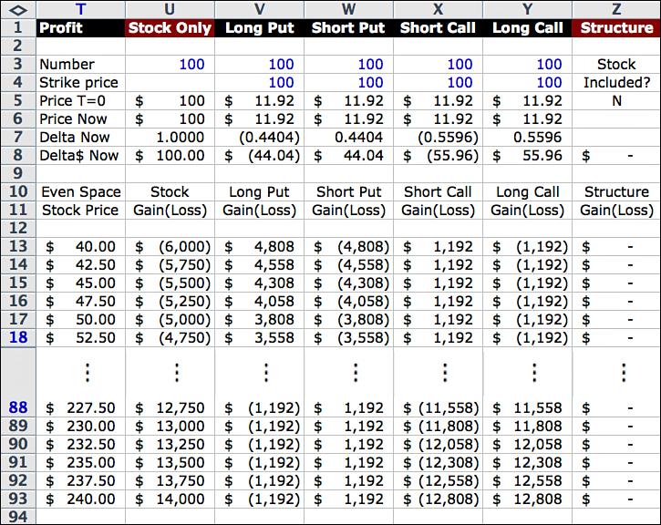
In this example, the number of shares of stock is 100. Strike prices are $100, and the prices of the options are all equal to $11.92. The Excel formulas for option profits corresponding to the previous definitions for Row 13 are:

V13 = V$3 × (MAX(0,V$4 – $T13) – V$5)

W13 = W$3 × (–MAX(0,W$4 – $T13) + W$5)

X13 = X$3 × (–MAX(0,$T13– X$4) + X$5)

Y13 = Y$3 × (MAX(0,$T13 – Y$4) – Y$5)

Z13 = SUM(U13:Y13)

To complete the section, copy these formulas down through Row 93.

The Black-Scholes formula price of this put option is $11.92. For now, hardcode this number in Cells V5 and V6. Later, in the section on the Black-Scholes formula, we will add the calculation and replace the hardcoded number with a new cell reference.

A long put option gives you the right to sell the underlying security for the strike price. It pays the difference between the strike price and the stock price at expiration, if the stock price is below the strike price. It pays nothing if the stock price is above the strike price. In Row 13, for instance, the stock price is $60 below the strike price, so the long put option pays $60 per share, or $6,000 in total based on 100 shares.

The payoff is $6,000, but the profit must be adjusted for the cost of the put option. In general, the profit on the transaction is the payoff minus the amount paid for the option. The profit is $4,808 ($6,000 − $1,192). That is the number in Cell V13. Similarly, when the stock price is $45, the profit is $4,308, and so on.

The short put profit is adjusted for the proceeds you received from selling the option. For example, in Row 13 the $6,000 loss is adjusted for the proceeds from selling the put option of $1,192. The net effect is a loss of $4,808 shown in Cell W13.

The calculations for short and long calls are similar.

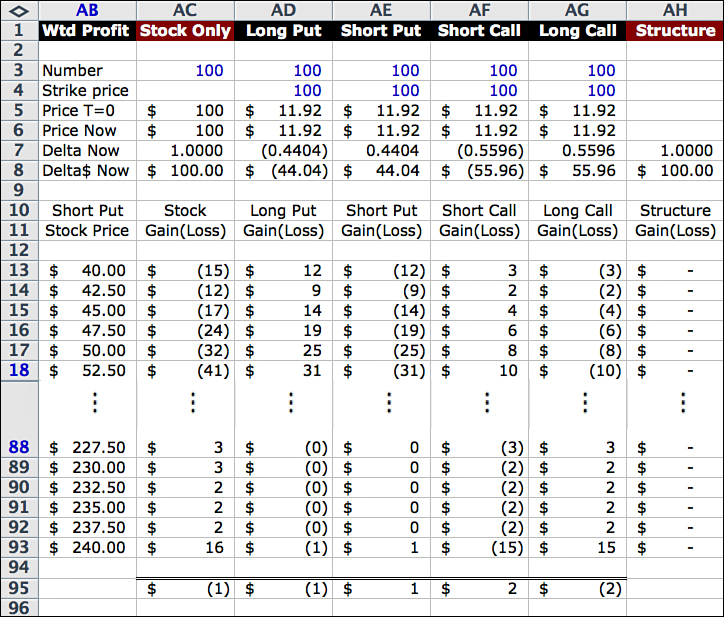
The answer is zero, or very close, for both stock and options. The answers are slightly off because the model is not exact. This is a reminder that the model assumes a world in which only 81 possible stock prices exist, so there are 81 possible payoffs for the stock and the options positions. Even so, the answers are close.

The stock outcome of zero makes sense because there is no assumed drift in the stock price under these assumptions. If the drift were 5%, expected profit on the stock would also be 5%. The options outcome of zero also makes sense. This is because we are valuing the options under the same assumptions used to price them. If there were a built-in gain or loss from simply buying or selling an option, it would be an arbitrage opportunity. If the option is priced correctly, adding the option to your portfolio does nothing to change the value of the portfolio at the moment you buy it. Of course, many people don’t think options are correctly priced, and they buy or sell them to take advantage of the mispricing. But that implies that the “real” probabilities or some other aspect of the assumptions are different from those assumed in pricing. That may be a great reason to trade, but for the model, it is a good sign that the expected values are zero.

To see why the answers are zero, let’s change the formulas in the Profit Diagram to exclude the option premiums. In other words, let’s set the values to the payoffs instead of profits. Actually, that puts the calculation back to option pricing, where the price of an option is the expected value of the option payoff random variable.

Figure 9.3 summarizes this.

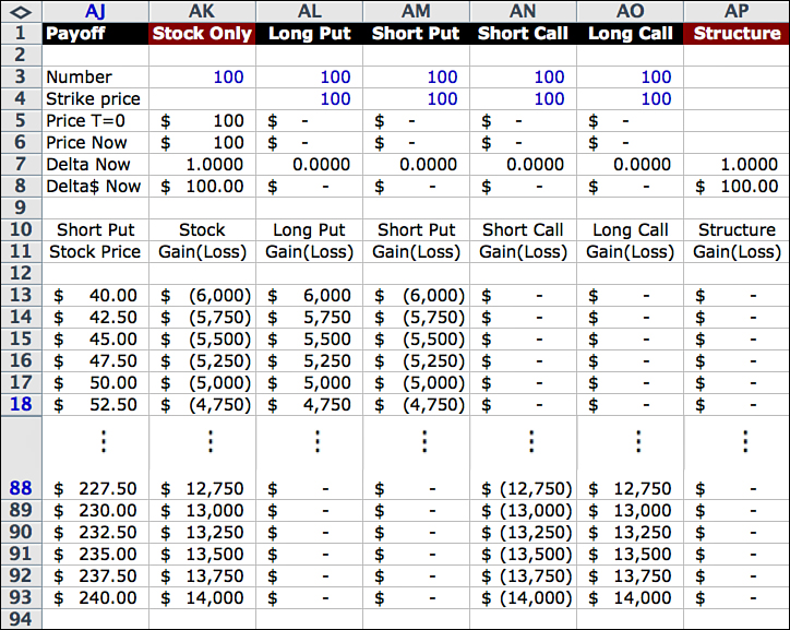
For this figure, the Profit Calculator columns were copied and pasted into Columns AJ through AP. Then the option prices in Rows 5 and 6 were set to zero. By doing this, the module calculates the payoff rather than the net payoff (or profit). This is similar to the procedure for option pricing, which means it should produce the same result, and it does.

Figure 9.4 is the same as Figure 9.3, except that the payoffs are multiplied by the probabilities.

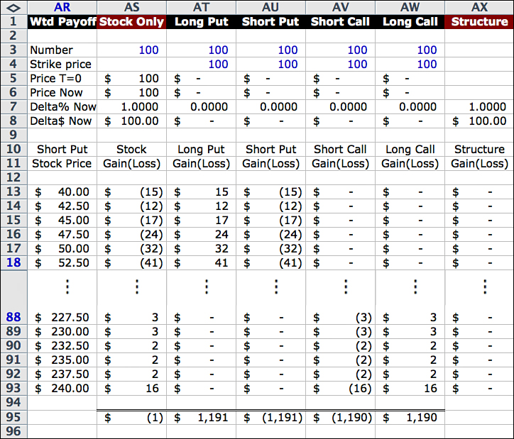
This illustrates, once more, that option prices are the weighted payoffs or the expected values of the payoff random variables. The only difference is that the answers refer to the total value of the options, given the number of options specified in the heading. Earlier, the option price was for one option. Here the value of the options represents 100 options. If you set Row 3 equal to 1 instead of 100, it would give you the price for one option.

With the number of options set to one, the price is $11.91 for the put options and $11.90 for the call options, compared to the Black-Scholes formula answers of $11.92.

The mathematical notation for expected value of the random variable X is E[X]. Using this notation, the relationship between the profit and payoff random variables is:

E[Stock Profit at Time 0] = Assumed stock price drift

E[Option Profit at Time 0] = $0

E[Option Payoff at Time 0] = The value of the options

And when the number of options is 1

E[Option Payoff at Time 0] = The option price

The last three exhibits were included only to illustrate the relationships between payoffs, profits, and expected values. They are not part of the model, but they do bring up a good question: What is the best—or easiest—way to price options in the model?

The advantage of using the Black-Scholes calculator is that you can copy it directly under the profit columns. It doesn’t require additional columns, and later when we look at multiple occurrences of option types, you don’t have to think about making changes to other parts of the spreadsheet. Because it is compact, it is easy to copy it twice to provide prices both at Time 0 and at the current date. Doing this with expected payoff columns would be more complicated.

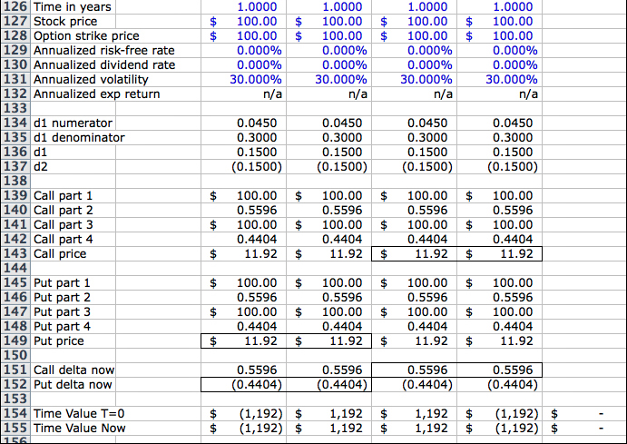
Figure 9.5 shows the Black-Scholes formula add-in. This is a view of Rows 97–152 in Columns T–Z, just below the Profit Calculator. The descriptions in the first column and the formulas in the second column are exactly the same as those in Chapter 3, with the exception of the deltas in Rows 151 and 152, which are explained later.

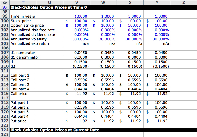
To create this section, copy the three-column Black-Scholes calculator from Chapter 3 into Columns T–V and define the input cells as:

V99 = $B$3 / 365

V100 = $B$4

V101 = V$4

V102 = $B$5

V103 = $B$6

V104 = $B$7

Next, copy the formulas in Column V across through Column Y. That completes the Time 0 section. Then copy and paste to create the current date section, changing B to C in the cell references to match the display screen inputs for time Current Date. The input cells on the display screen under Time 0 (Column B) will feed the Time 0 section, and the input cells on the display screen under current date (Column C) will feed the current date section.

Then set the stock prices in U5 = B4 and U6 = C4. These are also input items that you select. Next, set the option prices in Rows 5 and 6 equal to the values from the Black-Scholes add-in. These numbers are calculated based on the assumptions and scenarios you choose. The references are:

V5 = V122

W5 = W122

X5 = X116

Y5 = Y116

V6 = V149

W6 = W149

X6 = X143

Y6 = Y143

To finish, set the Deltas in Row 7 to the values from the Black-Scholes add-in, and define the $Deltas in Row 8 as:

V7 = V152

W7 = W152

X7 = X151

Y7 = Y151

V8 = V3 * V7

W8 = W3 * W7

X8 = X3 * X7

Y8 = Y3 * Y7

V151 = EXP(–V130 * V126) * V140

V152 = EXP(–V130 * V126) * V148

Copy these formulas across through Row Y to complete the section.

V154 = –V3 * (V5 – (MAX(0,V4 – $B$4)))

W154 = W3 * (W5 – (MAX(0,W4 – $B$4)))

X154 = X3 * (X5 – (MAX(0,$B$4 – X4)))

Y154 = –Y3 * (Y5 – (MAX(0,$B$4 – Y4)))

Z154 = SUM(V154:Y154)

V155 = –V3 * (V6 – (MAX(0,V4 – $C$4)))

W155 = W3 * (W6 – (MAX(0,W4 – $C$4)))

X155 = X3 * (X6 – (MAX(0,$C$4 – X4)))

Y155 = –Y3 * (Y6 – (MAX(0,$C$4 – Y4)))

Z155 = SUM(V155:Y155)

The numbers in Z154 and Z155 are shown on the display page as Option Time Value in Cells B9 and C9, respectively. To keep track of gains and losses, we also need the total premium paid or received for the options. This is the number of options multiplied by the premium for one option, with a negative sign for long positions, as follows:

V157 = –V3 * V5

W157 = W3 * W5

X157 = X3 * X5

Y157 = –Y3 * Y5

V158 = –V3 * V6

W158 = W3 * W6

X158 = X3 * X6

Y158 = –Y3 * Y6

The premiums in Row 157 are shown on the display page as Cash at Time 0, and the premiums in Row 158 are shown as Cash Now. Positive amounts indicate cash was paid for the option (long positions), and negative amounts mean cash was received for the option (short positions).