13. The Greeks

The Greeks measure the sensitivity of derivative prices to changes in pricing variables such as time, the price of the underlying security, interest rates, and volatility. The name comes from the Greek letters used to represent them. Normally, the Greeks refer to options, although they can apply to any derivative. The concept also extends to any structured security that contains derivatives.

Delta and theta, discussed throughout the book, are two of the option Greeks. In this chapter, these and other Greeks are presented more formally. Also, beginning with this material, we shift focus from attributing changes in value to understanding how to manage those changes.

To illustrate the difference in contexts, think about the term investment vehicle as a car metaphor. The earlier chapters on the elements of structured securities can be viewed as designing the car’s performance and safety features (engine power, the suspension, and braking distance, for example). Then in Chapter 12, “Understanding Price Changes,” we looked at the factors influencing option values, primarily over the longer term. The discussion on the changes in value due to pricing assumptions was similar to planning a trip, estimating how long it would take and what might happen along the way.

Now we focus on the shorter term. In the next three chapters, we look at how to drive the car. This is where the Greeks are useful. To take advantage of the increased flexibility of structured securities, it is important to have a good dashboard that tells you how fast you are going, how much gas is in the tank, and has a “check engine” light. The Greeks are part of that dashboard, providing real-time information to make tactical adjustments in risk–return profiles. The shorter-term nature of the Greeks make them valuable tools for measuring and managing portfolio positions.

When Greeks measure changes with respect to one of the pricing variables directly, they are known as first-order Greeks. There are also second-order Greeks, which measure changes with respect to another Greek. Gamma is an example of a second-order Greek. Gamma is the change in delta that results from a $1 increase in the stock price. The following are the most common Greeks:

• Delta: First order, related to stock price

• Theta: First order, related to time until expiration

• Rho: First order, related to risk-free rate

• Vega: First order, related to volatility

• Gamma: Second order, related to delta

Because option values change whenever one of the pricing variables changes, and the pricing variables can all be changing at once, how do you measure the effects of just one variable?

The assumption is this: When measuring the effect of one variable on option price, it is assumed that the other variables are constant. In reality, it is difficult to strictly isolate one of the pricing variables from the others. Pricing variables are in constant change. Time is always moving. Stock prices move during trading hours and after hours. Volatility is, well, volatile. But to make these calculations, some assumption has to be made about what is going on with the other variables. As you consider the Greeks, keep in mind the assumption behind them:

Each Greek measures the change in option price with respect to a small change in one variable, assuming the other variables are constant.

That is why the Greeks are somewhat theoretical. Still, over small time intervals, they provide practical information for managing options positions. They are indispensable to market makers and other market participants who need to adjust risk exposures rapidly. By measuring the component risks separately, these investors can rebalance a portfolio of options positions to achieve a desired exposure. For example, delta hedging refers to the practice of adjusting the number of shares of stock held in the portfolio in order to offset the change in value of the options positions.

As a reminder of a point made earlier in the book, when I use the term stock, I am really referring to any underlying security (including ETFs) that provide exposures to any number of assets and asset classes, including individual stocks, equity indexes, fixed income, interest rates, real estate, currencies, commodities, and other assets. So rather than being precise by using the term “underlying security,” I use stock to indicate the most common underlying security. However, I don’t want to give the impression that structured securities, or the Greeks, are restricted to equities.

Although I use the term more loosely to describe changes in an option with respect to changes in stock price, the Greeks technically describe changes in any derivative with respect to its underlying security. The same principles apply, for example, to a fixed-income portfolio or a commodity portfolio.

The second way to calculate option Greeks is to use a model or simulation tool. Because Black-Scholes prices European options under a fairly restrictive assumption set (including constant volatility over the option term), more accurate models, such as the binomial model, are often used to calculate Greeks. But with these models, there might not be a closed-form solution. In this case, you can obtain the Greeks by changing pricing variables and observing the change in the option price.

As a practical matter, most portfolio management is done with trading platforms. The platforms calculate the Greeks for you, although depending on the platform, it might use the Black-Scholes formula as an approximation to more exact American option pricing. Option trading platforms are provided by most asset-management firms and from specialty brokers such as TradeStation, optionMONSTER, thinkorswim, Interactive Brokers, and optionsXpress. The platforms are powerful and constantly improving. One recently introduced a probability distribution similar to the one developed in this book. Chapters 14, “Managing Positions,” and 15, “More on Synthetic Annuities,” introduce the TradeStation platform and use it to illustrate a synthetic annuity.

Y = X²

The derivative of Y with respect to X, denoted as dY/dX, measures the instantaneous rate of change in Y, given a specific value of X. For many formulas, the derivative can be solved and expressed as another formula. In this case, the derivative is:

dY/dX = 2X

If X = 0, the rate of change in Y at that specific point is 2X = 0. If X = 1, the rate of change in Y is 2. This illustrates a property of derivatives. The rate of change depends on the specific value of X.

The Greeks are a little more complicated. That is because the value of an option depends on six pricing variables. Of the six variables, only four can change after a specific option is chosen. For example, if you buy an option with a strike price of $100 and the underlying stock does not pay a dividend, those two pricing variables are fixed and will not change during the option term (the company could announce a dividend, but let’s assume that doesn’t happen). That leaves four pricing variables that can change.

The value of the option can and will change as (1) time (t) passes, (2) with changes in stock price (S), (3) as interest rates (r) change and (4) as volatility (σ) changes. If the value of the option is V, then:

V = f(t, S, r, σ)

When a function such as V depends on more than one variable, and you want to calculate a derivative, you have to be specific about what derivative means. For instance, if you want to know how V changes with respect to S, you need to specify exactly what is going on with t, r, and σ.

To make the solution manageable, the assumption is that the variables are constant. To make it clear that a derivative is being calculated under this assumption, the term partial derivative is used. It reminds you that the derivative is being calculated with respect to one variable—assuming that the other variables are constant. Delta, for instance, measures the rate of change of the option value V with respect to changes in the stock price S, with all other pricing variables constant. This assumption leads to restrictions on the interpretation of the derivative, but within narrow ranges (of time, stock price, and volatility), is a useful approximation.

Under the Black-Scholes pricing assumptions, it is possible to derive formulas for the Greeks.

The solution for a call option is:

e^–qτΦ(d₁)

where q is the dividend yield, t is the time to maturity, and

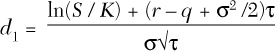
This formula for delta is used in the model and contained in the Black-Scholes add-in at the bottom of the Profit Calculator. Call and put deltas are calculated in Rows 151 and 152, respectively (refer to Figure 9.5 in Chapter 9) and are also displayed in Row 10, Columns E–J of the display screen.

If you look at the formulas for delta in the model, you will see that the formulas are not as complex as the previous expression. The reason is that the term d₁ was saved as an intermediate step in the Black-Scholes calculation. See, for example, Row 136 under the column for a short or long call. With d₁ available, delta is simplified to the first line of the delta expression above.

Delta, in this case, is 0.5596, or 55.96%, in Row 136 of the Profit Calculator. By definition, this is the delta of one share. This means that the option value is changing at the rate of 0.5596 when the stock price changes by $1. But remember, we have to be specific about the value of S and about the values of the other pricing variables. Here is almost the exact language:

The option value is changing at the rate of 0.5596 as the stock price changes from $100 to $101, with the other pricing variables being held constant at t = 1 year, r = 0%, and σ = 30%.

I say almost because the instantaneous rate of change applies to only an infinitely small range around $100, not to the entire range between $100 and $101. Technically, the rate of change increases at a different rate as the stock price moves to $101.01. By the time the stock price reaches $101, delta is changing at a new, higher rate. But the approximation is close enough for most purposes.

On the model display page, delta is scaled for the size of the option position. In Figure 13.1, delta shown in Cell I10 is equal to $55.96, or 100 times the per-share value.

In practical terms, how should you interpret this? The model compares two alternatives: a stock-only investment and a specified structured security. Here the structured security is one long call option contract covering 100 shares. If you buy 100 shares of stock and the stock price increases by $1, the position value increases in value by $100 (Cell E10). On the other hand, if you buy an option contract and the stock price increases by $1, delta tells you that the option position should increase in value by about $55.96.

You can see how much the value of the option actually increases by changing the stock price in the model from $100 to $101, as in Figure 13.2.

The option price changes from $11.92 to $12.49. This creates a position gain of $56.62, as shown in Cells I9 and J9. This is close to the delta estimate of $55.96. The difference results from the fact that delta increases as the stock price increases. At a stock price of $101, delta is $57.27, as shown in Cells I10 and J10. It makes sense that the actual change in option price is somewhere between the delta rate of $55.96 that applies at a stock price of $100 and the delta rate of $57.27 that applies at a stock price of $101. The only time $55.96 is an exact number is when the stock price is exactly $100.

To avoid confusion, keep in mind that delta can be expressed in different ways. For the model, the deltas in Row 10 are expressed as dollar amounts and reflect the size of the stock or option position. In this case the position is 100 shares, so delta is $55.96, or 100 times the per-share delta of $0.5596. If the position were 200 shares, delta would be $111.92. For 200 shares, the display page would show a stock-only delta of $200 and a call option delta of $111.92, meaning the following:

The option position (two contracts, or 200 shares) increases in value by $111.92 when the stock position (200 shares) increases in value by $1 per share, or $200 for the total position.

This is also a 55.96% change ($111.92 ÷ $200.00 = 0.5596). For one option, or one option position, it is just as easy to use either the percentage or the dollar amount. When there is a complicated position involving several options positions and an underlying security, it is better to know how the structure as a whole is moving instead of tracking each individual piece.

Here is summary of delta expressions:

• For one share, delta can be expressed as a number (0.5596), a percentage (55.96%), or a dollar amount ($0.5596).

• For a position consisting of more than one share, delta is normally expressed as a dollar amount. For a 100-share position, delta is shown as $55.96. You can also express delta as a percentage by dividing the dollar delta of the structure by the dollar delta of the stock, or 55.96% = $55.96 ÷ $100.

• In the model, delta in Row 10 will always be expressed as a dollar amount scaled to the position size.

One of the reasons for building the model was to allow you to look at any combination of stocks and options. Using the model, you can increase the stock price by $1 and see what happens to the value of the options and the structure as a whole. If you are looking at a single option position, you can use a platform or websites such as www.hoadley.net to produce tables and graphs illustrating how the Greeks behave under different conditions. When the position is more complicated, you can use the model to generate these tables and graphs. As illustrated in the next section, you can run whatever scenario you like, including multiple steps to create a delta table.

The bold highlighted row is the current situation: 22 days until expiration, a stock price of $105, and implied volatility of 37%. The value of the stock-only position is $31,500, and the value of the SynA is $30,381. The current delta of the stock-only position is $300 (by definition), and the current delta of SynA is $119.

The question is, how does the delta of this particular SynA behave in the short term with a sudden change in stock price? To answer this question, the days until expiration and volatility are held constant, and the stock and SynA values are determined by increasing and decreasing the stock price. For example, in Row 6, the stock price is assumed to jump to $110. At $110, the stock-only value goes from $31,500 to $33,000 (a $5 increase in price times 300 shares). At the same time, the SynA value goes up only about $500 ($30,882 − $31,500).

Notice also the pattern of increases. Column F shows how much the SynA value changes with each $1 increase in the stock price. Between $105 and $106, the SynA value increases by $115. But between $109 and $110, it goes up by only $85. This is an important property of delta for positions with short calls.

As the stock price increases, the value of the position goes up by smaller amounts.

The opposite is true when the stock price goes down. As the stock price falls from $105 to $104, the value of the SynA decreases by $123. But from $101 to $100, the value goes down by $145. There is a significant damping effect compared to the stock-only position (which goes down by $300, regardless of stock price level), but the damping effect is smaller with further price drops. The general rule for delta, whether for calls or puts, is:

The more in-the-money an option is, the higher the delta. And the more out-of-the-money an option is, the lower the delta.

The pattern of delta changes depends on the specific components of the structured security. One of the important aspects of planning for and monitoring delta is to understand the pattern of change. An easy way to do that is to create the delta table. To create a table, run the model once for each row. You can step through it manually, or you can set up a macro to run through the stock prices.

In terms of formulas, Cell F11 ($119) is delta from the model. The other values of Column F are the differences in consecutive values of Column E. For example, F10 = E10 − E11. Column G is Column F divided by the stock-only delta of $300. The SynA delta goes from 28% to 48% of the stock-only delta, even within this fairly narrow range of stock prices.

Theta can be calculated with the following formula:

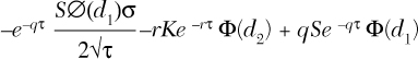
In this expression, the Greek symbol in the numerator of the first term represents the normal density function, and the Greek symbol in the second and third terms represents the normal cumulative density function.

Theta is like delta, in the sense that it is nonexact and constantly changing. And this expression applies only to a single option. Instead of going through the calculation in detail, it might be more instructive to walk though an example using the model and then discuss some practical issues.

There is a slight disconnect between the formal partial derivative definition given earlier and the more commonly used definition of theta as the change in value over one day. It is the same issue raised for delta, the distinction between the “instantaneous” nature of the partial derivative and the “over a period of one day” practical definition. The model conforms better to the one-day definition because it measures exactly that.

In this case, the value of the SynA increases by $14.99 over a one-day period. For reference, the instantaneous value of theta is close to $14 because it technically measures the change in value of a single instant of time at 24 hours remaining. Both the magnitude and pattern of change are important. Notice how theta changes over the 22 days until expiration.

On the first day, it is $14.99. Close to expiration, it is over $40.

The wide variation in theta over relatively small periods is the reason the model includes a modified version of theta, or average annualized theta. Average annualized theta is shown on the display page in Cells B10 and C10. This measure averages the effects of shorter-term thetas over the remaining option term.

For example, the value of the SynA in Figure 13.4 at expiration is $30,991, compared to $30,381, with 22 days left in the option term. The difference, $610, is due solely to the effect of time because the other variables were held constant.

Average daily time decay = $610 ÷ 22 days = $27.7272

On an annualized basis, this is:

Annualized average time decay = $27.2772 × 365 = $10,120

Expressed as a percentage of the position value, this is:

Average annualized theta = $10,120 ÷ $30,381 = 33.3%

In the table, theta expressed in these terms varied from 18.0% on Day 22 to 50.8% on the next-to-last day. It makes sense that the average value falls close to the middle of this range.

Look at this again with regard to Figure 13.1. In the figure:

B9 = $1,192.35

C9 = $1,148.97

The formulas for these two cells are:

B9 = Z156

C9 = Z157

Z156 and Z157 are developed as:

V156 = –V$3 × (V$5 − (MAX(0,V$4 − $B$4)))

W156 = W$3 × (W$5 − (MAX(0,W$4 − $B$4)))

X156 = X$3 × (X$5 − (MAX(0,$B$4 − X$4)))

Y156 = –Y$3 × (Y$5 − (MAX(0,$B$4 − Y$4)))

Z156 = SUM(V156:Y156)

V157 = –V$3 × (V6 − (MAX(0,V$4 − $C$4)))

W157 = W$3 × (W6 − (MAX(0,W$4 − $C$4)))

X157 = X$3 × (X6 − (MAX(0,$C$4 − X$4)))

Y157 = –Y$3 × (Y6 − (MAX(0,$C$4 − Y$4)))

Z157 = SUM(V157:Y157)

These formulas are the time value portion of total option premium for each option type. The total time value is shown in Cells B9 and C9 of the display page, so you can track the amount of time value for any structured position.

Time value is converted into annualized average theta in the same way as earlier, as follows:

Average daily time decay = $1,192.35 ÷ 365 days = $3.2667

On an annualized basis, this is:

Annualized average time decay = $3.2667 × 365 = $1,192.35

Expressed as a percentage of the position value, this is:

Average annualized theta = $1,192.35 ÷ 10,000 = 11.92%

B9 = IF(B9 = 0,0, – (B9 × 365 / B3) / $E$7)

C9 = IF(C9 = 0,0, – (C9 × 365 / C3) / $E$7)

When the stock price increases to $101, the time value changes to $1,148.97 because part of the value is now intrinsic. As a consequence, the average annualized theta drops to 11.49% from 11.92%.

Stocks, bonds, and options all have two sources of yield. One is dependent on price direction; the other depends only on the passage of time. With equities, dividends represent the time-only source of yield, whereas capital gains depend on stock price direction. With fixed income, interest or coupon payments are the time-only source of yield, and bond price changes depend on the direction of interest rates. The same is true of options. There is both a directional component and a time-only component of yield. By overlaying short options on a stock or bond security, you create a hybrid vehicle, adding the option time component to the dividend or interest yields.

When designing structured securities, you can build in target levels of yield. These levels depend on how volatile the overall market is at the time and the combination of term and number of options.

Over longer periods, the effects of volatility are much more pronounced. It is not uncommon to see volatility spike over 40 during turbulent periods or to settle below 20 during calm periods.

Even in normal market conditions, changes in implied volatility for a single security create interesting trading opportunities. Several options brokerages and commentators follow these changes in implied volatility as indicators. Joe Cusick of optionsXpress, for example, includes a section called “Implied Volatility Mover” in his daily newsletter:

Commentary by Joe Cusick — December 10, 2012, http://marketing.optionsxpress.com/index.php/email/

Implied volatility in the options on Diamond Foods (DMND) is up, as shares fall Monday. ...Volume is a brisk 1.2 million shares and roughly 16,000 options traded. 11,000 puts and 5,000 calls so far and 30-day implied volatility in DMND options is up 20 percent to 69.

In terms of general risk management, it is important to stress test portfolios in anticipation of volatility changes. One of the most important aspects of management is to set risk tolerances that you are comfortable with and understand in advance what tools you have to manage that risk. The next two chapters look at some of the metrics and design considerations to think about in building positions and portfolios.