
23. Economic Analysis of Architectures
Arthur Dent: “I think we have different value systems.” Ford Prefect: “Well mine’s better.”
—Douglas Adams, Mostly Harmless
Thus far, we have been primarily investigating the relationships between architectural decisions and the quality attributes that the architecture’s stakeholders have deemed important: If I make this architectural decision, what effect will it have on the quality attributes? If I have to achieve that quality attribute requirement, what architectural decisions will do the trick?
As important as this effort is, this perspective is missing a crucial consideration: What are the economic implications of an architectural decision?
Usually an economic discussion is focused on costs, primarily the costs of building the system in the first place. Other costs, often but not always downplayed, include the long-term costs incurred through cycles of maintenance and upgrade. However, as we argue in this chapter, as important as costs are the benefits that an architectural decision may bring to an organization.
Given that the resources for building and maintaining a system are finite, there must be a rational process that helps us choose among architectural options, during both an initial design phase and subsequent upgrade periods. These options will have different costs, will consume differing amounts of resources, will implement different features (each of which brings some benefit to the organization), and will have some inherent risk or uncertainty. To capture these aspects, we need economic models of software that take into account costs, benefits, risks, and schedule implications.
23.1. Decision-Making Context
As we saw in Chapter 16, business goals play a key role in requirements for architectures. Because major architectural decisions have technical and economic implications, the business goals behind a software system should be used to directly guide those decisions. The most immediate economic implication of a business goal decision on an architecture is how it affects the cost of implementing the system. The quality attributes achieved by the architecture decisions have additional economic implications because of the benefits (which we call utility) that can be derived from those decisions; for example, making the system faster or more secure or easier to maintain and update. It is this interplay between the costs and the benefits of architectural decisions that guides (and torments) the architect. Figure 23.1 show this interplay.
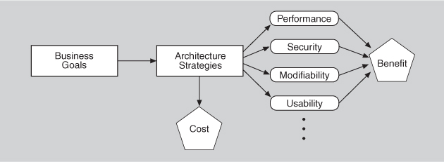
Figure 23.1. Business goals, architectural decisions, costs, and benefits
For example, using redundant hardware to achieve a desired level of availability has a cost; checkpointing to a disk file has a different cost. Furthermore, both of these architectural decisions will result in (presumably different) measurable levels of availability that will have some value to the organization developing the system. Perhaps the organization believes that its stakeholders will pay more for a highly available system (a telephone switch or medical monitoring software, for example) or that it will be sued if the system fails (for example, the software that controls antilock brakes in an automobile).
Knowing the costs and benefits associated with particular decisions enables reasoned selection from among competing alternatives. The economic analysis does not make decisions for the stakeholders, just as a financial advisor does not tell you how to invest your money. It simply aids in the elicitation and documentation of value for cost (VFC): a function of the costs, benefits, and uncertainty of a “portfolio” of architectural investments. It gives the stakeholders a framework within which they can apply a rational decision-making process that suits their needs and their risk aversion.
Economic analysis isn’t something to apply to every architectural decision, but rather to the most basic ones that put an overarching architectural strategy in place. It can help you assess the viability of that strategy. It can also be the key to objective selection among competing strategies, each of which might have advocates pushing their own self-interests.
23.2. The Basis for the Economic Analyses
We now describe the key ideas that form the basis for the economic analyses. The practical realization of these ideas can be packaged in a variety of ways, as we describe in Section 23.3. Our goal here is to develop the theory underpinning a measure of VFC for various architectural strategies in light of scenarios chosen by the stakeholders.
We begin by considering a collection of scenarios generated as a portion of requirements elicitation, an architectural evaluation, or specifically for the economic analysis. We examine how these scenarios differ in the values of their projected responses and we then assign utility to those values. The utility is based on the importance of each scenario being considered with respect to its anticipated response value.
Armed with our scenarios, we next consider the architectural strategies that lead to the various projected responses. Each strategy has a cost, and each impacts multiple quality attributes. That is, an architectural strategy could be implemented to achieve some projected response, but while achieving that response, it also affects some other quality attributes. The utility of these “side effects” must be taken into account when considering a strategy’s overall utility. It is this overall utility that we combine with the project cost of an architectural strategy to calculate a final VFC measure.
Utility-Response Curves
Our economic analysis uses quality attribute scenarios (from Chapter 4) as the way to concretely express and represent specific quality attributes. We vary the values of the responses, and ask what the utility is of each response. This leads to the concept of a utility-response curve.
Each scenario’s stimulus-response pair provides some utility (value) to the stakeholders, and the utility of different possible values for the response can be compared. This concept of utility has roots that go back to the eighteenth century, and it is a technique to make comparable very different concepts. To help us make major architectural decisions, we might wish to compare the value of high performance against the value of high modifiability against the value of high usability, and so forth. The concept of utility lets us do that.
Although sometimes it takes a little prodding to get them to do it, stakeholders can express their needs using concrete response measures, such as “99.999 percent available.” But that leaves open the question of how much they would value slightly less demanding quality attributes, such as “99.99 percent available.” Would that be almost as good? If so, then the lower cost of achieving that lower value might make that the preferred option, especially if achieving the higher value was going to play havoc with another quality attribute like performance. Capturing the utility of alternative responses of a scenario better enables the architect to make tradeoffs involving that quality attribute.
We can portray each relationship between a set of utility measures and a corresponding set of response measures as a graph—a utility-response curve. Some examples of utility-response curves are shown in Figure 23.2. In each, points labeled a, b, or c represent different response values. The utility-response curve thus shows utility as a function of the response value.
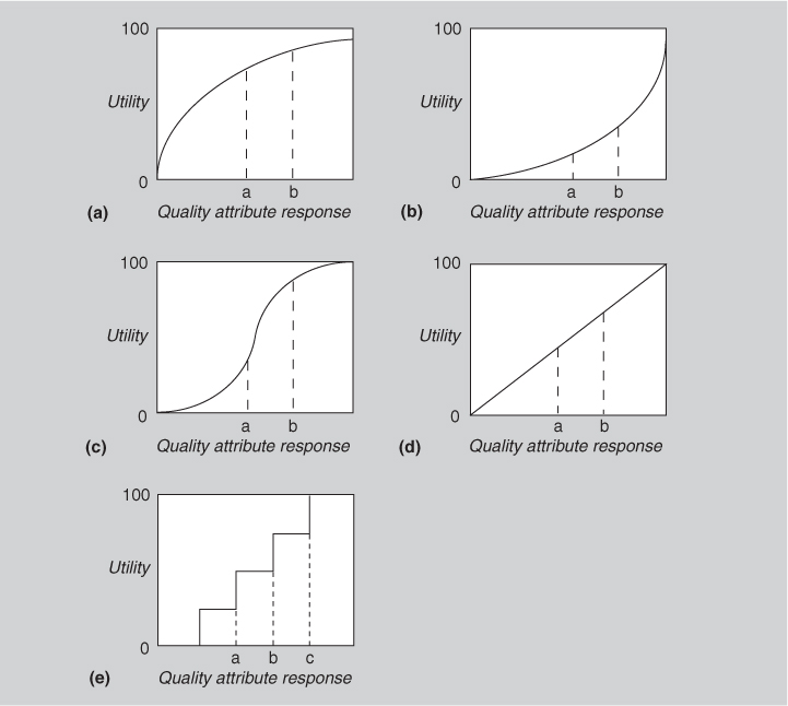
Figure 23.2. Some sample utility-response curves
The utility-response curve depicts how the utility derived from a particular response varies as the response varies. As seen in Figure 23.2, the utility could vary nonlinearly, linearly, or even as a step function. For example, graph (c) portrays a steep rise in utility over a narrow change in a quality attribute response level. In graph (a), a modest change in the response level results in only a very small change in utility to the user.
In Section 23.3 we illustrate some ways to engage stakeholders to get them to construct utility curves.
Weighting the Scenarios
Different scenarios will have different importance to the stakeholders; in order to make a choice of architectural strategies that is best suited to the stakeholders’ desires, we must weight the scenarios. It does no good to spend a great deal of effort optimizing a particular scenario in which the stakeholders actually have very little interest. Section 23.3 presents a technique for applying weights to scenarios.
Side Effects
Every architectural strategy affects not only the quality attributes it was selected to achieve, but also other quality attributes as well. As you know by now, these side effects on other quality attributes are often negative. If those effects are too negative, we must make sure there is a scenario for the side effect attribute and determine its utility-response curve so that we can add its utility to the decision-making mix. We calculate the benefit of applying an architectural strategy by summing its benefits to all relevant quality attributes; for some quality attributes the benefit of a strategy might be negative.
Determining Benefit and Normalization
The overall benefit of an architectural strategy across quality attribute scenarios is the sum of the utility associated with each one, weighted by the importance of the scenario. For each architectural strategy i, its benefit Bi over j scenarios (each with weight Wj) is
Bi = Σj (bi,j × Wj)
Referring to Figure 23.2, each bi,j is calculated as the change in utility (over whatever architectural strategy is currently in place, or is in competition with the one being considered) brought about by the architectural strategy with respect to this scenario:
bi,j = Uexpected – Ucurrent
That is, the utility of the expected value of the architectural strategy minus the utility of the current system relative to this scenario.
Calculating Value for Cost
The VFC for each architectural strategy is the ratio of the total benefit, Bi, to the cost, Ci, of implementing it:
VFC = Bi / Ci
The cost Ci is estimated using a model appropriate for the system and the environment being developed, such as a cost model that estimates implementation cost by measuring an architecture’s interaction complexity. You can use this VFC score to rank-order the architectural strategies under consideration.
Consider curves (a) and (b) in Figure 23.2. Curve (a) flattens out as the quality attribute response improves. In this case, it is likely that a point is reached past which VFC decreases as the quality attribute response improves; spending more money will not yield a significant increase in utility. On the other hand, curve (b) shows that a small improvement in quality attribute response can yield a very significant increase in utility. In that situation, an architectural strategy whose VFC is low might rank significantly higher with a modest improvement in its quality attribute response.
23.3. Putting Theory into Practice: The CBAM
With the concepts in place we can now describe techniques for putting them into practice, in the form of a method we call the Cost Benefit Analysis Method (CBAM). As we describe the method, remember that, like all of our stakeholder-based methods, it could take any of the forms for stakeholder interaction that we discussed in the introduction to Part III.
Practicalities of Utility Curve Determination
To build the utility-response curve, we first determine the quality attribute levels for the best-case and worst-case situations. The best-case quality attribute level is that above which the stakeholders foresee no further utility. For example, a system response to the user of 0.1 second is perceived as instantaneous, so improving it further so that it responds in 0.03 second has no additional utility. Similarly, the worst-case quality attribute level is a minimum threshold above which a system must perform; otherwise it is of no use to the stakeholders. These levels—best-case and worst-case—are assigned utility values of 100 and 0, respectively. We then determine the current and desired utility levels for the scenario. The respective utility values (between 0 and 100) for various alternative strategies are elicited from the stakeholders, using the best-case and worst-case values as reference points. For example, our current design provides utility about half as good as we would like, but an alternative strategy being considered would give us 90 percent of the maximum utility. Hence, the current utility level is set to 50 and the desired utility level is set to 90.
In this manner the utility curves are generated for all of the scenarios.
Practicalities of Weighting Determination
One method of weighting the scenarios is to prioritize them and use their priority ranking as the weight. So for N scenarios, the highest priority one is given a weight of 1, the next highest is given a weight of (N–1)/N, and so on. This turns the problem of weighting the scenarios into one of assigning priorities.
The stakeholders can determine the priorities through a variety of voting schemes. One simple method is to have each stakeholder prioritize the scenarios (from 1 to N) and the total priority of the scenario is the sum of the priorities it receives from all of the stakeholders. This voting can be public or secret.
Other schemes are possible. Regardless of the scheme used, it must make sense to the stakeholders and it must suit their culture. For example, in some corporate environments, everything is done by consensus. In others there is a strict hierarchy, and in still others decisions are made in a democratic fashion. In the end it is up to the stakeholders to make sure that the scenario weights agree with their intuition.
Practicalities of Cost Determination
One of the shortcomings of the field of software architecture is that there are very few cost models for various architectural strategies. There are many software cost models, but they are based on overall system characteristics such as size or function points. These are inadequate to answer the question of how much does it cost to, for example, use a publish-subscribe pattern in a particular portion of the architecture. There are cost models that are based on complexity of modules (by function point analysis according to the requirements assigned to each module) and the complexity of module interaction, but these are not widely used in practice. More widely used in practice are corporate cost models based on previous experience with the same or similar architectures, or the experience and intuition of senior architects.
Lacking cost models whose accuracy can be assured, architects often turn to estimation techniques. To proceed, remember that an absolute number for cost isn’t necessary to rank candidate architecture strategies. You can often say something like “Suppose strategy A costs $x. It looks like strategy B will cost $2x, and strategy C will cost $0.5x.” That’s enormously helpful. A second approach is to use very coarse estimates. Or if you lack confidence for that degree of certainty, you can say something like “Strategy A will cost a lot, strategy B shouldn’t cost very much, and strategy C is probably somewhere in the middle.”
CBAM
Now we describe the method we use for economic analysis: the Cost Benefit Analysis Method. CBAM has for the most part been applied when an organization was considering a major upgrade to an existing system and they wanted to understand the utility and value for cost of making the upgrade, or they wanted to choose between competing architectural strategies for the upgrade. CBAM is also applicable for new systems as well, especially for helping to choose among competing strategies. Its key concepts (quality attribute response curves, cost, and utility) do not depend on the setting.
Steps
A process flow diagram for the CBAM is given in Figure 23.3. The first four steps are annotated with the relative number of scenarios they consider. That number steadily decreases, ensuring that the method concentrates the stakeholders’ time on the scenarios believed to be of the greatest potential in terms of VFC.
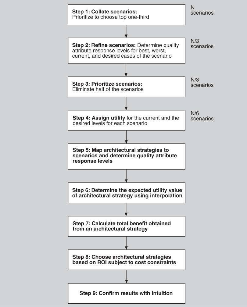
Figure 23.3. Process flow diagram for the CBAM
This description of CBAM assumes that a collection of quality attribute scenarios already exists. This collection might have come from a previous elicitation exercise such as an ATAM exercise (see Chapter 21) or quality attribute utility tree construction (see Chapter 16).
The stakeholders in a CBAM exercise include people who can authoritatively speak to the utility of various quality attribute responses, and probably include the same people who were the source of the quality attribute scenarios being used as input. The steps are as follows:
1. Collate scenarios. Give the stakeholders the chance to contribute new scenarios. Ask the stakeholders to prioritize the scenarios based on satisfying the business goals of the system. This can be an informal prioritization using a simple scheme such as “high, medium, low” to rank the scenarios. Choose the top one-third for further study.
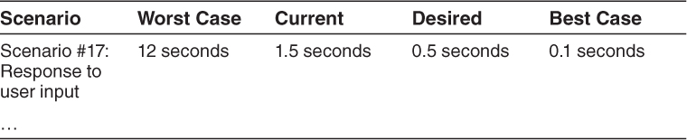
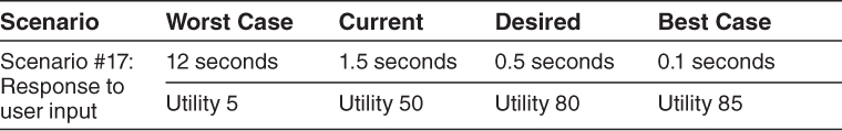
2. Refine scenarios. Refine the scenarios chosen in step 1, focusing on their stimulus-response measures. Elicit the worst-case, current, desired, and best-case quality attribute response level for each scenario. For example, a refined performance scenario might tell us that worst-case performance for our system’s response to user input is 12 seconds, the best case is 0.1 seconds, and our desired response is 0.5 seconds. Our current architecture provides a response of 1.5 seconds:
3. Prioritize scenarios. Prioritize the refined scenarios, based on stakeholder votes. You give 100 votes to each stakeholder and have them distribute the votes among the scenarios, where their voting is based on the desired response value for each scenario. Total the votes and choose the top 50 percent of the scenarios for further analysis. Assign a weight of 1.0 to the highest-rated scenario; assign the other scenarios a weight relative to the highest rated. This becomes the weighting used in the calculation of a strategy’s overall benefit. Make a list of the quality attributes that concern the stakeholders.
4. Assign utility. Determine the utility for each quality attribute response level (worst-case, current, desired, best-case) for the scenarios from step 3. You can conveniently capture these utility curves in a table (one row for each scenario, one column for each of the four quality attribute response levels). Continuing our example from step 2, this step would assign utility values from 1 to 100 for each of the latency values elicited for this scenario in step 2:
5. Map architectural strategies to scenarios and determine their expected quality attribute response levels. For each architectural strategy under consideration, determine the expected quality attribute response levels that will result for each scenario.
6. Determine the utility of the expected quality attribute response levels by interpolation. Using the elicited utility values (that form a utility curve), determine the utility of the expected quality attribute response level for the architectural strategy. Do this for each relevant quality attribute enumerated in step 3. For example, if we are considering a new architectural strategy that would result in a response time of 0.7 seconds, we would assign this a utility proportionately between 50 (which it exceeds) and 80 (which it doesn’t exceed).
The formula for interpolation between two data points (xa, ya) and (xb, yb) is given by:
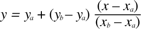
For us, the x values are the quality attribute response levels and the y values are the utility values. So, employing this formula, the utility value of a 0.7-second response time is 74.
7. Calculate the total benefit obtained from an architectural strategy. Subtract the utility value of the “current” level from the expected level and normalize it using the votes elicited in step 3. Sum the benefit due to a particular architectural strategy across all scenarios and across all relevant quality attributes.
8. Choose architectural strategies based on VFC subject to cost and schedule constraints. Determine the cost and schedule implications of each architectural strategy. Calculate the VFC value for each as a ratio of benefit to cost. Rank-order the architectural strategies according to the VFC value and choose the top ones until the budget or schedule is exhausted.
9. Confirm results with intuition. For the chosen architectural strategies, consider whether these seem to align with the organization’s business goals. If not, consider issues that may have been overlooked while doing this analysis. If there are significant issues, perform another iteration of these steps.
Computing Benefit for Architectural Variation Points
This chapter is about calculating the cost and benefit of competing architectural options. While there are plenty of metrics and methods to measure cost, usually as some function of complexity, benefit is more slippery. CBAM uses an assemblage of stakeholders to work out jointly what utility each architectural option will bring with it. At the end of the day, CBAM’s measures of utility are subjective, intuitive, and imprecise. That’s all right; stakeholders seldom are able to express benefit any better than that, and so CBAM takes what stakeholders know and formulates it into a justified choice. That is, CBAM elicits inputs that are imprecise, because nothing better is available, and does the best that can be done with them.
As a counterpoint to CBAM, there is one area of architecture in which the architectural options are of a specific variety: product-line architectures. In Chapter 25, you’ll be introduced to software architectures that serve for an entire family of systems. The architect introduces variation points into the architecture, which are places where it can be quickly tailored in preplanned ways so that it can serve each of a variety of different but related products. In the product-line context, the major architectural option is whether to build a particular variation point in the architecture. Doing so isn’t free; otherwise, every product-line architecture would have an infinitude of variation points. So the question becomes: When will adding a variation point pay off?
CBAM would work for this case as well; you could ask the product line’s stakeholders what the utility of a new variation point would be, vis-à-vis other options such as including a different variation point instead, or none at all. But in this case, there is a quantitative formula to measure the benefit. John McGregor of Clemson University has long been interested in the economics of software product lines, and along with others (including me) invented SIMPLE, a cost-modeling language for software product lines. SIMPLE is great at estimating the cost of product-line options, but not so great at estimating its benefits. Recently, McGregor took a big step toward remedying that.
Here is his formula for modeling the marginal value of building in an additional variation point to the architecture:
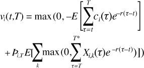
Got that? No? Right, me neither. But we can understand it if we build it up from pieces.
The equation says (as all value equations do) that value is benefit minus cost, and so those are the two terms.
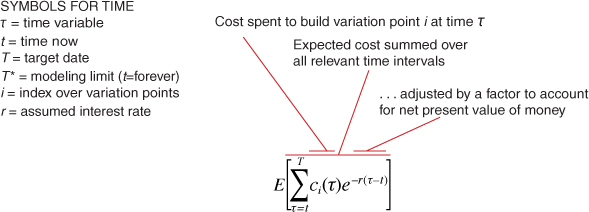
The first term measures the expected cost of building variation point i over a time period from now until time T (some far-off horizon of interest such as fielding your fifth system or getting your next round of venture capital funding). The function ci(τ) measures the cost of building variation point i at time τ; it’s evaluated using conventional cost-estimating techniques for software. The e factor is a standard economic term that accounts for the net present value of money; r is the assumed current interest rate. This is summed up over all time between now and T, and made negative to reflect that cost is negative value. So here’s the first term decomposed:
The second term evaluates the benefit. The function Xi,k(τ) is the key; it measures the value of the variation point in the kth product of the product line. This is equal to the marginal value of the variation point to the kth product, minus the cost of using (exercising) the variation point in that kth product. That first part is the hardest part to come by, but your marketing department should be able to help by expressing the marginal value in terms of the additional products that the variation point would enable you to build and how much revenue each would bring in. (That’s what marketing departments are paid to figure out.)
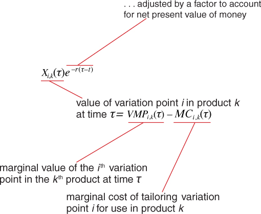
To the function X we apply the same factor as before to account for the net present value of money, sum it up over all time periods between now and T, and make it nonnegative:
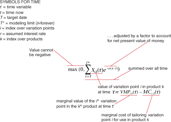
Then we sum that up over all products k in the product line and multiply it by the probability that the variation point will in fact be ready by the time it’s needed:
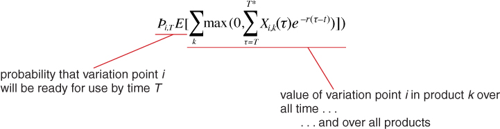
Add the two terms together and there you have it. It’s easy to put this in a spreadsheet that calculates the result given the relevant inputs, and it provides a quantitative measurement to help guide selection of architectural options—in this case, introduction of variation points to support a product line.
—PCC
23.4. Case Study: The NASA ECS Project
We will now apply the CBAM to a real-world system as an example of the method in action.
The Earth Observing System is a constellation of NASA satellites that gathers data for the U.S. Global Change Research Program and other scientific communities worldwide. The Earth Observing System Data Information System (EOSDIS) Core System (ECS) collects data from various satellite downlink stations for further processing. ECS’s mission is to process the data into higher-form information and make it available to scientists in searchable form. The goal is to provide both a common way to store (and hence process) data and a public mechanism to introduce new data formats and processing algorithms, thus making the information widely available.
The ECS processes an input stream of hundreds of gigabytes of raw environment-related data per day. The computation of 250 standard “products” results in thousands of gigabytes of information that is archived at eight data centers in the United States. The system has important performance and availability requirements. The long-term nature of the project also makes modifiability important.
The ECS project manager had a limited annual budget to maintain and enhance his current system. From a prior analysis—in this case an ATAM exercise—a large set of desirable changes to the system was elicited from the system stakeholders, resulting in a large set of architectural strategies. The problem was to choose a (much) smaller subset for implementation, as only 10 to 20 percent of what was being proposed could actually be funded. The manager used the CBAM to make a rational decision based on the economic criterion of return on investment.
In the execution of the CBAM described next, we concentrated on analyzing the Data Access Working Group (DAWG) portion of the ECS.
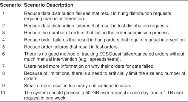
Step 1: Collate Scenarios
A subset of the raw scenarios put forward by the DAWG team were as shown in Table 23.1. Note that they are not yet well formed and that some of them do not have defined responses. These issues are resolved in step 2, when the number of scenarios is reduced.1
Table 23.1. Collected Scenarios in Priority Order
Step 2: Refine Scenarios
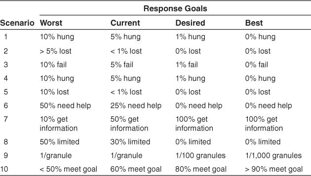
The scenarios were refined, paying particular attention to precisely specifying their stimulus-response measures. The worst-case, current-case, desired-case, and best-case response goals for each scenario were elicited and recorded, as shown in Table 23.2.
Table 23.2. Response Goals for Refined Scenarios
Step 3: Prioritize Scenarios
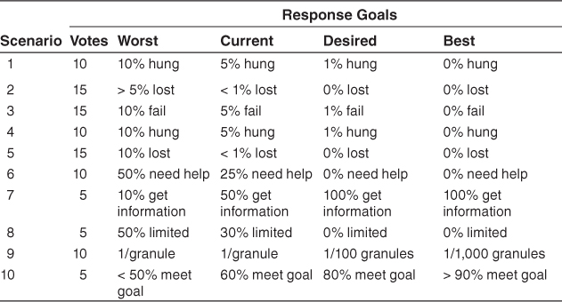
In voting on the refined representation of the scenarios, the close-knit team deviated slightly from the method. Rather than vote individually, they chose to discuss each scenario and arrived at a determination of its weight via consensus. The votes allocated to the entire set of scenarios were constrained to 100, as shown in Table 23.3. Although the stakeholders were not required to make the votes multiples of 5, they felt that this was a reasonable resolution and that more precision was neither needed nor justified.
Table 23.3. Refined Scenarios with Votes
Step 4: Assign Utility
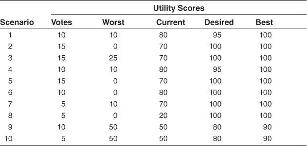
In this step the utility for each scenario was determined by the stakeholders, again by consensus. A utility score of 0 represented no utility; a score of 100 represented the most utility possible. The results of this process are given in Table 23.4.
Table 23.4. Scenarios with Votes and Utility Scores
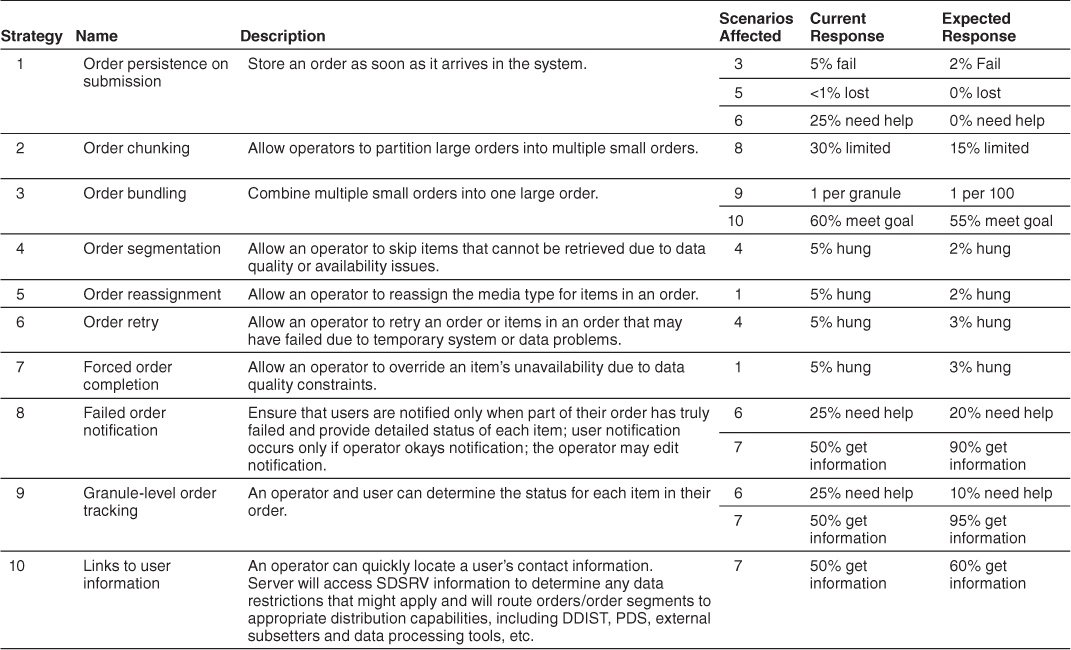
Step 5: Develop Architectural Strategies for Scenarios and Determine Their Expected Quality Attribute Response Levels
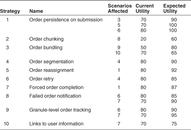
Based on the requirements implied by the preceding scenarios, a set of 10 architectural strategies was developed by the ECS architects. Recall that an architectural strategy may affect more than one scenario. To account for these complex relationships, the expected quality attribute response level that each strategy is predicted to achieve had to be determined with respect to each relevant scenario. The set of architectural strategies, along with the determination of the scenarios they address, is shown in Table 23.5. For each architectural strategy/scenario pair, the response levels expected to be achieved with respect to that scenario are shown (along with the current response, for comparison purposes).
Table 23.5. Architectural Strategies and Scenarios Addressed
Step 6: Determine the Utility of the “Expected” Quality Attribute Response Levels by Interpolation
Once the expected response level of every architectural strategy has been characterized with respect to a set of scenarios, their utility can be calculated by consulting the utility scores for each scenario’s current and desired responses for all of the affected attributes. Using these scores, we may calculate, via interpolation, the utility of the expected quality attribute response levels for the architectural strategy/scenario pair applied to the DAWG of ECS.
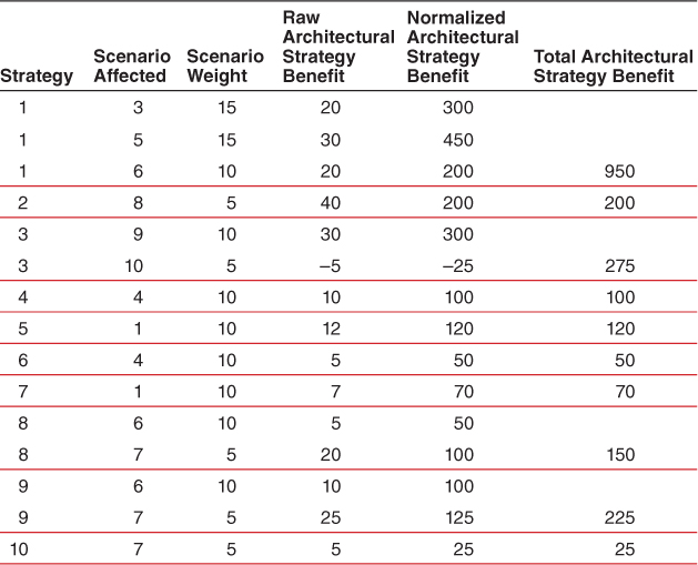
Step 7: Calculate the Total Benefit Obtained from an Architectural Strategy
Based on the information collected, as represented in Table 23.6, the total benefit of each architectural strategy can now be calculated, following the equation from Section 23.2, repeated here:
Bi = Σj (bi, j × Wj)
Table 23.6. Architectural Strategies and Their Expected Utility
This equation calculates total benefit as the sum of the benefit that accrues to each scenario, normalized by the scenario’s relative weight. Using this formula, the total benefit scores for each architectural strategy are now calculated, and the results are given in Table 23.7.
Table 23.7. Total Benefit of Architectural Strategies
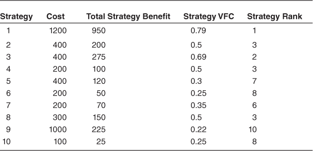
Step 8: Choose Architectural Strategies Based on VFC Subject to Cost Constraints
To complete the analysis, the team estimated cost for each architectural strategy. The estimates were based on experience with the system, and a return on investment for each architectural strategy was calculated. Using the VFC, we were able to rank each strategy. This is shown in Table 23.8. Not surprisingly, the ranks roughly follow the ordering in which the strategies were proposed: strategy 1 has the highest rank; strategy 3 the second highest. Strategy 9 has the lowest rank; strategy 8, the second lowest. This simply validates stakeholders’ intuition about which architectural strategies were going to be of the greatest benefit. For the ECS these were the ones proposed first.
Table 23.8. VFC of Architectural Strategies
Results of the CBAM Exercise
The most obvious results of the CBAM are shown in Table 23.8: an ordering of architectural strategies based on their predicted VFC. However, just as for the ATAM method, the benefits of the CBAM extend beyond the qualitative outcomes. There are social and cultural benefits as well.
Just as important as the ranking of architectural strategies in CBAM is the discussion that accompanies the information-collecting and decision-making processes. The CBAM process provides a great deal of structure to what is always largely unstructured discussions, where requirements and architectural strategies are freely mixed and where stimuli and response goals are not clearly articulated. The CBAM process forces the stakeholders to make their scenarios clear in advance, to assign utility levels of specific response goals, and to prioritize these scenarios based on the resulting determination of utility. Finally, this process results in clarification of both scenarios and requirements, which by itself is a significant benefit.
23.5. Summary
Architecture-based economic analysis is grounded on understanding the utility-response curve of various scenarios and casting them into a form that makes them comparable. Once they are in this common form—based on the common coin of utility—the VFC for each architecture improvement, with respect to each relevant scenario, can be calculated and compared.
Applying the theory in practice has a number of practical difficulties, but in spite of those difficulties, we believe that the application of economic techniques is inherently better than the ad hoc decision-making approaches that projects (even quite sophisticated ones) employ today. Our experience with the CBAM tells us that giving people the appropriate tools to frame and structure their discussions and decision making is an enormous benefit to the disciplined development of a complex software system.
23.6. For Further Reading
The origins of the CBAM can be found in two papers: [Moore 03] and Kazman [01].
A more general background in economic approaches to software engineering may be found in the now-classic book by Barry Boehm [Boehm 81].
And a more recent, and somewhat broader, perspective on the field can be found in [Biffl 10].
The product-line analysis we used in the sidebar on the value of variation points came from a paper in the 2011 International Software Product Line Conference by John McGregor and his colleagues [McGregor 11].
23.7. Discussion Questions
1. This chapter is about choosing an architectural strategy using rational, economic criteria. See how many other ways you can think of to make a choice like this. Hint: Your candidates need not be “rational.”
2. Have two or more different people generate the utility curve for a quality attribute scenario for an ATM. What are the difficulties in generating the curve? What are the differences between the two curves? How would you reconcile the differences?
3. Discuss the advantages and disadvantages of the method for generating scenario priorities used in the CBAM. Can you think of a different way to prioritize the scenarios? What are the pluses and minuses of your method?
4. Using the results of your design exercise for the ATM from Chapter 17 as a starting point, develop an architectural strategy for achieving a quality attribute scenario that your design does not cover.
5. Generate the utility curves for two different systems in the same domain. What are the differences? Do you believe that there are standard curves depending on the domain? Defend your answer.