
8
Reorder and summarize data
In this chapter
One of the most important uses of business information is to keep a record of when something happens. Whether you ship a package to a client or pay a supplier, tracking when you took those actions, and in what order, helps you analyze your performance. Sorting your information based on the values in one or more columns helps you discover useful trends, such as whether your sales are generally increasing or decreasing, whether you do more business on specific days of the week, or whether you sell products to lots of customers from certain regions of the world.
Excel includes capabilities you might expect to find only in a database program: the ability to organize your data into levels of detail you can show or hide and formulas that let you look up values in a list of data. Organizing data by detail level lets you focus on specific aspects of the data, and looking up values in a worksheet helps you find specific data. If a customer calls to ask about an order, you can use the order number or customer number to discover the information that customer needs.
This chapter guides you through procedures related to sorting your data by using one or more criteria, sorting data against custom lists, outlining data, and calculating subtotals.
Sort worksheet data
Although Excel makes it easy to enter your business data and to manage it after you’ve saved it in a worksheet, unsorted data will rarely answer every question you want to ask. For example, you might want to discover which of your services generates the most profits or which service costs the most for you to provide. You can discover that information by sorting your data.
When you sort data in a worksheet, you rearrange the rows that contain the data based on the contents of cells in a specific column or set of columns. The first step in sorting a range of data is to identify the column or columns that contain the values by which you want to sort. You can sort by as many of the columns as you want to.
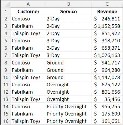
A data range sorted by Service and then Customer
If you want to sort data by only one column that contains words, numbers, or dates, you can quickly do so from the Home tab of the ribbon.
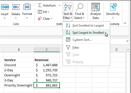
A simple sort from the ribbon
The options on the Sort & Filter menu vary depending on whether you’re sorting a column of words, numbers, or dates. Excel sorts words from A to Z or Z to A, numbers from smallest to largest or largest to smallest, and dates from newest to oldest or oldest to newest.
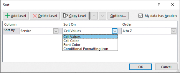
You perform multiple-column sort operations from the Sort dialog, in which you can specify the columns to sort by, the order in which to sort each column, and the order in which to perform the sort operations. When creating similar rules, you can save time by copying one rule and changing only the field name.
If cell values within the data range have font or fill colors applied to them, either manually or though conditional formatting, you can sort the data to place a specific color at the beginning or end of the column.
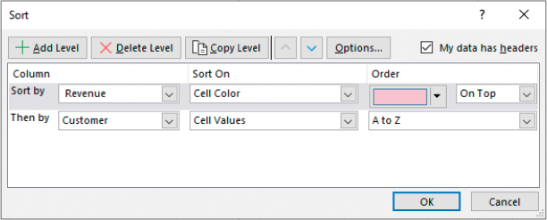
Sort by multiple columns and properties
You can easily change the order in which rules are applied, as well as edit and delete rules, in the Sort dialog.
To display the Sort & Filter menu
On the Home tab, in the Editing group, select Sort & Filter.
To sort a data range alphanumerically by a single column
Select a cell in the column by which you want to sort the data range.
Display the Sort & Filter menu.
Do either of the following:
Select Sort A to Z, Sort Smallest to Largest, or Sort Oldest to Newest to sort the data in ascending order.
Select Sort Z to A, Sort Largest to Smallest, or Sort Newest to Oldest to sort the data in descending order.
Or
Select the data range you want to sort or a cell in the range.
Display the Sort & Filter menu and then select Custom Sort.
If appropriate, select the My data has headers checkbox.
In the Sort by list, select the field by which you want to sort.
In the Sort On list, select Cell Values.
In the Order list, do either of the following:
Select A to Z or Smallest to Largest to sort the data in ascending order.
Select Z to A or Largest to Smallest to sort the data in descending order.
To sort a data range by cell color, font color, or icon
Select the data range you want to sort or a cell in the range.
Display the Sort & Filter menu, and then select Custom Sort.
If appropriate, select the My data has headers checkbox.
In the Sort by list, select the field by which you want to sort.
In the Sort On list, select Cell Color, Font Color, or Conditional Formatting Icon.
In the Order list, select the cell or font color or icon that you want to isolate. Then, in the last list box, do either of the following:
Select On Top to sort that color or icon to the beginning of the list.
Select On Bottom to sort that color or icon to the end of the list.
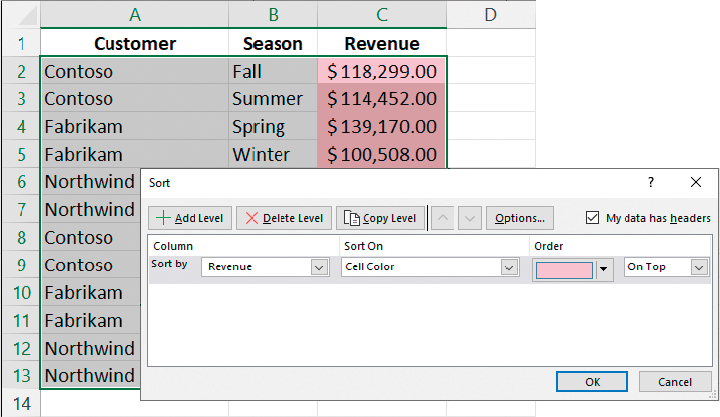
Sort lists of data using cell fill color as a criterion
Select OK to sort the values.
Or
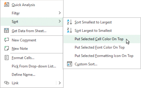
In the data range, right-click the cell that has the color or icon you want to isolate, and then on the context menu, select Sort.
 Tip
TipTo display a context menu, right-click or long-press (tap and hold) the element.
On the Sort submenu, select Put Selected Attribute On Top.
Sort by multiple columns and properties
To sort a data range based on values in multiple columns
Select the data range you want to sort or a cell in the range.
On the Home tab, in the Editing group, select Sort & Filter.
On the Sort & Filter menu, select Custom Sort.
If appropriate, select the My data has headers checkbox.
In the Sort by list, select the first field by which you want to sort.
In the Sort On list, select the option by which you want to sort the data (Cell Values, Cell Color, Font Color, or Conditional Formatting Icon).
Create sorting rules in the Sort dialog
In the Order list, select an order for the sort operation.
For each additional column by which you want to sort, do the following:
Select Add Level.
In the Then by list, select the column.
Select values in the Sort On and Order lists.
Select OK to sort the values.
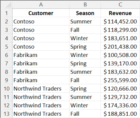
A data range sorted by Customer and then by Revenue
To copy a sorting level
In the Sort dialog, select the sorting level you want to copy.
Select the Copy Level button.
To move a sorting rule up or down in priority
In the Sort dialog, select the sorting rule you want to move.
Do either of the following:
Select the Move Up (^) button to move the rule earlier in the order.
Select the Move Down (v) button to move the rule later in the order.
To delete a sorting rule
In the Sort dialog, select the sorting level you want to delete.
Select Delete Level.
Sort data by using custom lists
By default, Excel sorts words in alphabetical order and numbers in numeric order. But that pattern doesn’t work for some sets of values. For example, if you’re sorting a series of months, alphabetical order begins with April and ends with September.
Fortunately, Excel recognizes days of the week and months of the year as special lists that it uses for sorting and when filling series. You can add custom series to Excel for the same purposes, either by entering the list values or copying them from a worksheet.
To define a custom list by entering its values
Display the Advanced page of the Excel Options dialog.
Scroll to the General section, and then select Edit Custom Lists.
In the Custom Lists dialog, with NEW LIST active, activate the List entries box.
Enter the custom list items in order, pressing Enter between items.
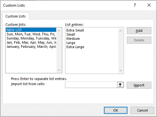
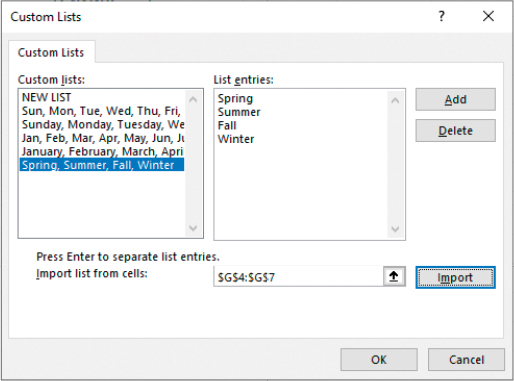
Manage lists in the Custom Lists dialog
After you enter all the list items, select Add to move them to the Custom Lists pane.
Select OK, and then select OK again to close the Excel Options dialog.
To define a custom list by copying values from a worksheet
Enter the custom list values in a column, in the correct sort order (first to last, from top to bottom), and then select the cells that contain the list values.
Open the Custom Lists dialog.
Verify that the Import list from cells box contains the correct cells, and then select Import.
Sort and fill series from any list
Select OK, and then select OK again to close the Excel Options dialog.
To sort worksheet data by using a custom list
Select a cell in the list of data you want to sort.
On the Home tab, select the Sort & Filter button, and then select Custom Sort.
If necessary, select the My data has headers checkbox.
In the Sort by list, select the field that contains the data by which you want to sort.
If necessary, in the Sort On list, select Values.
In the Order list, select Custom List.
In the Custom Lists dialog, select the list you want to use. Then select OK.
In the Sort dialog, select OK to close the dialog and sort the data.
Outline and subtotal data
When your data range is sorted into the order you want, you can use the Subtotal feature to have Excel outline the data by specific categories and summarize the categories. The available summary functions are SUM, COUNT, AVERAGE, MAX, MIN, PRODUCT, COUNT NUMBERS, STDDEV, STDDEVP, VAR, and VARP.
![]() Important
Important
You can outline, group, and summarize data ranges by using the SUBTOTAL feature; it does not work on data in Excel tables. To subtotal table data, you must first convert it to a range.
In a subtotal operation, you choose the column by which to group the data, the summary calculation you want to perform, and the values to be summarized. After you define the subtotals, Excel displays them in your worksheet.
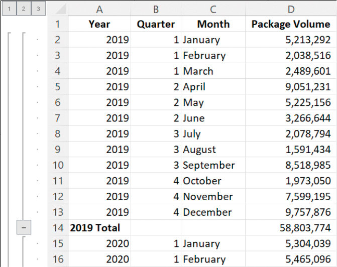
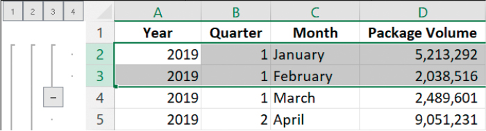
A data range with subtotal outlining applied
Excel also defines groups based on the subtotal calculation. The groups form an outline of the data based on the criteria you used to create the subtotals. For example, all the rows representing months in the year 2019 could be in one group, rows representing months in 2020 in another, and so on. You can use the controls in the outline area on the left side of the worksheet to hide or display groups of data.
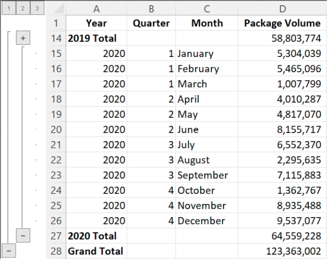
The data range with details for the year 2019 hidden
The numbers above the outline controls are the level buttons. Each represents a level of data organization. Selecting a level button hides all levels of detail below that of the button you selected.
The following table describes the data contained at each level of a worksheet with three levels of organization.
Level | Description |
|---|---|
1 | Grand total |
2 | Subtotals for each group |
3 | Individual rows in the worksheet |
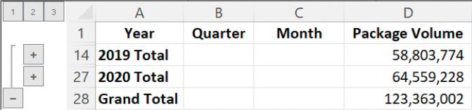
The data range with details hidden at level 2
You can add custom levels of detail to the outline that Excel creates by grouping specific rows. (For example, you can hide revenues from specific months.) You can also delete groups you don’t need and remove the subtotals and outlining entirely.
To organize data into levels
Sort the data range, ensuring that the top-level sort is on the column by which you want to group the data.
Select the data range you want to sort or a cell in the range.
On the Data tab, in the Outline group, select the Subtotal button.
In the Subtotal dialog, in the At each change in list, select the field by which you want to group the data.
 Important
You must first sort the data by the field that you plan to summarize by selecting the Subtotal button.
In the Use function list, select the summary function you want to use for each subtotal.
In the Add subtotal to group, select the checkbox next to any field you want to summarize. Then select OK.
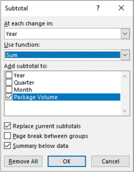
Apply subtotals to data from the Subtotal dialog
To show or hide detail in an outlined range
To hide or show one group, select its Hide Detail (+) or Show Detail (–) control.
To hide or show one level, select the level button.
To create a custom group in an outlined range
Select the rows you want to include in the group.
On the Data tab, in the Outline group, select the Group button (not the arrow).
A custom group within an outline
To remove a custom group from an outlined range
Select the rows you want to remove from the group.
On the Data tab, in the Outline group, select the Ungroup button (not the arrow).
To remove subtotals from a data range
Select any cell in the range.
On the Data tab, in the Outline group, select Subtotal.
In the Subtotal dialog, select Remove All.
Key points
You can sort the data in a range or table by the values in one or multiple columns. Excel discerns the basic sort order (A to Z, small to large, old to new) based on the data in the column. You can also sort data to bring a single cell color, font color, or icon to the top.
If the default sort orders don’t meet your needs, you can provide Excel with a list by which it should sort. Custom lists with the days of the week and months of the year in order of occurrence are built in to Excel, but you can make up your own.
You can outline, group, and subtotal data by using the Subtotal feature (which is different from the SUBTOTAL function). To successfully subtotal data, you must first sort it by the column that will define the data groups.
![]() See Also
See Also
This chapter is from the full-length book Microsoft Excel Step by Step (Office 2021 and Microsoft 365) (Microsoft Press, 2021). Please consult that book for information about features of Excel that aren’t discussed in this book.
Practice tasks

Before you can complete these tasks, you must copy the book’s practice files to your computer. The practice files for these tasks are in the Office365SBSCh08 folder. You can save the results of the tasks in the same folder.
The introduction includes a complete list of practice files and download instructions.
Sort worksheet data
Open the SortData workbook in Excel, and then perform the following tasks:
Sort the data in the cell range B3:D14 in ascending order by the values in the Revenue column.
Sort the data range in descending order by the values in the Revenue column.
Perform a two-level sort of the data range:
In ascending order by Customer.
In ascending order by Season.
Review the effect of the multiple-column sort. Be sure that you understand the effect of the sort operation order.
Reverse the order of the fields in the Sort dialog to sort first by Season and then by Customer.
Sort the data range by the Revenue column so that the cells that have a red fill color are at the top of the list.
Save and close the file.
Sort data by using custom lists
Open the CustomSortData workbook in Excel, and then perform the following tasks:
Create a custom list by using the values in cells G4:G7.
Sort the data in the cell range B2:D14 by the Season column based on the custom list you just created.
Perform a two-level sort of the data range:
By Customer in ascending order.
By Season in the custom list order.
Save and close the file.
Outline and subtotal data
Open the OutlineData workbook in Excel, and then perform the following tasks:
Outline the data list in cells A1:D25 to find the subtotal for each year.
Hide the details of rows for the year 2020.
Create a new group consisting of the rows showing data for June and July 2019.
Hide the details of the group you just created.
Show the details of all months for the year 2020.
Remove the subtotal outline from the entire data list.
Save and close the file.