
9
Analyze alternative data sets
In this chapter
When you store data in an Excel workbook, you can use that data, either by itself or as part of a calculation, to discover important information about your organization.
The data in your worksheets is great for answering “what-if” questions, such as “How much money would we save if we reduced our labor to 20 percent of our total costs?” You can always save an alternative version of a workbook and create formulas that calculate the effects of your changes, but you can do the same thing in your existing workbooks by defining one or more alternative data sets. You can also create a data table that calculates the effects of changing one or two variables in a formula, find the input values required to generate the result you want, and describe your data statistically.
This chapter guides you through procedures related to defining scenarios that result in alternative data sets, forecasting data by using data tables, and using Goal Seek to identify the input necessary to achieve a specific result.
Define and display alternative data sets
When you save data in an Excel worksheet, you create a record that reflects the characteristics of an event or object. For example, that data could represent the number of deliveries in an hour on a specific day, the price of a new delivery option, the percentage of total revenue accounted for by a delivery option—the possibilities are endless. After the data is in place, you can create formulas to generate totals, find averages, and sort the rows in a worksheet based on the contents of one or more columns. However, if you want to perform a what-if analysis or explore the impact that changes in the data would have on any of the calculations in your workbooks, you must change the data. By doing so, you run the risk of losing the original data. If you only want to make temporary changes for forecasting purposes, you can safely do so by applying a scenario—a set of alternative values—to the original data set to create an alternative data set.
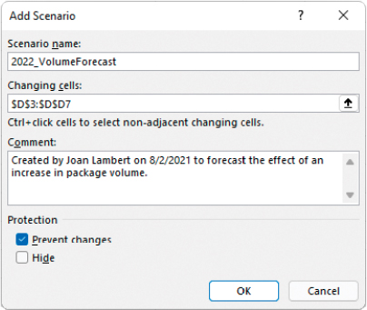
A scenario changes data in specific cells
Applying a scenario creates an alternative data set by replacing the values in the original data set with the alternative values defined in the scenario and recalculating any formulas that depend on those values. After you apply the scenario, you can return to the original data set by undoing the scenario.
![]() Important
Important
It's important to revert to the original data set before you save and close the workbook, because the original data isn’t stored anywhere. To avoid accidentally losing the original data, create a scenario that contains the original values or create a scenario summary.
Each scenario can change a maximum of 32 cells, so if you want to modify a lot of data, you will need to create multiple scenarios. You can create and apply as many scenarios as you want. (If multiple scenarios affect the same cell, the cell displays the value created by the most recently applied scenario.)
If you want to keep a record of the effect of various scenarios within a workbook, you can create a scenario summary worksheet that displays the effect of the scenarios on specific cells.
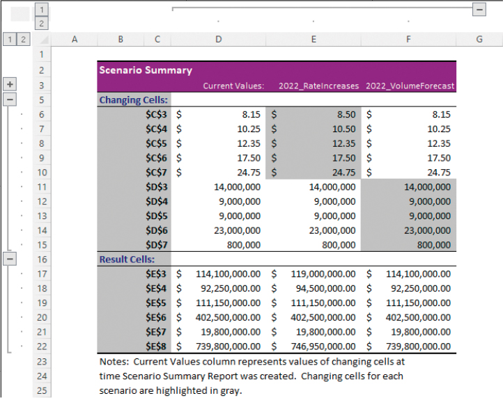
A scenario summary worksheet tracks the effects of all scenarios
As with other Excel tools, you can edit and delete the scenarios you create. Deleting a scenario does not undo the effects of the scenario on the worksheet data; it only removes the scenario from the Scenario Manager dialog.
To open the Scenario Manager dialog
On the Data tab, in the Forecast group, select What-If Analysis, and then select Scenario Manager.
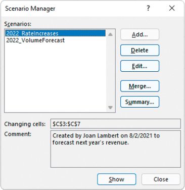
Manage and summarize scenarios
To define a scenario
Open the Scenario Manager dialog.
Select Add.
In the Add Scenario dialog, enter a name for the scenario in the Scenario name box.
Do either of the following:
In the Changing cells box, enter the cell references of the cell values you want to change.
Activate the Changing cells box and then, on the worksheet, select the cells in which you want to change the values.
 Tip
TipWhen you select the cells on the worksheet, the dialog name changes from Add Scenario to Edit Scenario.
In the Comment box that contains your name and the date, append any notes that you might find useful later.
In the Add Scenario dialog, select OK.
In the Scenario Values dialog, replace the original values of each of the changing cells, and then select OK.
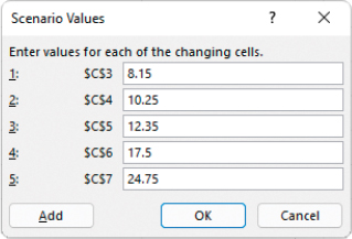
Enter alternative data in the Scenario Values dialog
To display an alternative data set
In the Scenario Manager dialog, select the scenario you want to apply, and then select Show.
To apply additional scenarios, repeat step 1.
To revert to the original data set
Close the Scenario Manager dialog, and then do either of the following:
On the Quick Access Toolbar, select the Undo button.
Press Ctrl+Z.
To edit a scenario
In the Scenario Manager dialog, select the scenario you want to edit, and then select Edit.
In the Edit Scenario dialog, change any values in the Scenario name, Changing cells, or Comment boxes, and then select OK.
In the Scenario Values dialog, modify the new values for the changing cells, and then select OK.
To delete a scenario
In the Scenario Manager dialog, select the scenario you want to delete, and then select Delete.
To create a scenario summary worksheet
Revert any scenarios that have been applied to the original data set.
 Important
Make sure there are no scenarios applied to the workbook when you create the summary worksheet. If a scenario is active, Excel will record the alternative data set as the original values, and the summary will be inaccurate.
In the Scenario Manager dialog, select Summary.
In the Scenario Summary dialog, select Scenario summary.
Do either of the following:
In the Result cells box, enter the cell references of the cell changes you want to summarize.
Activate the Result cells box and then, on the worksheet, select the cells whose changes you want to summarize.
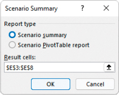
Summarize scenarios by using the Scenario Summary dialog
In the Scenario Summary dialog, select OK.
Forecast data by using data tables
Data tables are another useful data-forecasting tool in Excel. They let you clearly see the result of applying different patterns to existing data

Projecting different rates of increase on the current data
A data table can forecast changes to either one or two formula inputs. These are called the variables. To create a data table with one variable, you arrange the formula inputs—including the changing value, the variable values, and a summary formula—on a worksheet, leaving an area for the data table in the lower-right corner of the cell range. The variable values can be in a column (as shown here) or in a row.
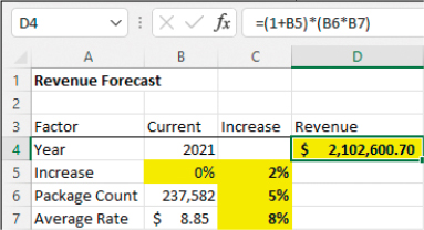
Excel substitutes the variables for the changing value
In the example shown above, the formula inputs are in B5:B7, with the changing value in B5, the variables in C5:C7, and the summary formula (shown in the formula bar) in cell D4. Excel builds the data table in D5:D7 to reflect the effect of the variables on the summary formula.
To create a two-variable data table, arrange the formula inputs, including the two changing values, in the same way as for the one-variable table. Place one set of variable values in a column and another in a row, again leaving an area for the data table in the lower-right corner. Place the summary formula at the junction of the column and the row.
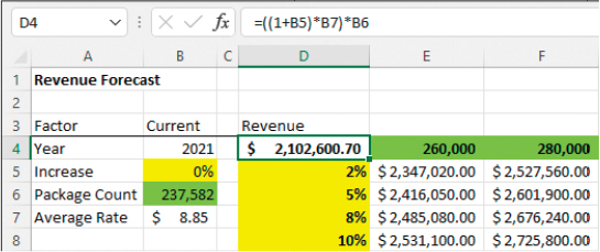
Two-variable data tables generate multiple outcomes
In this example, the variables in D5:D8 represent the rate increase and the variables in E4:F4 represent the package count increase.
To create a one-variable data table
On a worksheet, enter the following information, and arrange it as shown and described above:
A summary formula
The input values for the summary formula
A column (or row) of alternative values for one of the input values
Select the cells representing the variables and the summary formula, and the cells in which the data table displaying the alternative formula results should appear.
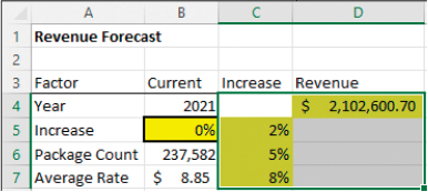
Identify the input and output cells for the data table
On the Data tab, in the Forecast group, select What-If Analysis, and then select Data Table.
In the Data Table dialog, do either of the following:
If the variables are in a row, enter the cell reference of the changing value in the Row input cell box.
If the variables are in a column, enter the cell reference of the changing value in the Column input cell box.
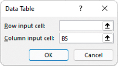
Identify the changing value
Select OK.
To create a two-variable data table
On a worksheet, enter the following information, and arrange it as shown and described above:
A summary formula
The input values for the summary formula
A column of alternative values for one input value
A row of alternative values for another input value
Select the cells representing the variables and the summary formula, and the cells in which the data table displaying the alternative formula results should appear.
On the What-If Analysis menu, select Data Table.
In the Data Table dialog, in the Row input cell box, enter the cell reference of the cell whose alternative values are in a row.
In the Column input cell box, enter the cell reference of the cell whose alternative values are in a column.
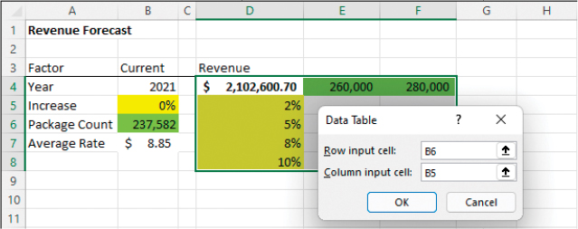
Identify both changing values
Select OK.
Identify the input necessary to achieve a specific result
When you run an organization, you must track how every element performs, both in absolute terms and in relation to other parts of the organization. There are many ways to measure your operations, but one useful technique is to limit the percentage of total costs contributed by a specific item.
As an example, consider a worksheet that displays the actual costs and percentage of total costs for several production input values.
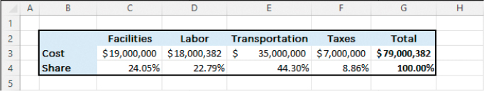
A worksheet that contains formulas that calculate the percentage of total costs for each of four categories
Under the current pricing structure, transportation represents 44.3 percent of the total cost of creating the product. If you want to get the transportation costs below 35 percent of the total, you can manually change the cost until you find the number you want. Alternatively, you can use Excel’s Goal Seek feature to find the solution for you. You simply tell Goal Seek your target value for the cell and the value you want to change to get there.
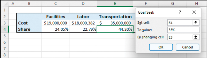
Identify the cell that contains the formula you want to use to generate a target value
Goal Seek finds the closest solution it can without exceeding the target you set and provides a suggested value. You can accept the suggestion to replace the original value or reject it to revert to the original value.
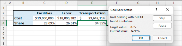
A worksheet in which Goal Seek found a solution to a problem
To find a target value by using Goal Seek
On the Data tab, in the Forecast group, select What-If Analysis, and then select Goal Seek.
In the Goal Seek dialog, in the Set cell box, enter the cell whose value you want to change.
In the To value box, enter the target value for the cell.
In the By changing cell box, enter the cell that contains the value you want to vary to produce the result you want.
Select OK.
![]() Important
Important
Saving a workbook with the results of a Goal Seek calculation in place overwrites the original workbook values. Consider running Goal Seek calculations on copies of the original data or reverting calculations immediately so you don't accidentally save or autosave them.
Key points
In the Scenario Manager, you can forecast the effect of changing data within a data range or table without actually making the changes and possibly losing track of your original data. You can save the results of various scenarios in a scenario summary worksheet.
Another way to forecast data is in a data table, which shows the effect on a formula of changing either one or two variables.
If you know the specific result that you need to achieve with a formula, you can use the Goal Seek feature to identify the necessary input values.
![]() See Also
See Also
This chapter is from the full-length book Microsoft Excel Step by Step (Office 2021 and Microsoft 365) (Microsoft Press, 2021). Please consult that book for information about features of Excel that aren’t discussed in this book.
Practice tasks

Before you can complete these tasks, you must copy the book’s practice files to your computer. The practice files for these tasks are in the Office365SBSCh09 folder. You can save the results of the tasks in the same folder.
The introduction includes a complete list of practice files and download instructions.
Define and display alternative data sets
Open the CreateScenarios workbook in Excel, and then perform the following tasks:
Create a scenario named Overnight that changes the Base Rate value for Overnight and Priority Overnight packages (in cells C6 and C7) to $18.75 and $25.50.
Apply the Overnight scenario and note its effects on the data.
Press Ctrl+Z to revert to the original data.
Create a scenario named HighVolume that increases the number of Ground packages to 17,000,000 and 3-Day packages to 14,000,000.
Create a scenario named NewRates that increases the Ground rate to $9.45 and the 3-Day rate to $12.
Create a scenario summary worksheet that displays the effects of the three scenarios.
Apply the HighVolume scenario and note its effects on the data.
Apply the NewRates scenario and note the additional changes.
Forecast data by using data tables
Open the DefineDataTables workbook in Excel, and then perform the following tasks:
On the RateIncreases worksheet, select cells C4:D7.
Perform the steps to create a data table in cells D5:D7, entering B5 as the Column input cell. Review the resulting data.
On the RateAndVolume worksheet, select cells D4:F8.
Perform the steps to create a data table in cells E5:F8, entering B6 as the Row input cell and B5 as the Column input cell. Review the resulting data.
Identify the input necessary to achieve a specific result
Open the PerformGoalSeekAnalysis workbook in Excel, and then perform the following tasks:
Select cell C4.
Open the Goal Seek dialog.
Verify that C4 appears in the Set cell box.
In the To value box, enter 20%.
In the By changing cell box, enter C3.
Select OK.