
1
Pandas DataFrame Basics
1.1 Introduction
Pandas is an open-source Python library for data analysis. It gives Python the ability to work with spreadsheet-like data for fast data loading, manipulating, aligning, merging, etc. To give Python these enhanced features, Pandas introduces two new data types to Python: Series and DataFrame. The DataFrame will represent your entire spreadsheet or rectangular data, whereas the Series is a single column of the DataFrame. A Pandas DataFrame can also be thought of as a dictionary or collection of Series.
Why should you use a programming language like Python and a tool like Pandas to work with data? It boils down to automation and reproducibility. If there is a particular set of analyses that needs to be performed on multiple data sets, a programming language can automate the analysis on the data sets. Although many spreadsheet programs have their own macro programming languages, many users do not use them. Furthermore, not all spreadsheet programs are available on all operating systems. Performing data tasks using a programming language forces the user to have a running record of all steps performed on the data. I, like many people, have accidentally hit a key while viewing data in a spreadsheet program, only to find out that my results do not make any sense anymore due to bad data. This is not to say spreadsheet programs are bad or do not have their place in the data workflow. They do, but there are better and more reliable tools out there. These better tools can work in tandem with spreadsheet programs while providing more reliable data manipulation, and introduce the possibility of incorporating data from other data sets and databases.
Learning Objectives
The concept map for this chapter can be found in Figure A.1.
Use Pandas functions to load a simple delimited data file
Calculate how many rows and columns were loaded
Identify the type of data that were loaded
Name differences between functions, methods, and attributes
Use methods and attributes to subset rows and columns
Calculate basic grouped and aggregated statistics from data
Use methods and attributes to create a simple figure from data
1.2 Load Your First Data Set
When given a data set, we first load it and begin looking at its structure and contents. The simplest way of looking at a data set is to look at and subset specific rows and columns. We can see what type of information is stored in each column, and can start looking for patterns by aggregating descriptive statistics.
Since Pandas is not part of the Python standard library, we have to first tell Python to load (i.e., import) the library. If you have not installed data and packages needed to go through the book please see Appendix B.
import pandasWith the library loaded we can use the read_csv() function to load a CSV data file. In order to access the read_csv() function from pandas, we use something called “dot notation.” More on dot notations can be found in Appendix L, Appendix P, and Appendix E. We write pandas.read_csv() to say: within the pandas library we just loaded, look inside for the read_csv() function.
# by default read_csv() will read a comma separated file,
# our gapminder data set is separated by a tab
# we can use the sep parameter and indicate a tab with
df  = pandas.read_csv('./data/gapminder.tsv', sep='	')
# print out the data
print(df)
country continent year lifeExp pop gdpPercap
0 Afghanistan Asia 1952 28.801 8425333 779.445314
1 Afghanistan Asia 1957 30.332 9240934 820.853030
2 Afghanistan Asia 1962 31.997 10267083 853.100710
3 Afghanistan Asia 1967 34.020 11537966 836.197138
4 Afghanistan Asia 1972 36.088 13079460 739.981106
... ... ... ... ... ... ...
1699 Zimbabwe Africa 1987 62.351 9216418 706.157306
1700 Zimbabwe Africa 1992 60.377 10704340 693.420786
1701 Zimbabwe Africa 1997 46.809 11404948 792.449960
1702 Zimbabwe Africa 2002 39.989 11926563 672.038623
1703 Zimbabwe Africa 2007 43.487 12311143 469.709298
[1704 rows x 6 columns]Since we will be using Pandas functions many times throughout the book as well as in your own programming. It is common to give pandas the alias pd. The above code will be the same as below:
import pandas as pd
df = pd.read_csv('./data/gapminder.tsv', sep='	')
We can check to see if we are working with a Pandas Dataframe by using the built-in type() function (i.e., it comes directly from Python, not a separate library such as Pandas).
print(type(df))<class 'pandas.core.frame.DataFrame'>The type() function is handy when you begin working with many different types of Python objects and need to know what object you are currently working on.
The data set we loaded is currently saved as a Pandas DataFrame object (pandas.core.frame.DataFrame) and is relatively small. Every DataFrame object has a .shape attribute that will give us the number of rows and columns of the DataFrame.
# get the number of rows and columns
print(df.shape)
(1704, 6)The shape attribute returns a tuple (Appendix G) where the first value is the number of rows and the second value is the number of columns.
From the results above, we see our gapminder data set has 1704 rows and 6 columns.
Since .shape is an attribute of the DataFrame object, and not a function or method of the DataFrame object, it does not have round parentheses after the period (i.e., it’s written as df.shape and not df.shape()). If you made the mistake of putting parentheses after the .shape attribute, it would return an error.
# shape is an attribute, not a method
# this will cause an error
print(df.shape())
TypeError: 'tuple' object is not callableTypically, when first looking at a data set, we want to know how many rows and columns there are (we just did that). To get a gist of what information the data set contains, we look at the column names. The column names, like .shape, are given using the .column attribute of the DataFrame object.
# get column names
print(df.columns)
Index(['country', 'continent', 'year', 'lifeExp', 'pop',
'gdpPercap'],
dtype='object')The Pandas DataFrame object is similar to other languages that have DataFrame-like objects (e.g., Julia and R). Each column (i.e., Series) has to be the same type, whereas each row can contain mixed types. In our current example, we can expect the country column to be all strings, and the year to be integers. However, it’s best to make sure that is the case by using the .dtypes attribute or the .info() method. Table 1.1 shows what the type in Pandas is relative to native Python.
# get the dtype of each column
print(df.dtypes)
country object
continent object
year int64
lifeExp float64
pop int64
gdpPercap float64
dtype: object# get more information about our data
print(df.info())<class 'pandas.core.frame.DataFrame'>
RangeIndex: 1704 entries, 0 to 1703
Data columns (total 6 columns):
# Column Non-Null Count Dtype
--- ------ -------------- -----
0 country 1704 non-null object
1 continent 1704 non-null object
2 year 1704 non-null int64
3 lifeExp 1704 non-null float64
4 pop 1704 non-null int64
5 gdpPercap 1704 non-null float64
dtypes: float64(2), int64(2), object(2)
memory usage: 80.0+ KB
None1.3 Look at Columns, Rows, and Cells
Now that we’re able to load up a simple data file, we want to be able to inspect its contents. We could print() out the contents of the DataFrame, but with today’s data, there are too many cells to make sense of all the printed information. Instead, the best way to look at our data is to inspect it by looking at various subsets of the data. We can use the .head() method of a DataFrame to look at the first 5 rows of our data.
Table 1.1 Table of Pandas dtypes and Python Types
Pandas | Python | Description |
|---|---|---|
object | string | most common data type |
int64 | int | whole numbers |
float64 | float | numbers with decimals |
datetime64 | datetime | datetime is found in the Python standard library (i.e., it is not loaded by default and needs to be imported) |
# show the first 5 observations
print(df.head())
country continent year lifeExp pop gdpPercap
0 Afghanistan Asia 1952 28.801 8425333 779.445314
1 Afghanistan Asia 1957 30.332 9240934 820.853030
2 Afghanistan Asia 1962 31.997 10267083 853.100710
3 Afghanistan Asia 1967 34.020 11537966 836.197138
4 Afghanistan Asia 1972 36.088 13079460 739.981106This is useful to see if our data loaded properly, and to get a better sense of the columns and contents. However, there are going to be times when we only want particular rows, columns, or values from our data.
Before continuing, make sure you are familiar with Python containers (Appendix F, Appendix H).
1.3.1 Select and Subset Columns by Name
If we want only a specific column from our data, we can access the data using square brackets, [ ].
# just get the country column and save it to its own variable
country_df = df['country']# show the first 5 observations
print(country_df.head())0 Afghanistan
1 Afghanistan
2 Afghanistan
3 Afghanistan
4 Afghanistan
Name: country, dtype: object# show the last 5 observations
print(country_df.tail())
1699    Zimbabwe
1700    Zimbabwe
1701    Zimbabwe
1702    Zimbabwe
1703    Zimbabwe
Name: country, dtype: object
In order to specify multiple columns by the column name, we need to pass in a Python list between the square brackets. This may look a bit strange since there will be 2 sets of square brackets, [[ ]].
The outer set of square brackets tells us that we are subsetting our DataFrame by columns. The inner set of square brackets tells us the list of columns we want to use. That is, Python also uses square brackets, [ ], to “list” multiple things as a single object.
# Looking at country, continent, and year
subset = df[['country', 'continent', 'year']]print(subset) country continent year
0 Afghanistan Asia 1952
1 Afghanistan Asia 1957
2 Afghanistan Asia 1962
3 Afghanistan Asia 1967
4 Afghanistan Asia 1972
... ... ... ...
1699 Zimbabwe Africa 1987
1700 Zimbabwe Africa 1992
1701 Zimbabwe Africa 1997
1702 Zimbabwe Africa 2002
1703 Zimbabwe Africa 2007
[1704 rows x 3 columns]Using the square bracket notation, [ ], you cannot pass an index position to subset a DataFrame based on the position of the columns. If you want to do this, look down for the .iloc[] notation.
# subset the first column based on its position.
df[0]
KeyError: 01.3.1.1 Single Value Returns DataFrame or Series
When we first selected a single column we were given a Series object back.
country_df = df['country']
print(type(country_df))
<class 'pandas.core.series.Series'>We can also tell it’s a Series because it prints out slightly differently from the DataFrame.
print(country_df)0 Afghanistan
1 Afghanistan
2 Afghanistan
3 Afghanistan
4 Afghanistan
...
1699 Zimbabwe
1700 Zimbabwe
1701 Zimbabwe
1702 Zimbabwe
1703 Zimbabwe
Name: country, Length: 1704, dtype: objectCompare those results to passing in a single element list (note the double square bracket, [[ ]]):
country_df_list = df[['country']] # note the double square bracket
print(type(country_df_list))
<class 'pandas.core.frame.DataFrame'>If we use a list to subset, we will always get a DataFrame object back.
print(country_df_list) country
0 Afghanistan
1 Afghanistan
2 Afghanistan
3 Afghanistan
4 Afghanistan
... ...
1699 Zimbabwe
1700 Zimbabwe
1701 Zimbabwe
1702 Zimbabwe
1703 Zimbabwe
[1704 rows x 1 columns]Depending on what you need, sometimes you only need a single Series (sometimes called a vector), other times for consistency, you will want a DataFrame object.
1.3.1.2 Using Dot Notation to Pull a Column of Values
When all you need is a single column (i.e., Series or vector) of values and typing df['column'] will be very tedious. There is a shorthand notation where you can pull the column vector by treating it as a DataFrame attribute.
For example, below are two ways of returning the same single column Series.
# using square bracket notation
print(df['country'])
0 Afghanistan
1 Afghanistan
2 Afghanistan
3 Afghanistan
4 Afghanistan
...
1699 Zimbabwe
1700 Zimbabwe
1701 Zimbabwe
1702 Zimbabwe
1703 Zimbabwe
Name: country, Length: 1704, dtype: object# using dot notation
print(df.country)0 Afghanistan
1 Afghanistan
2 Afghanistan
3 Afghanistan
4 Afghanistan
...
1699 Zimbabwe
1700 Zimbabwe
1701 Zimbabwe
1702 Zimbabwe
1703 Zimbabwe
Name: country, Length: 1704, dtype: objectThere are subtle differences if you want to do other operations (e.g., deleting a column), but for now, you can treat those 2 ways of getting a single column of values as the same. You do have to be mindful of what your columns are named if you want to use the dot notation. That is, if there is a column named shape, the df.shape will return the number of rows and columns from the .shape attribute, not the intended shape column. Also, if your column name has spaces or special characters, you will not be able to use the dot notation to select that column of values, and will have to use the square bracket notation.
1.3.2 Subset Rows
Rows can be subset in multiple ways, by row name or row index. Table 1.2 gives a quick overview of the various methods.
Table 1.2 Different Methods of Indexing Rows (and/or Columns)a
Subset attribute | Description |
|---|---|
| Subset based on index label (row name) |
| Subset based on row index (row number) |
|
|
a Subsetting data with .ix[] is no longer supported in Pandas. The reason why .ix[] was removed is because it would first match on the index label, and if the value was not found, it would match on the index position. This dual subsetting behavior was not explicit and could be problematic since you did not always know how it was subsetting your rows.
1.3.2.1 Subset Rows by index Label - .loc[]
If we take a look at our gapminder data:
print(df) country continent year lifeExp pop gdpPercap
0 Afghanistan Asia 1952 28.801 8425333 779.445314
1 Afghanistan Asia 1957 30.332 9240934 820.853030
2 Afghanistan Asia 1962 31.997 10267083 853.100710
3 Afghanistan Asia 1967 34.020 11537966 836.197138
4 Afghanistan Asia 1972 36.088 13079460 739.981106
... ... ... ... ... ... ...
1699 Zimbabwe Africa 1987 62.351 9216418 706.157306
1700 Zimbabwe Africa 1992 60.377 10704340 693.420786
1701 Zimbabwe Africa 1997 46.809 11404948 792.449960
1702 Zimbabwe Africa 2002 39.989 11926563 672.038623
1703 Zimbabwe Africa 2007 43.487 12311143 469.709298
[1704 rows x 6 columns]We can see on the left side of the printed DataFrame, what appear to be row numbers. This column-less row of values is the “index” label of the DataFrame. Think of it like column names, but, for rows. By default, Pandas will fill in the index labels with the row numbers (note that it starts counting from 0). A common example where the row index labels are not the row number is when we work with time series data. In that case, the index label will be a timestamp, but for now, we will keep the default row number values.
We can use the .loc[] accessor attribute on the DataFrame to subset rows based on the index label.
# get the first row
# python counts from 0
print(df.loc[0])
country       Afghanistan
continent            Asia
year                 1952
lifeExp            28.801
pop               8425333
gdpPercap      779.445314
Name: 0, dtype: object# get the 100th row
# python counts from 0
print(df.loc[99])country Bangladesh
continent Asia
year 1967
lifeExp 43.453
pop 62821884
gdpPercap 721.186086
Name: 99, dtype: object# get the last row
# this will cause an error
print(df.loc[-1])KeyError: -1Note that passing -1 as the .loc[] will cause an error because it is actually looking for the row index label (i.e., row number) -1, which does not exist in our example DataFrame. Instead, we can use a bit of Python to calculate the total number of rows, and then pass that value into .loc[].
# get the last row (correctly)

# use the first value given from shape to get the number of rows
number_of_rows = df.shape[0]

# subtract 1 from the value since we want the last index value
last_row_index = number_of_rows - 1

# finally do the subset using the index of the last row
print(df.loc[last_row_index])
country Zimbabwe
continent Africa
year 2007
lifeExp 43.487
pop 12311143
gdpPercap 469.709298
Name: 1703, dtype: objectOr use the .tail() method to return the last n=1 row, instead of the default 5.
# there are many ways of doing what you want
print(df.tail(n=1))
country continent year lifeExp pop gdpPercap
1703 Zimbabwe Africa 2007 43.487 12311143 469.709298Notice that using .tail() and .loc[] printed out the results differently. Let’s look at what type is returned when we use these methods.
# get the last row of data in different ways
subset_loc = df.loc[0]
subset_head = df.head(n=1)
# type using loc of 1 row
print(type(subset_loc))<class 'pandas.core.series.Series'># type of using head of 1 row
print(type(subset_head))<class 'pandas.core.frame.DataFrame'>At the beginning of this chapter, we mentioned that Pandas introduces two new data types into Python: Series and DataFrame. Depending on which method we use and how many rows we return, Pandas will return a different object. The way an object gets printed to the screen can be an indicator of the type, but it’s always best to use the type() function to be sure. We go into more detail about these objects in Chapter 2.
1.3.2.2 Subsetting Multiple Rows
As with columns, we can filter multiple rows.
print(df.loc[[0, 99, 999]]) country continent year lifeExp pop gdpPercap
0 Afghanistan Asia 1952 28.801 8425333 779.445314
99 Bangladesh Asia 1967 43.453 62821884 721.186086
999 Mongolia Asia 1967 51.253 1149500 1226.0411301.3.3 Subset Rows by Row Number: .iloc[]
.iloc[] does the same thing as .loc[], but is used to subset by the row index number. In our current example, .iloc[] and .locp[] will behave exactly the same way since the index labels are the row numbers. However, keep in mind that the index labels do not necessarily have to be row numbers.
# get the 2nd row
print(df.iloc[1])
country Afghanistan
continent Asia
year 1957
lifeExp 30.332
pop 9240934
gdpPercap 820.85303
Name: 1, dtype: object## get the 100th row
print(df.iloc[99])country Bangladesh
continent Asia
year 1967
lifeExp 43.453
pop 62821884
gdpPercap 721.186086
Name: 99, dtype: objectNote that when we subset on 1, we actually get the second row, rather than the first row. This follows Python’s zero-indexed behavior, meaning that the first item of a container is index 0 (i.e., 0th item of the container). More details about this kind of behavior are found in Appendix F, Appendix I, and Appendix M.
With .iloc[], we can pass in the -1 to get the last row — something we couldn’t do with .loc[].
# using -1 to get the last row
print(df.iloc[-1])
country Zimbabwe
continent Africa
year 2007
lifeExp 43.487
pop 12311143
gdpPercap 469.709298
Name: 1703, dtype: objectJust as before, we can pass in a list of integers to get multiple rows.
## get the first, 100th, and 1000th row
print(df.iloc[[0, 99, 999]])
country continent year lifeExp pop gdpPercap
0 Afghanistan Asia 1952 28.801 8425333 779.445314
99 Bangladesh Asia 1967 43.453 62821884 721.186086
999 Mongolia Asia 1967 51.253 1149500 1226.0411301.3.4 Mix It Up
We can use .loc[] and .iloc[] to obtain subsets rows, columns, or both. The general syntax for .loc[] and .iloc[] uses square brackets with a comma. The part to the left of the comma is the row values to subset; the part to the right of the comma is the column values to subset. That is, df.loc[[rows], [columns]] or df.iloc[[rows], [columns]].
1.3.4.1 Selecting Columns
If we want to use these techniques to just subset columns, we must use Python’s slicing syntax (Appendix I). We need to do this because if we are subsetting columns, we are getting all the rows for the specified column. So, we need a method to capture all the rows.
The Python slicing syntax uses a colon, :. If we have just a colon, it “slices” (i.e., gets) all the values in that axis. So, if we just want to get the first column using the .loc[] or .iloc[] syntax, we can write df.loc[:, [columns]] to subset the column(s).
# subset columns with loc
# note the position of the colon
# it is used to select all rows
subset = df.loc[:, ['year', 'pop']]
print(subset)
year pop
0 1952 8425333
1 1957 9240934
2 1962 10267083
3 1967 11537966
4 1972 13079460
... ... ...
1699 1987 9216418
1700 1992 10704340
1701 1997 11404948
1702 2002 11926563
1703 2007 12311143
[1704 rows x 2 columns]# subset columns with iloc
# iloc will allow us to use integers
# -1 will select the last column
subset = df.iloc[:, [2, 4, -1]]
print(subset) year pop gdpPercap
0 1952 8425333 779.445314
1 1957 9240934 820.853030
2 1962 10267083 853.100710
3 1967 11537966 836.197138
4 1972 13079460 739.981106
... ... ... ...
1699 1987 9216418 706.157306
1700 1992 10704340 693.420786
1701 1997 11404948 792.449960
1702 2002 11926563 672.038623
1703 2007 12311143 469.709298
[1704 rows x 3 columns]We will get an error if we don’t specify .loc[] or iloc[] correctly.
# subset columns with loc
# but pass in integer values
# this will cause an error
subset = df.loc[:, [2, 4, -1]]
print(subset)
KeyError: "None of [Int64Index([2, 4, -1], dtype='int64')]
are in the [columns]"# subset columns with iloc
# but pass in index names
# this will cause an error
subset = df.iloc[:, ['year', 'pop']]
print(subset)IndexError: .iloc requires numeric indexers, got ['year' 'pop']1.3.4.2 Subsetting with range()
You can use the built-in range() function to create a range of values in Python. This way you can specify beginning and end values, and Python will automatically create a range of values in between. By default, every value between the beginning and the end (inclusive left, exclusive right; see Appendix I) will be created, unless you specify a step (Appendix I and Appendix M). In Python 3, the range() function returns a generator. A generator is like a single-use list; it disappears after you use it once. This is mainly to save system resources. See Appendix M for more information about generators.
We just saw in Section 1.3.4.1 how we can select columns using a list of integers. Since range() returns a generator, we have to first convert the generator to a list.
# create a range of integers from 0 - 4 inclusive
small_range = list(range(5))
print(small_range)
[0, 1, 2, 3, 4]# subset the dataframe with the range
subset = df.iloc[:, small_range]
print(subset)
         country continent  year  lifeExp       pop
0    Afghanistan      Asia  1952   28.801   8425333
1    Afghanistan      Asia  1957   30.332   9240934
2    Afghanistan      Asia  1962   31.997  10267083
3    Afghanistan      Asia  1967   34.020  11537966
4    Afghanistan      Asia  1972   36.088  13079460
...          ...       ...   ...      ...       ...
1699    Zimbabwe    Africa  1987   62.351   9216418
1700    Zimbabwe    Africa  1992   60.377  10704340
1701    Zimbabwe    Africa  1997   46.809  11404948
1702    Zimbabwe    Africa  2002   39.989  11926563
1703    Zimbabwe    Africa  2007   43.487  12311143
[1704 rows x 5 columns]Note that when list(range(5)) is called, five integers are returned: 0 – 4.
# create a range from 3 - 5 inclusive
small_range = list(range(3, 6))
print(small_range)
[3, 4, 5]subset = df.iloc[:, small_range]
print(subset) lifeExp pop gdpPercap
0 28.801 8425333 779.445314
1 30.332 9240934 820.853030
2 31.997 10267083 853.100710
3 34.020 11537966 836.197138
4 36.088 13079460 739.981106
... ... ... ...
1699 62.351 9216418 706.157306
1700 60.377 10704340 693.420786
1701 46.809 11404948 792.449960
1702 39.989 11926563 672.038623
1703 43.487 12311143 469.709298[1704 rows x 3 columns]Again, note that the values are specified in a way such that the range is inclusive on the left, and exclusive on the right.
We can also pass in a 3rd parameter into range, step, that allows us to change how to increment between the start and stop values (defaults to step=1).
# create a range from 0 - 5 inclusive, every other integer
small_range = list(range(0, 6, 2))
subset = df.iloc[:, small_range]
print(subset) country year pop
0 Afghanistan 1952 8425333
1 Afghanistan 1957 9240934
2 Afghanistan 1962 10267083
3 Afghanistan 1967 11537966
4 Afghanistan 1972 13079460
... ... ... ...
1699 Zimbabwe 1987 9216418
1700 Zimbabwe 1992 10704340
1701 Zimbabwe 1997 11404948
1702 Zimbabwe 2002 11926563
1703 Zimbabwe 2007 12311143[1704 rows x 3 columns]Converting a generator to a list is a bit awkward; we can use the Python slicing syntax to fix this.
1.3.4.3 Subsetting with Slicing :
Python’s slicing syntax, :, is similar to the range() function. Instead of a function that specifies start, stop, and step values delimited by a comma, we separate the values with the colon, :.
If you understand what was going on with the range() function earlier, then slicing can be seen as a shorthand for the same thing.
The range() function can be used to create a generator that can also be converted to a list of values. The colon syntax, :, only has meaning within the square bracket, [ ] slicing and subsetting context; it has no inherent meaning on its own.
Here are the columns of our data set.
print(df.columns)Index(['country', 'continent', 'year', 'lifeExp', 'pop',
'gdpPercap'],
dtype='object')See how range() and : are used to slice our data.
small_range = list(range(3))
subset = df.iloc[:, small_range]
print(subset)
country continent year
0 Afghanistan Asia 1952
1 Afghanistan Asia 1957
2 Afghanistan Asia 1962
3 Afghanistan Asia 1967
4 Afghanistan Asia 1972
... ... ... ...
1699 Zimbabwe Africa 1987
1700 Zimbabwe Africa 1992
1701 Zimbabwe Africa 1997
1702 Zimbabwe Africa 2002
1703 Zimbabwe Africa 2007[1704 rows x 3 columns]# slice the first 3 columns
subset = df.iloc[:, :3]
print(subset) country continent year
0 Afghanistan Asia 1952
1 Afghanistan Asia 1957
2 Afghanistan Asia 1962
3 Afghanistan Asia 1967
4 Afghanistan Asia 1972
... ... ... ...
1699 Zimbabwe Africa 1987
1700 Zimbabwe Africa 1992
1701 Zimbabwe Africa 1997
1702 Zimbabwe Africa 2002
1703 Zimbabwe Africa 2007[1704 rows x 3 columns]small_range = list(range(3, 6))
subset = df.iloc[:, small_range]
print(subset) lifeExp pop gdpPercap
0 28.801 8425333 779.445314
1 30.332 9240934 820.853030
2 31.997 10267083 853.100710
3 34.020 11537966 836.197138
4 36.088 13079460 739.981106
... ... ... ...
1699 62.351 9216418 706.157306
1700 60.377 10704340 693.420786
1701 46.809 11404948 792.449960
1702 39.989 11926563 672.038623
1703 43.487 12311143 469.709298
[1704 rows x 3 columns]# slice columns 3 to 5 inclusive
subset = df.iloc[:, 3:6]
print(subset) lifeExp pop gdpPercap
0 28.801 8425333 779.445314
1 30.332 9240934 820.853030
2 31.997 10267083 853.100710
3 34.020 11537966 836.197138
4 36.088 13079460 739.981106
... ... ... ...
1699 62.351 9216418 706.157306
1700 60.377 10704340 693.420786
1701 46.809 11404948 792.449960
1702 39.989 11926563 672.038623
1703 43.487 12311143 469.709298[1704 rows x 3 columns]small_range = list(range(0, 6, 2))
subset = df.iloc[:, small_range]
print(subset) country year pop
0 Afghanistan 1952 8425333
1 Afghanistan 1957 9240934
2 Afghanistan 1962 10267083
3 Afghanistan 1967 11537966
4 Afghanistan 1972 13079460
... ... ... ...
1699 Zimbabwe 1987 9216418
1700 Zimbabwe 1992 10704340
1701 Zimbabwe 1997 11404948
1702 Zimbabwe 2002 11926563
1703 Zimbabwe 2007 12311143[1704 rows x 3 columns]# slice every other columns
subset = df.iloc[:, 0:6:2]
print(subset)
        country    year       pop
0     Afghanistan  1952   8425333
1     Afghanistan  1957   9240934
2     Afghanistan  1962  10267083
3     Afghanistan  1967  11537966
4     Afghanistan  1972  13079460
...           ...   ...       ...
1699     Zimbabwe  1987   9216418
1700     Zimbabwe  1992  10704340
1701     Zimbabwe  1997  11404948
1702     Zimbabwe  2002  11926563
1703     Zimbabwe  2007  12311143
[1704 rows x 3 columns]1.3.5 Subsetting Rows and Columns
When only using the colon, :, in .loc[] and .iloc[] to the left of the comma, we select all the rows in our dataframe (i.e., we slice all the values in the first axis of our DataFrame). However, we can choose to put values to the left of the comma if we want to select specific rows along with specific columns.
# using loc
print(df.loc[42, 'country'])Angola# using iloc
print(df.iloc[42, 0])AngolaJust make sure you don’t confuse the differences between .loc[] and .iloc[].
# will cause an error
print(df.loc[42, 0])
KeyError: 01.3.5.1 Subsetting Multiple Rows and Columns
We can combine the row and column subsetting syntax with the multiple-row and multiple-column subsetting syntax to get various slices of our data.
# get the 1st, 100th, and 1000th rows
# from the 1st, 4th, and 6th column
# note the columns we are hoping to get are:
# country, lifeExp, and gdpPercap
print(df.iloc[[0, 99, 999], [0, 3, 5]])
country lifeExp gdpPercap
0 Afghanistan 28.801 779.445314
99 Bangladesh 43.453 721.186086
999 Mongolia 51.253 1226.041130In my own work, I try to pass in the actual column names when subsetting data whenever possible (i.e., I try to use .loc[] as much as I can). That approach makes the code more readable since you do not need to look at the column name vector to know which index is being called. Additionally, using absolute indexes can lead to problems if the column order gets changed. This is just a general rule of thumb, as there will be exceptions where using the index position is a better option (e.g., concatenating data in Chapter 6).
# if we use the column names directly,
# it makes the code a bit easier to read
# note now we have to use loc, instead of iloc
print(df.loc[[0, 99, 999], ['country', 'lifeExp', 'gdpPercap']])
country lifeExp gdpPercap
0 Afghanistan 28.801 779.445314
99 Bangladesh 43.453 721.186086
999 Mongolia 51.253 1226.0411301.4 Grouped and Aggregated Calculations
If you’ve worked with other Python libraries or programming languages, you know that many basic statistical calculations either come with the library or are built into the language. Let’s look at our Gapminder data again.
print(df) country continent year lifeExp pop gdpPercap
0 Afghanistan Asia 1952 28.801 8425333 779.445314
1 Afghanistan Asia 1957 30.332 9240934 820.853030
2 Afghanistan Asia 1962 31.997 10267083 853.100710
3 Afghanistan Asia 1967 34.020 11537966 836.197138
4 Afghanistan Asia 1972 36.088 13079460 739.981106
... ... ... ... ... ... ...
1699 Zimbabwe Africa 1987 62.351 9216418 706.157306
1700 Zimbabwe Africa 1992 60.377 10704340 693.420786
1701 Zimbabwe Africa 1997 46.809 11404948 792.449960
1702 Zimbabwe Africa 2002 39.989 11926563 672.038623
1703 Zimbabwe Africa 2007 43.487 12311143 469.709298[1704 rows x 6 columns]There are several initial questions that we can ask ourselves:
For each year in our data, what was the average life expectancy? What is the average life expectancy, population, and GDP?
What if we stratify the data by continent and perform the same calculations?
How many countries are listed in each continent?
1.4.1 Grouped Means
To answer the questions just posed, we need to perform a grouped (i.e., aggregate) calculation. In other words, we need to perform a calculation, be it an average or a frequency count, but apply it to each subset of a variable. Another way to think about grouped calculations is as a split–apply–combine process. We first split our data into various parts, then apply a function (or calculation) of our choosing to each of the split parts, and finally combine all the individual split calculations into a single dataframe. We accomplish grouped (i.e., aggregate) computations by using the .groupby() method on DataFrames. Grouped calculations are further discussed in Chapter 8.
# For each year in our data, what was the average life expectancy?
# To answer this question, we need to:
# 1. split our data into parts by year
# 2. get the 'lifeExp' column
# 3. calculate the mean
print(df.groupby('year')['lifeExp'].mean())
year
1952 49.057620
1957 51.507401
1962 53.609249
1967 55.678290
1972 57.647386
...
1987 63.212613
1992 64.160338
1997 65.014676
2002 65.694923
2007 67.007423
Name: lifeExp, Length: 12, dtype: float64Let’s unpack the statement we used in this example. We first create a grouped object.
# create grouped object by year
grouped_year_df = df.groupby('year')
print(type(grouped_year_df))
<class 'pandas.core.groupby.generic.DataFrameGroupBy'>If we printed the grouped DataFrame Pandas would return only the memory location.
print(grouped_year_df)<pandas.core.groupby.generic.DataFrameGroupBy object at 0x15fdb7df0>From the grouped data, we can subset the columns of interest on which we want to perform our calculations. To our question, lifeExp column. We can use the subsetting methods described in Section 1.3.1.
grouped_year_df_lifeExp = grouped_year_df['lifeExp']
print(type(grouped_year_df_lifeExp))
<class 'pandas.core.groupby.generic.SeriesGroupBy'>print(grouped_year_df_lifeExp)<pandas.core.groupby.generic.SeriesGroupBy object at 0x106c55ae0>Notice that we now are given a series (because we asked for only one column) and the contents of the series are grouped (in our example by year).
Finally, we know the lifeExp column is of type float64. An operation we can perform on a vector of numbers is to calculate the mean to get our final desired result.
mean_lifeExp_by_year = grouped_year_df_lifeExp.mean()
print(mean_lifeExp_by_year)
year
1952 49.057620
1957 51.507401
1962 53.609249
1967 55.678290
1972 57.647386
...
1987 63.212613
1992 64.160338
1997 65.014676
2002 65.694923
2007 67.007423
Name: lifeExp, Length: 12, dtype: float64We can perform a similar set of calculations for the population and GDP since they are of types int64 and float64, respectively. But what if we want to group and stratify the data by more than one variable? And what if we want to perform the same calculation on multiple columns? We can build on the material earlier in this chapter by using a list!
# the backslash allows us to break up 1 long line of python code
# into multiple lines
# df.groupby(['year', 'continent'])[['lifeExp', 'gdpPercap']].mean()
# is the same as
multi_group_var = df
  .groupby(['year', 'continent'])
  [['lifeExp', 'gdpPercap']]
  .mean()
# look at the first 10 rows
print(multi_group_var) lifeExp gdpPercap
year continent
1952 Africa 39.135500 1252.572466
Americas 53.279840 4079.062552
Asia 46.314394 5195.484004
Europe 64.408500 5661.057435
Oceania 69.255000 10298.085650
... ... ...
2007 Africa 54.806038 3089.032605
Americas 73.608120 11003.031625
Asia 70.728485 12473.026870
Europe 77.648600 25054.481636
Oceania 80.719500 29810.188275
[60 rows x 2 columns]We can also use round parentheses, ( ) for “method chaining” (more about this notation in Appendix D.1).
# we can also wrap the entire statement
# around round parentheses
# with each .method() on a new line
# this is the preferred style for writing "method chaining"
multi_group_var = (
  df
  .groupby(['year', 'continent'])
  [['lifeExp', 'gdpPercap']]
  .mean()
)
The output data is grouped by year and continent. For each year–continent pair, we calculated the average life expectancy and average GDP. The data is also printed out a little differently. Notice the year and continent column names are not on the same line as the life expectancy and GPD column names. There is some hierarchal structure between the year and continent row indices. We’ll discuss working with these types of data in more detail in Section 8.5.
If you need to “flatten” the DataFrame, you can use the .reset_index() method.
flat = multi_group_var.reset_index()
print(flat)
year continent lifeExp gdpPercap
0 1952 Africa 39.135500 1252.572466
1 1952 Americas 53.279840 4079.062552
2 1952 Asia 46.314394 5195.484004
3 1952 Europe 64.408500 5661.057435
4 1952 Oceania 69.255000 10298.085650
.. ... ... ... ...
55 2007 Africa 54.806038 3089.032605
56 2007 Americas 73.608120 11003.031625
57 2007 Asia 70.728485 12473.026870
58 2007 Europe 77.648600 25054.481636
59 2007 Oceania 80.719500 29810.188275[60 rows x 4 columns]1.4.2 Grouped Frequency Counts
Another common data-related task is to calculate frequencies. We can use the .nunique() and .value_counts() methods, respectively, to get counts of unique values and frequency counts on a Pandas Series.
# use the nunique (number unique)
# to calculate the number of unique values in a series
print(df.groupby('continent')['country'].nunique())
continent
Africa 52
Americas 25
Asia 33
Europe 30
Oceania 2
Name: country, dtype: int641.5 Basic Plot
Visualizations are extremely important in almost every step of the data process. They help us identify trends in data when we are trying to understand and clean the data, and they help us convey our final findings. More information about visualization and plotting is described in Chapter 3.
Let’s look at the yearly life expectancies for the world population again.
global_yearly_life_expectancy = df.groupby('year')['lifeExp'].mean()
print(global_yearly_life_expectancy)
year
1952 49.057620
1957 51.507401
1962 53.609249
1967 55.678290
1972 57.647386
...
1987 63.212613
1992 64.160338
1997 65.014676
2002 65.694923
2007 67.007423
Name: lifeExp, Length: 12, dtype: float64We can use Pandas to create some basic plots as shown in Figure 1.1. More about plotting is covered in Chapter 3.
# matplotlib is the default plotting library
# we need to import first
import matplotlib.pyplot as plt

# use the .plot() DataFrame method
global_yearly_life_expectancy.plot()

# show the plot
plt.show()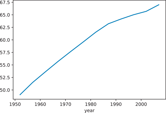
Figure 1.1 Basic plot in Pandas showing average life expectancy over time
Conclusion
This chapter explained how to load up a simple data set and start looking at specific observations. It may seem tedious at first to look at observations this way, especially if you are already familiar with the use of a spreadsheet program. Keep in mind that when doing data analytics, the goal is to produce reproducible results, not repeat repetitive tasks, and be able to combine multiple data sources as needed. Scripting languages give you that ability and flexibility.
Along the way, you learned about some of the fundamental programming abilities and data structures that Python has to offer. You also encountered a quick way to obtain aggregated statistics and plots. The next chapter goes into more detail about the Pandas DataFrame and Series objects, as well as other ways you can subset and visualize your data.
As you work your way through this book, if there is a concept or data structure that is foreign to you, check the various appendices for more information. Many fundamental programming features of Python are covered in the appendices.