
OpenGL was designed to provide two things: a portable yet powerful 3D graphics API and a narrow interface portal between the high-level calls and the low-level hardware interface routines. Although we’re interested mostly in the first item, it’s the second one that’s driving a lot of our actions. For OpenGL to be wildly successful, there’s got to be a synergy among the software developers (you!), the hardware platforms (mostly the video card manufacturers), and the operating systems (Windows 95, Windows NT, OS/2, and the UNIX flavors).
The operating systems have provided us with OpenGL implementations that we can work with. OpenGL was designed so that the generic implementation that comes with the operating system could be easily superseded by drivers provided for specific video hardware. This is a key issue. After all, Windows 3.x didn’t really become the largest GUI operating system on the face of the planet simply because it was better than anything else. Hardly! It became that way (despite Microsoft’s considerable marketing efforts) because the platform that it ran well on—a 16 MHz Intel 80286 with 1M of memory and a VGA display screen—not only was the current standard but also ran adequately on that platform. Slapping a multitasking GUI on the front of an application program means that you can expect about a 50 percent degradation in performance. The greatest bottleneck is usually just waiting around for all the graphics commands of the GUI to be executed. This led to the rapid development of specialized hardware on video cards that would install their own video drivers to take advantage of their hardware to speed up graphics commands. The result was many, many different hardware interfaces as these so-called super-VGA, or SVGA, cards came out. This was a nightmare for applications developers, who either had to get each hardware card’s specifications and write a driver (for writing a DOS program, for example), or else programmed only for Windows and let the user install the driver provided for the particular video card.
It was quite a painful period for nascent Windows programs, since the hardware manufacturers didn’t really understand that if they sent out slow or buggy software drivers, it made their hardware nearly useless. What good is fast hardware if it’s misprogrammed by a buggy driver?
Fortunately OpenGL was designed to avoid these problems, through the combination of a well-defined API and a test suite. This enables the video hardware manufacturers to choose what hardware enhancements to implement and to have their software drivers tested through the standard OpenGL test suite. Since the low-level API that calls can come through is so small, there isn’t a lot of room to make mistakes in the interface code, and the test suite will catch the majority of implementation problems. With the hardware manufacturers writing their own optimized driver code and with a test suite to catch most of the bugs, OpenGL applications can be written with good assurance that they will work better than average on anything other than generic implementations.
What does this have to do with drawing primitives? You might be surprised to see how limited the number of primitives is that OpenGL supports. After all, ten seems like such a small number! Ten? Yes! One type of point, three types of lines, and six types of polygons: OpenGL contains the barest minimum for creating objects. It’s a very powerful graphics interface with built-in effects, such as hidden-surface removal, shading, lighting, and texture mapping, but it’s very limited in the things that you can draw. This is by design, since the objective of a limited set of drawing primitives is to provide as clean and concise an API as possible and, in effect, to get as many hardware graphics accelerators manufactured as possible.
The other things that you usually want after you get basic drawing functionality, the lighting, the texture mapping, and so on are even more difficult to do than primitive creation, but that’s provided by the OpenGL API. By limiting you to the ten primitives in the API, you’re forced to write your own or to use the ones in the auxiliary library. This allows the graphics pipeline to be optimized for speed at the expense of forcing you to write your own macros to construct the objects you want. Once you get over the shock of having to create your own circle-drawing routine, you’ll be thankful that you don’t have to write your own texture-mapping code as well.
OpenGL has three basic types of primitives: points, lines, and polygons. Let’s start with the simplest.
Despite its one point primitive, OpenGL gives you a great deal of control over how the point looks. You control the size of a point, and you control the antialiasing of the point. This gives you great control over how a point is displayed. The default rendering of a point is simply a pixel. However, you can control the size to make points any number of pixels in diameter, even fractional pixels. If antialiasing is enabled, you’re not going to get half a pixel displayed, but OpenGL will “blur” the point across the pixels, or antialias the pixel, which gives the point the perceived effect of being located fractionally.
As with any OpenGL commands to create an object to render, we must wrapper the commands between a call to glBegin() and glEnd(), with the single argument for glBegin() being one of the ten enum values for the primitive you’re creating. A single argument to glBegin() creates a set of points.
That argument, GL_POINTS, draws a point at each vertex, for as many vertices as are specified. For example, if we wanted to draw four points in a diamond pattern about the origin, we might have the following code:
glBegin( GL_POINTS )
    glVertex2f( 0.0f, 2.0f ); // note 2D form
    glVertex2f( 1.0f, 0.0f );
    glVertex2f( 0.0f,-2.0f );
    glVertex2f(-1.0f, 0.0f );
glEnd();
The pixels that get drawn on the screen depend on a number of factors. Normally the locations of a point are reduced to a single pixel on the screen. If antialiasing is turned on, you might get a group of pixels of varying intensity instead, with the sum of their location representing a single pixel located across a couple of pixel boundaries. If you change the default pixel size with the glPointSize() command, the pixels drawn will then correspond to that size. If antialiasing is also turned on, the edges of the point might be slightly “fuzzed,” as OpenGL attempts to represent a point that doesn’t fall exactly on pixel boundaries.
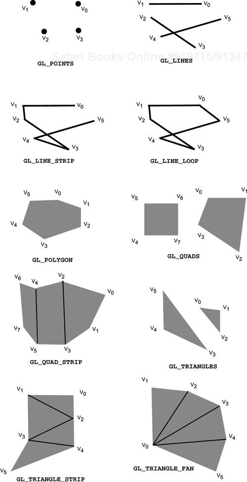
You can query the maximum and minimum sizes that your implementation allows for pixels by using the glGetFloatv() function with the GL_POINT_SIZE_RANGE argument. Check the OpenGL Reference Manual for the exact calling procedure. Figure 4.1 shows the entire collection of ten primitives that can be created in a call to glBegin().
OpenGL has a bit more latitude with the ability to manipulate lines. In addition to controlling line width, you can also specify stipple patterns. Lines are the first primitive we’ve seen that are really effected by lighting calculations. Unlike the points primitive, the order in which both lines and polygons have their vertexes given is important. When you construct your primitives, make sure that the order the vertexes are specified in is correct for the primitive you’re creating. Three different line primitives can be created:
GL_LINESdraws a line segment for each pair of vertices. Vertices v0 and v1 define the first line, v2 and v3 the next, and so on. If an odd number of vertices is given, the last one is ignored.GL_LINE_STRIPdraws a connected group of line segments from vertex v0 to vn, connecting a line between each vertex and the next in the order given.GL_LINE_LOOPdraws a connected group of line segments from vertex v0 to vn, connecting each vertex to the next with a line, in the order given, then closing the line by drawing a connecting line from vn to v0, defining a loop.
To draw the diamond pattern we used for the points, we’d just change the primitive specified in the glBegin() call. This will result in a parallelogram being draw.
glBegin( GL_LINE_LOOP )// make it a connected line segment
     glVertex2f( 0.0f, 2.0f ); // note 2D form
     glVertex2f( 1.0f, 0.0f );
     glVertex2f( 0.0f,-2.0f );
     glVertex2f(-1.0f, 0.0f );
glEnd();
Just as with points, the default size is one pixel, but you can control both the line size, using glLineWidth(), and the smoothness of the lines drawn with antialiasing. And again, just as with points, you can get the maximum and minimum line sizes by using the glGetFloatv() call with the appropriate arguments.
You can also specify patterned, or stippled, in the OpenGL vernacular, lines. These patterns are essentially a series of 0s and 1s specified in a 16-bit variable. For every 1 appearing in the pattern, drawing is turned on; a 0 turns drawing off. You can also increase the size of the pattern by specifying a multiplying factor. This allows you to make the patterns appear larger. When the full 16 bits have been used to draw with, the pattern is restarted. For example, a pattern of 0xFFFF renders a solid line, whereas 0xFF00 renders a dashed line, with the drawn and undrawn parts being of equal length.
If you are rendering a series of connected lines (that is, they are all in the same glBegin()/glEnd() sequence), the pattern continues across the connecting vertices. This is useful if you’re plotting data on a graph and want the pattern to continue along the entire length of the line or if you’re plotting a curved shape and want the pattern to flow along the curve, as the curve is really nothing more than a series of connected straight lines of very small intervals.
You can also control the width of stippled lines just as you would for solid lines. The width is independent of the pattern, so you have complete control over the line. If you need a line that contains a pattern in two or more colors, you can create patterns that draw only in the appropriate locations and then use those patterns to create multiple, overlapping lines. As long as you use the exact same vertices, you should get the effect you want, with only the occasional overlapping pixel being drawn in both colors; so use only opaque colors, and you’ll never notice.
Unlike the more comprehensive mathematical definition of a polygon, a polygon that OpenGL can render correctly is a simple, convex polygon of three or more unique points that all lie on the same plane. A polygon is simple if its edges don’t intersect; that is, two edges can’t cross without forming a vertex. A polygon is convex if it’s never dimpled inward—or mathematically speaking, that for any two vertices of the polygon, a line drawn between them remains on the interior of the polygon. By definition, the polygon must have three or more points; anything less is either a line or a point. Finally, all of the polygon’s points must lie on the same plane—any arbitrary plane, not just the three planes formed by intersections of the x-, y-, and z-axes. Figure 4.2 shows examples of simple and nonsimple polygons.
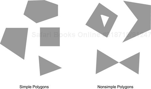
An example of a simple polygon with four vertices is a square of cloth with all four corners pinned to a tabletop. If you pull up one corner of the cloth, you have a curved surface—a nonsimple polygon.
OpenGL will be perfectly willing to attempt to render any nonsimple polygons; it’s up to you to make sure that you give it accurate information. There’ll be no warning if you enter a nonsimple polygon; what happens when you try to render one is undefined. Frequently OpenGL will do a creditable job of rendering polygons that are only slightly out of true; however, at certain angles the polygon will look inaccurate, and it’s agonizing trying to figure out what’s wrong. This is why triangles are so popular; with only three points, they have to lie on a plane. That’s why so many routines in OpenGL degenerate objects into groups of triangles, since triangles meet all the requirements of being simple, convex polygons.
Polygons are also the most fulfilling primitives, since they are the building blocks from which all the satisfying things are constructed. Polygons let you have a surface. A surface gives you the ability to specify fun things, such as color, opacity, the appearance of material it’s constructed from, and how light reflects off it. (Note that lines and points also share some of these attributes.) And these capabilities, combined, give you the ability to create realistic-looking objects.
You construct polygons just as you would a line segment. The following code constructs a filled-in parallelogram on the x-y plane.
glBegin( GL_POLYGON )
    glVertex2f( 0.0f, 0.0f ); // note 2D form
    glVertex2f( 1.0f, 1.0f );
    glVertex2f( 0.0f, 1.0f );
    glVertex2f( -1.0f, 0.0f );
glEnd();
Note that the order of the vertices is very important, since the order tells OpenGL which side of the polygon is the “front.” This is important when constructing enclosed objects or when only one side of an object will be visible. By judiciously constructing objects so that you need to render only the front faces, you can significantly increase performance at no expense to the rendering quality. The face of a polygon that’s rendered to the screen and that has a counterclockwise vertex order around the perimeter of the polygon is—by default—considered the front face of the polygon; a clockwise order denotes the back face.

By default both faces of a polygon are rendered. However, you can select which faces get drawn and how front faces are differentiated from back faces. This is another of those subtle points that can bite you if you aren’t paying attention. If you mix the order in which you draw your polygons, rendering becomes problematic, since you frequently don’t want the back-facing polygons to be displayed. For example, if you’re constructing an astounding 3D texture–mapped game in tribute to your favorite TV series, you probably don’t want the interior of the Romulan ships drawn. In fact, you probably don’t want OpenGL to bother with worrying about any of the faces of the objects that aren’t visible, so you specify that the back faces (or front faces if you like) can be ignored when rendering your scene, in order to boost performance.
How do you tell whether the polygon is going to be clockwise or counterclockwise in screen coordinates? After all, you can always move your viewpoint to the other side! Well, technically it’s complicated, but in practical terms just make sure that if the object has an “outside” or a “front,” that that side’s vertex order is counterclockwise.

You can control whether front-facing or back-facing polygons are rendered by the command glCullFace(), with a value indicating front or back faces. This will allow you to select which faces get culled. You toggle culling by using glEnable() with the appropriate arguments. You can swap the clockwise or counterclockwise designation of a “front” face by using the glFrontFace() command. Note that you can easily control the culling for an object by prefacing the modeling commands for it by the appropriate commands. Don’t forget to restore the attributes you’ll need later.
It’s also possible to individually control how the front and back faces are rendered. The glPolygonMode() command takes two parameters. The first parameter selects which side of the polygon we want to select: front facing, back facing, or both. The second parameter, the rendering mode, indicates that the polygon should be rendered as only vertex points, lines connecting the vertexes (a wire frame), or filled polygons. This is useful if your user may end up inside a model; you want to provide a hint that the user is inside. If the mode were filled polygons, the user would just see a screen full of color. If the mode were points (or back-face culling enabled), the user would probably see nothing recognizable. If the wire-frame mode were on, the user would probably quickly get the feeling of being inside the model. You can control which edges in a polygon are rendered and thus eliminate lines in the wire frame. This is discussed in the section on controlling polygon edge boundaries.
OpenGL can construct six types of polygon primitives, each optimized to assist in the construction of a particular type of surface. The following list describes the polygon types you can construct:
GL_POLYGONdraws a polygon from vertex v0 to vn–1. The value of n must be at least 3, and the vertices must specify a simple, convex polygon. These restrictions are not enforced by OpenGL. In other words, if you don’t specify the polygon according to the rules for the primitive, the results are undetermined. Unfortunately OpenGL will attempt to render an ill-defined polygon without notifying you, so you must construct all polygon primitives carefully.GL_QUADSdraws a series of separate four-sided polygons. The first quad is drawn using vertices v0, v1, v2, and v3. The next is drawn using v4, v5, v6, v7, and each following quad using the next four vertices specified. If n isn’t a multiple of 4, the extra vertices are ignored.GL_TRIANGLESdraws a series of separate three-sided polygons. The first triangle is drawn using vertices v0, v1, and v2. Each set of three vertices is used to draw a triangle.GL_QUAD_STRIPdraws a strip of connected quadrilaterals. The first quad is drawn using vertices v0, v1, v2, and v3. The next quad reuses the last two vertices (v2, v3) and uses the next two, in the order v5 and v4. Each of the following quads uses the last two vertices from the previous quad. In each case n must be at least 4 and a multiple of 2.GL_TRIANGLE_STRIPdraws a series of connected triangles. The first triangle is drawn using vertices v0, v1, and v2; the next uses v2, v1, and v3; the next v2, v3, and v4. Note that the order ensures that they all are oriented alike.GL_TRIANGLE_FANdraws a series of triangles connected about a common origin, vertex v0. The first triangle is drawn using vertices v0, v1, and v2; the next uses v0, v2, and v3; the next v0, v3, and v4.
As you can see, OpenGL is geared toward providing a rich, albeit limited set of primitives. Since this pipeline is so regulated, it provides a closed set of functionality for hardware manufacturers to implement. In other words they’ll be providing OpenGL hardware implementations that will be optimized in a standard way—in this case optimized rendering of just ten primitive types. As we’ll see later, having a hardware assist results in a huge improvement in speed.
In addition to stippling an OpenGL line, you can stipple a polygon. Instead of the default filled-polygon style, you can specify a pattern 32 bits by 32 bits that will be used to turn rendering off and on. The pattern is window aligned so that touching polygons using the same pattern will appear to continue the pattern. This also means that if polygons move and the viewpoint remains the same, the pattern will appear to be moving over the polygon!
The pattern can be placed in any consecutive 1024 bits, with a 4-by-32 GLubyte array being a convenient format. The storage format of the bytes can be controlled so that you can share bitmaps between machines that have different storage formats, but by default the storage format is the format of the particular machine your program is running on. The first byte is used to control drawing in the lower-left corner, with the bottom line being drawn first. Thus the last byte is used for the upper-right corner.
Suppose that you’d like to make a routine that draws a circle. It’s relatively easy to make a routine that draws a circle out of triangles—it’s just a matter of connecting a bunch of triangles that share a common center and have edge vertices spaced around the perimeter of the circle. However, although OpenGL handles the case of overlapping edges and vertices, with only one edge drawn even though two polygons share an edge, there is still an edge shared by two polygons. If the polygons are drawn as wire frames, both edges become visible. This might not be a problem if both polygon edges are the same color and are fully opaque. However, if they are translucent, the color of the shared edge will be calculated twice. Or, you might simply not want the underlying structure of a complex shape to be visible. In these cases you can turn edges on and off for each vertex by preceding that vertex (and any others that follow it) by prefacing the glVertex*() command with the glEdgeFlag*() command with the appropriate arguments. Using this argument, you can construct what appears to be a nonsimple polygon. The edge boundaries are automatically set for polygon strips and fans, so you can control the edge flag only for individual polygons you are constructing. Thus this command effects only the edges of individual triangles, individual quadrilaterals, and individual polygons, not any of the shared vertex primitives.
Since rectangles are frequently called in graphics applications, OpenGL contains a specialized call, glRect*(), that draws a rectangle. This call takes arguments that specify two opposing corner points and renders a rectangle on the x-y plane. You should note that glRect*() should not be called in a glBegin()/glEnd() sequence, since this command essentially encapsulates its own glBegin()/glEnd() pair. For example, the following line of code:
glRectf( 0.0f, 0.0f, 1.0f, 1.0f );
is precisely the same as the following sequence of commands:
glBegin( GL_QUADS );
    glVertex2f( 0.0f, 0.0f );
    glVertex2f( 1.0f, 0.0f );
    glVertex2f( 1.0f, 1.0f );
    glVertex2f( 0.0f, 1.0f );
glEnd();
The reason behind this command is, of course, speed. Rectangles render quickly, especially if the viewpoint is perpendicular, or nearly perpendicular, to the screen. So if you’re strictly interested in 2D rendering or in simple business graphics, you might get a big performance boost by using rectangles wherever possible.
Now that you’ve been exposed to the basic primitives, let’s go over what you need to do to try out some of them in your own code. In addition to specifying the type of primitive and the vertices that make up the primitive, you’ll need to specify colors for the vertices. If you’re interested in lighting for your model, you’ll also have to specify additional information with each vertex or polygon.
OpenGL is a state machine, and nowhere is it more obvious than in setting the color of a vertex. Unless explicitly changed, a state remains in effect. Once a color is selected, for example, all rendering will be done in that color. The glColor*() function is used to set the current rendering color. This family of functions takes three or four arguments: three RGB values and an (optional) alpha value. The glColor3f() function takes three floating-point values for the red, blue, and green color to select. A value of 0 means zero intensity; a value of 1.0 is full intensity, and any value in between is a partial intensity. Note that if you’re using a 256-color driver, you’ll probably get a dithered color.
Selecting a color is done for each vertex, but it’s also effected by the current shading model selected. If flat shading is currently selected, only one vertex is used to define the shaded color for the entire polygon. (Note that which vertex defines the shaded color depends on the primitive type. See the following section for more information.) If, however, we have smooth shading enabled (in OpenGL’s case, this means Gouraud shading), each vertex can have a unique shaded color (which depends on the vertex’s unshaded color—the color assigned that particular vertex and the current light falling on the vertex). What happens between vertices of different shaded colors is that the intermediate pixel’s colors are interpolated between the shaded colors of the vertices. Thus OpenGL will smoothly blend from the shaded color at one vertex to the shaded color of other vertices, all with no intervention from us. You can see the effects of lighting by examining Color Plate 9-1.
A normal vector is a vector that is perpendicular to a line or a polygon. A normal vector is shown in relationship to a polygon in Figure 4.3. Normal vectors are used to calculate the amount of light that’s hitting the surface of the polygon. If the normal vector is pointing directly at the light source, the full value of the light is hitting the surface. As the angle between the light source and the normal vector increases, the amount of light striking the surface decreases. Normals are usually defined along with the vertices of a model. You’ll need to define the normals of a surface if you’re going to use one of the lighting models that OpenGL provides.

You’ll need to define a normal for each vertex of each polygon that you’ll want to show the effects of incident lighting. The rendered color of each vertex is the color specified for that vertex, if lighting is disabled. If lighting is enabled, the rendered color of each vertex is computed from the specified color and the effects of lighting on that color. If you use the smooth-shading model, the colors across the surface of the polygon are interpolated from each of the vertices of the polygon. If flat shading is selected, only one normal from a specific vertex is used. If all you’re going to use is flat shading, you can significantly speed up your rendering time by not only selecting a faster shading model but also by not having to calculate any more than one normal for each polygon. For a single polygon the first vertex is used to specify the color. For all the other primitives it’s the last specified vertex in each polygon or line segment.
Calculating normals is relatively easy, especially if we’re restricted to simple polygons, as we are when using OpenGL primitives. Technically we can have a normal for either side of a polygon. But by convention normals specify the outside surface. Since we need at least three unique points to specify a planar surface, we can use three vertices of a simple polygon to calculate a normal. We take the three points and generate two vectors sharing a common origin. We then calculate the vector, or cross product, of these two vectors. The last step is to normalize the vector, which simply means making sure that the vector is a unit vector, meaning that it has a length of one unit. Listing 4.1 is some working code to calculate a unit normal vector. OpenGL will normalize all normal vectors for you, if you tell it to. But we can use this routine to provide only unit normals automatically. The following routine takes three vertices specified in counterclockwise order and calculates a unit normal vector based on those points.
Example 4.1. Code for Calculating a Unit Normal Vector
// Pass in three points, and a vector to be filled

void NormalVector( GLdouble p1[3], GLdouble p2[3],
                   GLdouble p3[3], GLdouble n[3] )
{
    GLdouble v1[3], v2[3], d;
    // calculate two vectors, using the middle point
    // as the common origin
    v1[0] = p2[0] - p1[0];
    v1[1] = p2[1] - p1[1];
    v1[2] = p2[2] - p1[2];
    v2[0] = p2[0] - p0[0];
    v2[1] = p2[1] - p0[1];
    v2[2] = p2[2] - p0[2];

    // calculate the cross-product of the two vectors
    n[0] = v1[1]*v2[2] - v2[1]*v1[2];
    n[1] = v1[2]*v2[0] - v2[2]*v1[0];
    n[2] = v1[0]*v2[1] - v2[0]*v1[1];

    // normalize the vector
    d = ( n[0]*n[0] + n[1]*n[1] + n[2]*n[2] );
    // try to catch very small vectors
    if ( d < (Gldouble)0.00000001)
        {
        // error, near zero length vector
        // do our best to recover
        d = (GLdouble)100000000.0;
        }
    else // take the square root
        {
        // multiplication is faster than division
        // so use reciprocal of the length
        d = (GLdouble)1.0/ sqrt( d );
        }
    n[0] *= d;
    n[1] *= d;
    n[2] *= d;
}
If you use this approach, you’ll get reasonably good results, with lighting effects that look good. However, you’ll get an artifact called faceting, which means that the shading on adjacent polygons is discontinuous, in some cases clearly showing the individual polygons that make up the surface. If this is unacceptable, you can switch to smooth shading. However, smooth shading, although interpolating between the vertices of a polygon, does nothing to make sure that the interpolygon shading is smooth. In this case you’ll need to either use a larger number of polygons to define your surface or modify the normals to simulate a smooth surface.
Analytic surfaces are defined by one or more equations. The easiest way of getting surface normals for such a surface is to be able to take the derivative of the equation(s). If the surface is being generated from a sampling function—one that provides interpolated values taken from a database—you’ll have to estimate the curvature of the surface and then get the normal from this estimate. Both of these approaches are beyond the scope of this book. An appendix in the OpenGL Programming Guide gives a very quick overview of what you’ll need to do if you’re interested in it.
An alternative is to take the information you’ve got and interpolate your own surface normals. To reduce faceting of all the vertices that are touching, you’ll need to make all those vertices have the same normal. The easiest way is to simply average all the normals of each vertex and to use this averaged value for all of them. For n polygons that share a common point, there are n vertices, and n individual normals. You need to add up all the normal values, n0 + n1 + n2 + ... + nn. Then normalize this vector and replace the original normal values with this one.
Another important item you’ll need to know is how to clear the rendering window. For simple 3D scene rendering, you’ll usually clear both the color buffer and the depth buffer. The color buffer is the current color of a pixel on the screen, whereas the depth buffer is the “distance” of that pixel from the viewpoint. See the discussion of the z-buffer in chapter 3. For now understand that we need to set the clear values for both the color and depth buffers, usually the color black for the color buffer and a value of 1.0 for the depth buffer. That’s done with the following commands:
glClearColor( 0.0f, 0.0f, 0.0f ); // set to black
glClearDepth( 1.0f );            // set to back of buffer
Once the clear color and clear depth values have been set, both buffers can be cleared with the following call:
// clear both buffers simultaneously
glClear( GL_COLOR_BUFFER_BIT | GL_DEPTH_BUFFER_BIT );
This command is usually issued just before you begin to render a scene, usually as the first rendering step in your response to a WM_PAINT message.
Creating primitives is the heart of 3D programming. It doesn’t matter if it’s a car widget or a Velociraptor; the really interesting things usually consist of one complicated thing made up of less complicated parts, made up of still simpler parts. Once you get a feel for creating your own primitives that you can file away for later reuse, you’re well on your way to creating your own “toolbox” of primitives that you’ll be able to reuse in a number of ways.
Of course, it’s not just creating primitives that make up those spectacular scenes from movies and flight simulators that you’ve seen. OpenGL still has some tricks to divulge about display lists (essentially an interpreted, replayable string of drawing commands) and texture mapping. Texture mapping is the ability to make a cube look like a five-story building, down to doors, windows, and bricks, with almost no extra effort (and almost no time penalty)! But that’s a subject for a later chapter. You should have a good idea about how to go about designing your own primitives. Start small and work your way up. Pick an object that’s pretty complicated and break it down into parts that you can model. Once you have all the parts, it’s a simple matter to put them together to form something spectacular!