Drainage calculations
Contributed by
E.D.Stewart, MA, PhD,
E.1
Theory
E.1.1
General mathematical model
The flow of water in the watertable of homogeneous isotropic soil is governed by Darcy's law:
where v is the effective velocity of water flow, K is the constant hydraulic conductivity, h is the hydraulic head.
The hydraulic head at any given point is
where z is the gravitational head, i.e. the vertical height above the origin of coordinates, and p is the pressure head.
In this appendix only steady flows will be considered, i.e. flows where the watertable is in equilibrium, with rainfall balancing drainage. For steady flows, conservation of water implies that inside the watertable
and so, from equation (E. 1)
The boundary conditions for this equation are:
1. for an impermeable boundary
where n is the unit outward-pointing vector perpendicular to the boundary of the water-table;
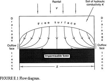
2. for an outflow face (Figure E. 1)
3. for a free surface with rainfall V
and
where żis the unit vertically upward-pointing vector and so –V ż is the effective velocity of rainfall flow.
Using equations (E.1) and (E.2) these become, in terms of h:
1.
2.
3.
E.1.2
Applying the general mathematical model to the case of two-dimensional flow on a horizontal, impermeable base, bounded by two drainage trenches, with rainfall V
From Figure E.l, the flow is clearly symmetrical so consider the right-hand side only (Figure E.2). This is a difficult problem to solve exactly
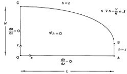
FIGURE E.2 Boundary conditions for differential equation.
but by using the following trick a bound can be obtained for H.
In the interior of the region OABC,=V20 and=V20 is an identity. Therefore
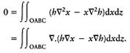
Now using the divergence theorem this is equal to an integral over the boundary of the region OABC:
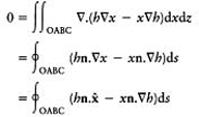
where is the unit vector (1,0).
Now using the boundary conditions (Figure E.2)
But
Therefore,
and since the watertable is in equilibrium with rainfall balancing drainage
where v=(ν x, v z) and so, from (E. 1),
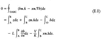
Thus, from (E.8)
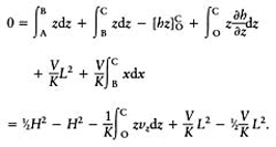
Therefore,
But on OC, ν z ≤0 and at O, ν z =0 and at C, ν z =–V. Also, on OC, ∂v x /∂x≥0 and so, from equation (E.3) ∂νz /∂z≤0. Thus
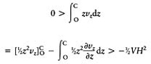
and so, from equation (E.9)
and so
or equivalently
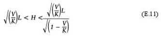
Now if K.V or L2 . H 2 (which are true for most practical cases) then a definite formula can be given:
E.1.3
Approximate method that will be used for practical calculations
For this method it is assumed that
i.e. the flow is approximately horizontal.
Now from equation (E. 1) condition (E. 14) is equivalent to
But from (E.7), h=z is one of the boundary conditions for the free surface of the water-table, therefore h(x,y) now gives the height of the free surface of the watertable.
Also, since the flow is steady with rainfall V, conservation of water now gives
where u is the depth of the watertable and v = (v x, v ) and so from (E.1)
The only sensible boundary condition is to set u
=0 where the soil meets a drainage trench. For two-dimensional flow this reduces to
Therefore,
with u=0 at a drainage trench boundary and where x=x 1 is the point where there is no flow of water. Now for the case discussed in section E. 1.2, u=h and x 1 =0. Therefore,
so that
where h=H at x=0 has been used.
Therefore
which is the equation of an ellipse.
Now setting u=0 at x=L, i.e. h=0 at x=L
which agrees with the result obtained in section E.1.2 in the limit L2 . H 2, i.e. for an approximately horizontal flow.
E.2
Practical calculations
E.2.1
Three-dimensional flow on a horizontal rectangular impermeable base bounded by drainage trenches with rainfall V
The watertable (Figure E.3) is determined from equation (E.15)
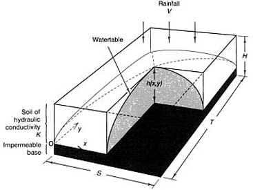
with u=0 on the boundary. The impermeable base is horizontal, therefore u=h. Let
Then equation (E.18) gives
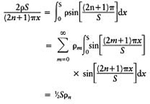
Expanding in Fourier series,
Now
Now equations (E.20)—(E.22) give
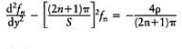
which has the general solution
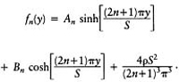
The boundary condition (E.20) now gives
Therefore
and
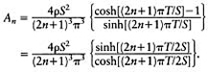
At peak capacity h(1/2S, 1/2T )=H, therefore
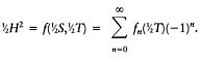
Now
and
Therefore,
Note that as T→∞ the problem reduces to the two-dimensional problem and we recover the two-dimensional result (E. 17), noting that S= 2L:
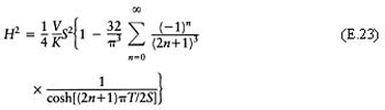
For T≥S the series (E.23) converges very quickly and can be very well approximated by
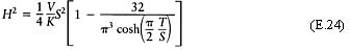
Of particular interest is the case of a square, T =S, when we get the formula
E.2.2
Two-dimensional flow on an impermeable base with constant slope G/S bounded by drainage trenches with rainfall V
The situation is represented by Figure E.4. The watertable is determined from equation (E.16)
with u=0 on the boundary.
The left-hand side of this equation gives the flow of water in the negative x direction at any given point as given by Darcy's law, while the right-hand side gives the flow of water needed to maintain equilibrium. The impermeable base has constant slope G/S and so
x=x 1 is the point where there is no flow of water. Let x=x 0 be the point where the watertable touches the surface of the soil, i.e.
Now from equations (E.26) and (E.27)
therefore
Also, from equations (E.26) and (E.27)
Let
and
and
Therefore,
Let
therefore
and
There are two cases:
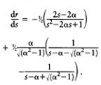
1. Case for a<l:
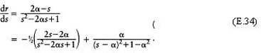
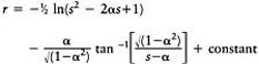
using the substitution s–α=√(l–α2) cot θ, equation (E.34) gives
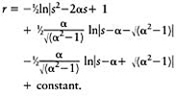
Therefore, from equation (E.33)
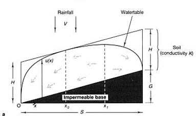
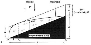
FIGURE E.4 (a) Two-dimensional flow on a constant slope with α>l. (b) Two-dimensional flow on a constant slope, with α<l.
Now the boundary condition (E.26) gives u =0 when x=0. Therefore, from equation (E.30), w=0 when t=1, and constant = 0.
Also, from equations (E.28)-(E.32)
when
Therefore, from equation (E.35) with constant=0,
Therefore
Also the boundary condition E.26 gives u= 0 when x=S. Therefore from equation (E. 30)
and from equation (E.35) with constant=0
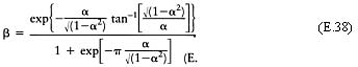
where tan- 1 (0 -)=π must be taken for a consistent definition of tan-1. Therefore
and from equation (E.36)
Now equations (E.29), (E.31) and (E.32) give
Therefore,
2. Case for a >1: from equation (E.34)
Therefore,
Therefore, from equation (E.33),
Now the boundary condition (E.26) gives u =0 when x=0. Therefore, from equation (E.30), w=0 when t=1.
Therefore
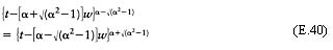
Now u=0 when x=0 or x=S and when u=0, i.e. w=0, equation (E.40) gives t= 0 or t=1. Therefore, from equation (E.30),
Now from equations (E.28)—(E.32) w=β when t=2αβ.
Therefore, from equation (E.40)
giving
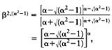
Now equations (E.29), (E.31), (E.32) and (EM) give
Therefore,
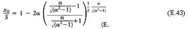
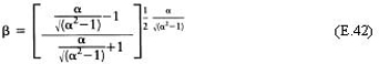
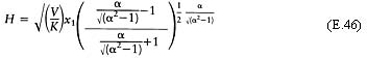
In summary, to calculate H or G use
and the graph of Figure 13.3(a).
To calculate S, K or V draw the straight line
on the graph and the point of intersection will give α and β, and hence from
will give S, K or V. The graph is given by equations (E.38) for α<l and (E.42) for α>l.
E.2.3
Two-dimensional flow on an impermeable base with optimum crowned profile bounded by drainage trenches with rainfall V
The situation is represented by Figure E.5. The profile is determined from equation (E.3)
For x<x 0 the situation is the same as in section E.2.2. From equations (E.31)-(E.32)
Now for α<l, equations (E.31), (E.32) and (E.36) give
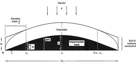
FIGURE E.5 Two-dimensional flow on a crowned profile.
and for α<l, equations (E.31), (E.32), (E.41)and (E.42) give (E.42)
Now equation (E.29) gives
For x 0<x<2x 1-x 0, u=H and h=g+H and so, from equation (E.44)
Therefore
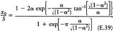
Now, when x=x 0, g=(G/S) x 0. Therefore, from equations (E.47) and (E.48)
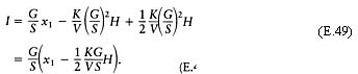
Therefore
where H is given by equations (E.45) and (E.46).
In summary, to calculate H, xl or G/S use equation (E.31)
and
together with the graph of Figure 13.3 (b).
To calculate K or V draw the straight line
on the graph and the point of intersection will give a and , and hence from
The graph is given by equations (E.45) for α<1 and (E.46) for α>l.
The profile is given by
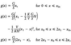
and