
Chapter 3
The Cycle of Data
Introduction
One of the most significant challenges to succeeding with augmented intelligence is the need to consistently manage data so that it can be applied to critical business problems. Many companies make the mistake of selecting a data source without doing the hard work of getting the data ready for use. There is a cycle of managing data that begins with data acquisition, moves on to data preparation, and progresses to the building of a predictive model based on the data. Data is needed to build and test the predictive models that are core to augmented intelligence. The work then cycles back to data acquisition in support of model improvement and ongoing model maintenance.
As we discussed in Chapter 2, we have made the movement from the traditional database model to a big data focus driven by the revolutions happening in infrastructure. The transition from traditional analytics to augmented intelligence requires a foundation of big data as part of the journey. You can’t simply move from a traditional packaged application and a relational database to augmented intelligence.
Traditional business applications and data management practices cannot support augmented intelligence. What are the traditional business applications currently in use in most organizations? These applications fall into two broad categories: transactional applications, which capture operational data such as customer orders or claims, and reporting applications that keep track of how well a business performed in the past, such as sales by product line and profit and loss. By contrast, augmented intelligence relies on predictive analytics intended to discover patterns in historical data so that this data can be used to predict the future.
How are predictive applications different from traditional business applications? The most important aspect of a predictive application is that it provides a technique to guide decision making. Predicting future events is much more complex than simply reporting on what has already taken place. The only way to truly begin to understand where your business is headed is to leverage a vast array of data from both inside and outside of the company. The analysis of such a rich data set via machine intelligence enables the data scientist to discover patterns in earlier business events that enable them to predict future outcomes. This knowledge provides guidance on the course of action the data scientist should take that will likely yield the best result. An action can be generated automatically by the machine learning algorithm if the process itself is straightforward. On the other hand, complex decision making will require that the machine learning process provide guidance to decision makers.
The use of machine learning algorithms for predictive analytics is powerful and can be used for both collaboration and knowledge transfer and personalization. The bottom line is that there are multiple techniques for leveraging machine learning to enhance the ability for businesses to solve complex problems. What is the difference between a collaborative approach and personalization?
Knowledge Transfer
Knowledge transfer across an organization is essential to the success of every organization. Knowing how the best performers use data to get work done is especially valuable. Such knowledge can make a junior employee more productive. For example, an experienced sales representative knows when to continue to nurture a lead and when to move on, based on a customer’s response to actions taken in the sales process. Providing predictive model-guided recommendations to a junior sales representative on the next best action to take in pursuing a lead is an effective means of knowledge transfer.
Personalization
Machine intelligence allows businesses to deliver a personalized experience to customers, employees, and suppliers. This personalization is based on an analysis of data on each person’s communication style and preferences. The success of a personalized communication strategy depends on the development of compelling content and the delivery of the content at the right time to the right individual. Businesses use models that predict likely customer response to identify what content to deliver to each customer and when the delivery should take place.
Determining the Right Data for Building Models
Simply put, you must have the appropriate data and the right amount of data to build predictive models. But as we mentioned in Chapter 2, it is not enough to simply apply data to creating a model. You have to begin by establishing the “training data set.” In many cases, the most common type of machine learning is supervised learning. The training data provides examples of input data (the independent variables) and output data (the dependent or target variable). Supervised learning seeks to infer a function between the input variables and the target variable we seek to predict. The resulting function or model is then tested on new data (called the “test data set”). The test data has the same structure as the training data, containing the same input features and the target feature (the correct answer). The accuracy of the function in predicting the target feature is evaluated. Several iterations of training, building, and testing follow.
The success of the model-building process depends on the quality, breadth, and relevance of the data used to train and test the model. Consider, for example, a data set related to real estate. There are records for each property that contain features about the property. These features include the property identifier, lot size, house size, number of rooms, location, and taxes billed. There are also related records of sales transactions for properties. The sales transaction records contain the property identifier as a link to the property records, along with features for buyer, seller, mortgage supplier, transaction date, and selling price. The property records and sales transaction records are merged using the property identifier feature that is common to both sets of records.
The merged data set (real estate data) is the source of candidate features for the development of a model to predict the current market value of the property. For a model to predict real estate prices, features in the real estate data set such as lot size, interior space in the house, number of rooms, and location are potential input features for the function expressed by the model. The target feature is the actual sales price, as recorded in the property sales transaction records.
The Phases of the Data Cycle
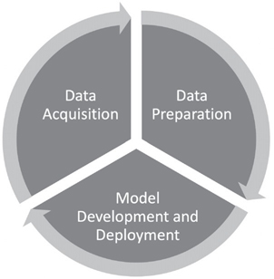
Figure 3-1 illustrates the three phases of the data cycle in support of the development of a predictive model which includes acquiring the data, preparing the data, and using the data to build the predictive model.
The three phases of the data cycle form an iterative feedback loop:
-
Data acquisition: Some of the data needed for model building may already exist within an organization. Other data to supplement the internal data can be acquired. This data may include product lists, order transactions, and equipment maintenance records. Unstructured data such as best practice documents, history, and regulations are also important for context and understanding. Data management specialists within the IT or corporate data function load data sets into a shared resource to be drawn upon for a range of modeling projects across business groups. Line of business (LOB) data scientists and business analysts may seek to acquire supplementary data, as needed, for specific modeling projects. Before the supplementary data may be used, permissions must be obtained from data owners.
-
Data preparation: Data scientists and LOB analysts explore relevant data sets and their relationships to one another. The exploration uncovers errors and anomalies that must be addressed in a process known as data cleansing. Then the features or attributes of the data are examined for the purpose of selecting the input variables with the best chance of predicting the target feature. Features are added or subtracted to aid in the development of the model. This step is called “feature engineering.”
-
Model development and deployment: With the help of domain experts, data scientists build and test predictive models using statistical and machine learning techniques. Based on the preliminary testing results, feature engineering may resume in an effort to improve the model’s capability to generate accurate predictions of the target variable. When testing shows that the model has achieved an acceptable level of accuracy, the model is ready for deployment. While in use, the model’s operational performance and accuracy continues to be monitored.
-
Back to acquisition: Based on ongoing testing and evaluation of the model, additional data may be needed in order to improve the accuracy of the model’s predictions. This need for additional data triggers a new round of data acquisition. Thus, the data cycle continues: returning to data acquisition, followed by data preparation, then to model maintenance and redevelopment.
Each of these aspects of the data cycle is complex and requires explanation. In this next section, we will delve into each aspect of the cycle and explore the nuances required.
Data Acquisition
To build a new predictive model, a business needs good data. To gain competitive advantage, a business must leverage the data it already possesses and acquire supplementary data, as needed, for model development. To be successful, it is mandatory to understand the details of all of your existing data, including its origin and usage. It is also critical to understand what information is missing. Once your organization collects all of the data required, you are ready to prepare your data for building models.
Identifying Data Already within the Organization
Businesses capture data about their products and customers during ongoing operations. Yet in some cases, teams may not realize that the organization already possesses a tremendous amount of data and knowledge. Often a business’s organizational structure may work against the ability and willingness of groups to share data. One of the consequences of this isolation is that decisions can be made without the proper context. Smart business leaders understand the value of learning from data across the company.
Consider the following situation at an international cruise line. Marketing operations within the cruise line were divided between two groups. One group was responsible for marketing the daily excursions offered during a cruise, while another group was responsible for marketing the cruises themselves. The marketing team responsible for promoting excursions during a cruise was proud of a new program for marketing daily excursions to customers while they were on a cruise.
Here is how the program worked. Each day, every customer received a personalized communication in the form of a custom newsletter left under the door of his or her cabin describing the excursions available that day. The featured excursions took account of individual cruisegoer preferences identified by the predictive model. The delivery of personalized communications to cruise passengers on the day excursions were offered resulted in a significant increase in daily sales.
That was an excellent outcome for the cruise line. But this data on customer preferences for activities during a cruise was valuable for other marketing activities as well. Specifically, information about the excursions a customer preferred would also help marketers identify which future cruise the customer might enjoy. The marketing team could then target potential customers for cruises that featured the types of activities they had selected for daily excursions. Yet the data on excursion preferences during a cruise was not part of the customer data sets used by the group responsible for marketing the cruises. Additionally, correspondence and reviews of excursions could also help to ensure that marketers understood what changes could improve their offerings. Eventually, management recognized that combining the customer excursion and customer cruise data could result in increased revenue across both organizations.
Once management mandated that the two organizations should collaborate, the two data sets were combined. The resulting merged data sets yielded better insights on customer preferences, both for cruises and for cruise excursions. Each group improved its marketing outcomes by leveraging the expanded, enriched data. The new information on customer preferences was shared with travel professionals so that they could offer customers new cruise packages that helped to drive additional incremental revenue.
Reasons for Acquiring Additional Data
Sometimes, not all of the required data is currently available within the organization. In that case, the company may need to collect additional data. For example, industrial companies with big capital investments in heavy equipment are investing in the development of models that predict when the equipment is likely to fail. With the predictions, a company can intervene to repair the equipment before it fails. But before the models can be built, new sensors must be installed on the equipment to acquire data on the performance of the equipment. Analysis of the sensor data integrated with other data about the equipment previously acquired enables the discovery of patterns that predict either continued normal operations or the likelihood of specific types of equipment failure. The prediction of a type of imminent failure leads to a recommendation of the specific repair needed to avert the failure.
In other situations, organizations may need to collect data aggregated from outside sources. When a model’s training data is limited to data captured within the organization, there is a risk of perpetuating an organization’s biases. Therefore, external data may help avoid unintended biases. For example, if a data scientist builds a candidate-selection model based solely on data regarding the performance of current employees, the model is likely to be biased. Training a model based on attributes similar to the successful employees may result in discriminatory hiring practices by missing good candidates who are different from those already in the organization. Discriminatory hiring practices can dramatically hurt a company’s reputation and can result in legal liability. A more broad set that includes outside data can address such problems. Professional associations, Internet employment sites, or government agencies have data on the attributes of people in particular occupations across an industry or across multiple firms. These sources can provide data on candidates with attributes different from the company’s current employees.
Consider the demographics of a major symphony orchestra from 50 years ago. White male hiring managers employed musicians who were like them. It was uncommon for women or people of color to be hired. How has this practice evolved? Many orchestras introduced blind auditions into the hiring process. The revised process required hiring managers to judge candidates who auditioned from behind a curtain. Judges had no knowledge of the gender or race of the candidate while they listened to his or her musical performance. This single process modification resulted in a far more varied population of musicians, and, arguably, a higher quality of overall orchestra performance. Data collected on employees across symphony orchestras today would yield a far more diverse data set. Predictive models trained on this data would not be limited by the biased hiring policies of the past.
These examples show that it’s not the sheer quantity of data that makes for the best training data set. A data set, even if quite large, may be homogeneous and incorporate the same limitations. Protecting the model from inherent bias depends on the richness and diversity of the data. Data variety can be more important than data volume for successful training of a predictive model.
Data Preparation
Once the data is acquired, it must be prepared. Data preparation requires an organizational commitment to the ongoing management of the data cycle that includes all of the key constituents, including data professionals, LOB application specialists, subject matter experts, and business analysts. Preparation improves the quality of the data used to train predictive models. Analytics and model building are actually only about 20% of the effort. Data preparation is where as much as 80% of the work is accomplished. Good data preparation is very challenging for the following reasons:
-
Labor intensive: There are many data tasks that are extremely labor intensive. In some cases, employees are required to input the same data into multiple applications. This leads to errors, wasted time, and added costs. Automation based on machine learning models is beginning to be used to reduce these errors and costs.
-
Relevance and context: It are common for an organization to collect data sources that seem logical, only to discover that the context is not correct. Sometimes the data source that seems relevant may be out of date. In other situations, the data source may include sensitive data that cannot be shared.
-
Complexity: It used to be the case that analytics and model buildings were based entirely on structured data. This data is typically predefined and, therefore, simpler to access. But with the advent of big data, organizations need to be able to leverage multiple types of data. Data may be in the form of images, text, or sound, where the structure has not been predefined. This type of data requires preprocessing to learn its actual structure so that the data can be analyzed in context. For example, later in this chapter, a case study shows how an online travel aggregator derives additional features about locations (hotels, restaurants, tours, etc.) by analyzing the language in user reviews. This new information then can be blended in with data about these same entities found in the structured data sources to yield an enriched data set.
-
Anomalies: Separate data sets may contain data on the same suppliers or customers. But the suppliers or customers may be referred to by different names or have different identifiers. These anomalies must be resolved before data on entities from separately maintained sources can be merged. There can also be missing values for specific data features that must be resolved in a consistent way across the data sources.
Data preparation has traditionally been the domain of data management professionals. However, it is equally important to include business analysts who have specific domain knowledge to evaluate data sources for potential use in their LOB. Today, new self-service methods of data cleansing are available for use by LOB specialists to participate in the data preparation process. The following case study of data preparation used a self-service (“data wrangling”) approach to address data anomalies. A key issue to resolve was missing data on defendants and co-defendants, which made it difficult to meet a court mandate to identify people who were convicted based on falsified drug tests. This issue of falsified drug tests is discussed in more detail in the box on the next page.
Preparing Data for Machine Learning and AI
One of the most important issues in the cycle of data is to make sure that you have selected the right data sources that are prepared in the correct manner that produces the right results. One of the greatest dangers is that an analyst grabs data sources that are inaccurate. The consequences can be dire if your organization is using the analytics to predict which direction to take your products and services. So, how do you make sure that you are preparing your data to support advanced machine learning and artificial intelligence (AI). There are three major steps in data preparation:
-
Data exploration
-
Data cleansing
-
Feature engineering
Data Exploration
Before beginning data preparation, it is imperative to gain an understanding of the data. To get started, it is imperative to be able to explore the data that seems to be pertinent to the problem your organization is trying to solve. Data scientists and business analysts need to become familiar with the features of the data. This exploration will reveal the relationships among the data sets so they can potentially be merged. Analysts also need to gain insights into the correctness of the data. There may be errors and anomalies that will impact results. This exploration will identify which features appear to have the greatest impact on the dependent variable—the result that the model seeks to predict.
Data exploration seeks to answer the following questions:
-
What are the available features within the data?
-
Is the data complete, or are there a lot of missing values?
-
Are there features that are correlated with each other?
-
What is the correlation of individual features with the target variable?
Data Cleansing
Once errors and anomalies in the data have been identified in data exploration, they can be managed through a process known as data cleansing. This phase seeks to remediate the errors and anomalies that have been discovered. Data cleansing requires strategies for the handling of missing values and resolving inconsistencies in data features to identify entities. These identifiers are required to link separate data sets together on the same subject. The work can be partially automated via machine learning algorithms that use pattern- matching techniques. However, subject matter experts must be involved to ensure that the correct data is being ingested into the model.
To understand the relationship between data exploration and data cleansing, consider the issues of missing values and inconsistent values. These anomalies are discovered in data exploration and addressed in data cleansing:
-
Missing values: Some records may be missing values for various features or fields. A quick fix for missing values in a field is to average out all of the present values in a data set for a field and then rely on this average or mean value to replace each missing value for that feature. But this method is overly simplistic and may not yield the best results. Machine learning algorithms can examine patterns in the other fields of a record in order to derive a better estimate. For example, if the value of the total interior size of a house is missing, data on the number of rooms can be used to derive a better estimate. An even better estimate might combine data on the number of rooms with data on the age of the house—since room size tends to vary depending on when the house was built. Location data (such as zip code/postal code) can also be factored in, as homes in certain geographic areas tend to have larger rooms than homes in other areas.
-
Inconsistent values: There may be inconsistent values for fields, which prevents the merging of data from multiple sources about a single entity. For example, the same company may have different names across data sets, or even within the same data set. For example, “IBM,” “International Business Machines,” and “IBM, Inc.” all refer to the same entity. Machine learning algorithms can detect inconsistencies in the data and then address the problem by mapping the different names to a single entity name. Human domain specialists then can review this work and flag false matches. The algorithm learns from this feedback and applies a modified strategy on the next round. Over time, the matching algorithm improves, resulting in a reduced percentage of false matches.
To see how data exploration and data cleansing operate together in practice, we’ll examine the data preparation strategies used by entrants in the Zillow competition to build a model to predict housing prices. Zillow, the popular real estate site, recently conducted an open contest for improving their Z-estimate model that assigns a market value to 110 million homes in the United States. The individual data science competitors were provided a real estate data set on the Kaggle website (a platform established as a platform for competitions among data science teams).4 The data had been merged from the multiple sources that Zillow uses for its Zestimate model. Zillow described the sources of the data it uses for calculating its Zestimates:
To calculate the Zestimate home valuation, Zillow uses data from county and tax assessor records, and direct feeds from hundreds of multiple listing services and brokerages. Additionally, homeowners have the ability to update facts about their homes, which may result in a change to their Zestimate.5,6
Contestants were then tasked with predicting the log of the error between the Z-estimate value and the actual sale price for the property. Zillow claimed that prior to the competition their Z-estimate had improved to within 5% of the actual price.
Several entrants in the Zillow competition documented how they explored the data provided on the Kaggle site and the strategies they used to deal with the anomalies they found. The first challenge they faced was the 56 features in the property data set. That’s an unwieldy number of features to evaluate as candidate predictors of property value.
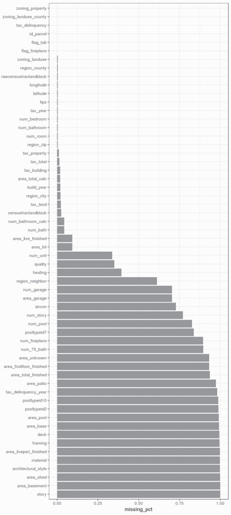
The second major challenge was the large percentage of missing values, which impacted data quality. Figure 3-2 shows a visualization of the features in the Zillow/Kaggle data set with the highest percentage of missing values. The features are ordered in ascending order according to percentage of missing values.
Based on what you’ve learned about the data set, you may decide to delete the features with the greatest percentage of missing values—for example, those with >75% missing value. Alternatively, you could look to estimate values that are missing when there is a high correlation between two variables.
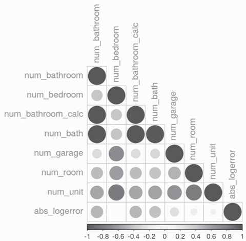
For example, further data exploration reveals that the bedroom-count feature turns out to be highly correlated with the bathroom-count feature. That makes sense, since a house with fewer bedrooms would logically require fewer bathrooms. You could develop a function to express the relationship between the two features. Using this approach, you could calculate the value of the of the feature with the missing value based on the feature where the value is present. You could also create a new feature—total-room-count—adding the values of bedroom-count and bathroom-count together. Figure 3-3 shows the correlation between different features. The larger and darker circles indicate a stronger correlation.
Deciding on which features to keep, which to delete, and which to create is the process of feature engineering. Here is where you apply the learning gained in data exploration in order to upgrade the quality of the data available for predictive model development.
Feature Engineering
Feature engineering is the refining of the features on the data set for use in predictive model development via a process of feature selection and feature creation. Feature engineering is an art that requires domain knowledge, data skills, and creativity to be performed effectively.
There are several approaches to feature engineering in which you prepare the data set for predictive model development.
-
Feature selection: You decide which features to delete and which to retain in a data set, applying the learning from data exploration and your knowledge about the domain of the prediction you are trying to build. For example, as noted in the last section, you could decide to delete those features with a high percentage of missing values, only retaining those features with a low percentage of missing values.
-
Feature creation: You can derive new features out of the existing data via various methods of calculation, binning, or extraction.
-
Feature creation via calculation: For example, we noted in the last section that a new feature—total-room-count—could be derived by adding together the values for the count of bedrooms and the count of bathrooms. The new feature had fewer missing values than either of the two original features. Another example is zip code and Federal Information Processing Standard (FIPS) code, both indicators of geographic location. Combining these two features into a new feature could reduce the percentage of missing values as compared to either feature alone.
-
Feature creation via binning: Classifying feature values into a category use a technique known as statistical data binning (a way to group data about a specific like value). This is useful for numeric values in a continuous range. You could group people via their age into millennials, gen-Xers, or baby boomers by specifying a beginning and an ending birth date. This groups values from a date or number into a category with a limited set of possible values. Another form of binning is used in finance to group accounts in aging categories—accounts less than 30 days old, 30–60 days old, and so on.
-
-
Feature creation via binning for non-numeric data: Creating new features out of raw data is not only limited to numeric data. For example, you could classify movies according to type: action, romantic comedy, horror, and so on. Software that analyzes text can be applied to the movie review to extract a variety of classification features that denote movie type. Software that analyzes images can classify an image as cat or dog, happy or sad. For classification data, the value of the feature is binary (Y or N).
Overfitting versus Underfitting
Adding features to a data set increases the set of variables available as predictors. But adding too many features may increase the time required to train the model. And the resulting model, by aligning with every data point of the training set, may not project well to new data. Such a model follows the noise in a particular data set, but misses the pattern that holds across data sets. This is the problem of overfitting. The opposite problem of overfitting is underfitting. Underfitting occurs when a model of low complexity does not align well with the training data. The model may have been built on too few features to capture the underlying pattern in the data. For such an oversimplified model, there is a high degree of error between the value predicted by the model and the actual value in the training data.
This discussion points to two characteristics that can be used to describe predictive models. Bias is the degree to which a model oversimplifies the relationships inherent in the data. Variance is the degree to which a model follows a specific data set too closely. Overfitting is a condition wherein the model has low bias, but high variance. Underfitting is a condition wherein the model has high bias, but low variance. Models that exhibit either overfitting or underfitting are unlikely to generalize well, failing to predict values accurately when exposed to data sets outside of the training data set. The best models strike a balance between overfitting and underfitting, capturing the pattern and not the noise within the data.
Overfitting versus Underfitting for a Model Predicting Housing Prices
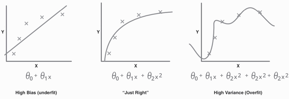
To better understand the challenges of overfitting and underfitting, it is helpful to compare the three charts in Figure 3-4. Each chart shows the same set of data points relating the price of a house (Y-axis) and the size of a house (X-axis). The model in each chart is the line drawn through the data points that expresses the relationship between house size and house price.
This chart depicts a simple model. It was built by a linear regression algorithm that yielded a straight-line function. This model assumes that as square footage goes up, price goes up in a linear fashion, that is, with a constant rate of change. A look at the chart shows that there are significant differences or errors between the model’s predicted values and the actual values in the data. It is not surprising that other factors (such as location) have a big impact in determining price. We know, for example, that a smaller house in a fancy neighborhood costs much more than a larger house in a run-down neighborhood. If that’s true, then the relationship between house price and house size cannot be linear. A model that relies on simplifying assumptions, missing the true relationship, is said to have high bias. The flaws in this model illustrate the problem of underfitting.
The chart on the right illustrates a model that expresses the relationship between square footage and price as a fourth-degree polynomial. This model fits the data points of the training data set the closest of the three alternatives shown. But it’s hard to believe that this model with its many ups and downs can generalize well to new data. New data (not part of the training data set) would almost surely not have this detailed pattern of sudden price increases and price decreases at precisely these size points. This model is said to have high variance, with too much dependence on the details of the test data set. Variance refers to the amount by which a model would change if we trained it on a different data set. The flaws in this model illustrate the problem of overfitting.
The chart in the middle assumes that the relationship between square footage and price is a smooth curve that can be expressed by a quadratic equation. This function looks to express the overall trend in the data the best of the three alternatives. This model is likely to perform better than the other alternatives when applied to new data, which is different than the training data. It sets the right balance between bias and variance—that is, between underfitting and overfitting.
In practice, overfitting is a far more common problem than underfitting. So how can you guard against overfitting? Here are several suggestions:
-
Reduce the number of features in the data set: Deleting features that are either redundant or unrelated to the outcome the model seeks to predict can reduce the risk of overfitting.
-
Expand the data set: Another corrective for overfitting is to increase the size of the data set. The portion for training and the portion for testing will each be larger. To be effective, this strategy requires that the expanded data set is not only bigger but also more diversified. Recall that hiring bias, not by superior performance, caused the overrepresentation of male musicians in symphony orchestras several decades ago. Expanding the training data with similar data from other orchestras of the time would not have helped.
-
Ensemble modeling techniques: An ensemble approach to machine learning, such as random forest, can be helpful in guarding against over-fitting. Random forest is a machine learning algorithm that creates multiple decision trees. The average prediction of the individual trees is selected to be the resulting model. Basing the final model on the results of multiple modeling efforts reduces the risk of a single modeling effort following the noise in the data. This ensemble approach to machine learning has been proven to be a method that can address the related issues of overfitting and accidental correlations.
From Model Development and Deployment Back to Data Acquisition and Preparation
With a prepared data set as the foundation, a predictive model is developed using a combination of features (the input variables) to predict the target feature (the output variable). For example, a real estate model to predict market prices relies on data about a house (features such as number and type of rooms, size, location, and age) in order to predict the target feature—selling price.
For a machine learning application, the data is typically split on a ratio of 90/10 between a training data set and a test data set. The training data set is used for learning which feature or combination of features have the greatest impact on the target feature—selling price—the feature which we seek to predict. The other portion of the data is held out as a test set used to evaluate how accurately the model predicts the actual sale prices at a point in time.
The data cycle continues after model development to data acquisition and data preparation. After initial model development, additional data preparation may be required. For example, the data scientist may need to create new features or delete some existing features. In many cases, more data may need to be added. A revised model is then developed and tested. The cycle continues until the model is ready for production.