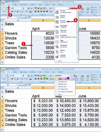
You can use number formatting to control the appearance of numerical data in your worksheet. For example, if you have a column of prices, you can apply currency formatting to the data to format the numbers with dollar signs and decimal points. Excel offers several different number categories, or styles, from which to choose.
Change Number Formats
Note
See Chapter 9 to learn how to select cells; see Chapter 11 to learn about ranges.
Note
You can apply number formatting to single cells, ranges, columns, rows, or an entire worksheet.
Excel applies the number formatting to the data.
Note
What sort of number formats can I apply to my numeric data?
Each number format style is designed for a specific use. The table below explains each number category:
Style | Style |
|---|---|
General | The default category; no specific formatting is applied |
Number | General number display with two default decimal places |
Currency | Adds dollar signs and decimals to display monetary values |
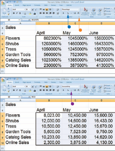
Accounting | Lines up currency symbols and decimal points in a column |
Short Date | Used to display short date strings |
Long Date | Used to display long date strings |
Time | Used to display time values |
Percentage | Multiplies cell value by 100 and displays percent sign |
Fraction | Displays value as a specified fraction |
Scientific | Uses scientific or exponential notation |
Text | Treats values as text |
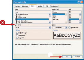
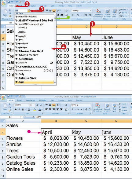
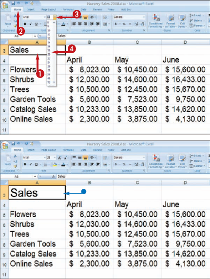
You can control the font that you use for your worksheet data, along with the size of the data text. For example, you may want to make the worksheet title larger than the rest of the data, or you may want to resize the font for the entire worksheet to a more legible size to make the data easier to read.

Change the Font and Size
CHANGE THE FONT
Note
See Chapter 9 to learn how to select cells.
You can also begin typing a font name to choose a font.
CHANGE THE FONT
Note
See Chapter 9 to learn how to select cells.
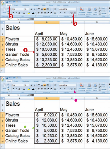
You can control the number of decimals that appear with numeric data using the Increase Decimal and Decrease Decimal commands. For example, you may want to increase the number of decimals shown in a cell, or reduce the number of decimals in a formula result.
Increase or Decrease Decimals

Note
See Chapter 9 to learn how to select cells; see Chapter 11 to learn about ranges. 3


You can click Increase Decimal (
You can click Decrease Decimal (
Excel adjusts the number of decimals that appear in the cell or cells.
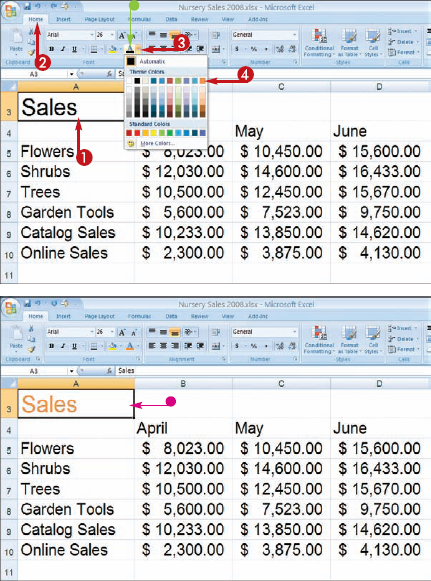
When adding color to worksheets, you You can change should always the color of your data, consider the color's Rent whether the data is numeric or effect on the Car text. For example, you might choose legibility of your Utilities a brighter color for any cell data to data, both in print Gasoline which you want to bring attention, and on-screen. You Food or select a different color for want your worksheet Total 1300 the column headers in to appear easy to your worksheet. read, not jarring and distracting to the eye.

You can change the color of your data, whether the data is numeric or text. For example, you might choose a brighter color for any cell data to which you want to bring attention, or select a different color for the column headers in your worksheet.
Change Data Color

Note
See Chapter 9 to learn how to 4 select cells; see Chapter 11 to learn about ranges.


You can control the alignment of data within your worksheet cells. By default, Excel automatically aligns text data to the left and number data to the right. Data is also aligned vertically to sit at the bottom of the cell. You can change horizontal and vertical alignments to improve the appearance of your worksheet data.
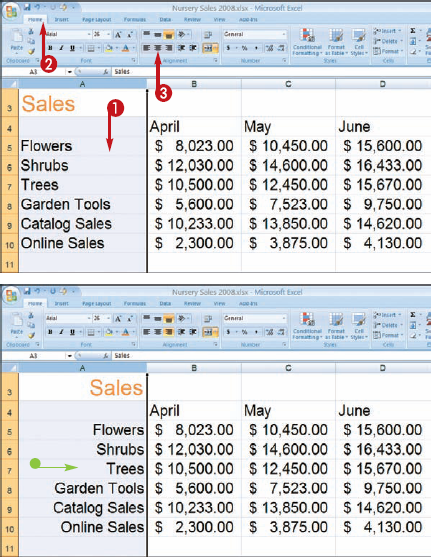
Adjust the Cell Alignment
SET HORIZONTAL ALIGNMENT

Note
See Chapter 9 to learn how to select cells.


Click the Align Left button (
Click the Center button (
Click the Align Right button (
Excel immediately applies the alignment to your cells.
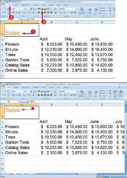
SET VERTICAL ALIGNMENT

Note
See Chapter 9 to learn how to select cells.


Click the Top Align button (
Click the Middle Align button (
Click the Bottom Align button (
Excel immediately applies the alignment to your cells.
Note
How do I set indents for my cell text?
You can use the Increase Indent and Decrease Indent buttons to add indents to lines of text in your worksheet. To indent text, click the Increase Indent button (

Can I justify my text to create left and right margins in a cell?
Yes. To justify cell text, you must open the Format Cells dialog box and display the Alignment tab. To do so, click the Font Dialog button (

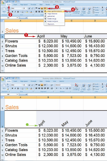
You can use Excel's Orientation command to rotate data in a cell. For example, you might angle column labels to make them easier to distinguish from one another. You can also angle the column labels to format data better on your printed spreadsheet.

Control Data Orientation

Note
See Chapter 9 to learn how to select cells.


Excel applies the orientation to the cell or cells.
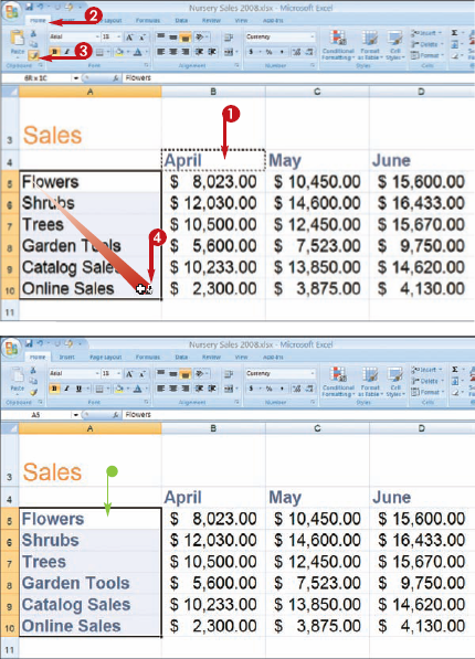
You can use the Format Painter feature to copy formatting to other cells in your worksheet. For example, you may have applied a variety of formatting options to a range of cells to create a certain look. When you want to re-create the same look elsewhere in the worksheet, you do not have to repeat the same steps that you applied to assign the original formatting. Instead, you can paint the formatting to the other cells in one action.

Copy Cell Formatting

Note
See Chapter 9 to learn how to select cells.


The


Note
To copy the same formatting multiple times, double-click the Format Painter button (
Note
You can press
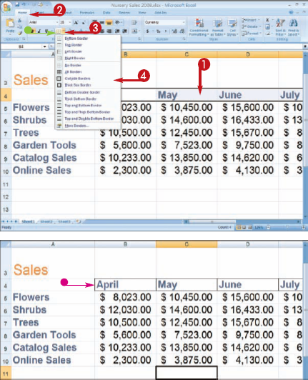
You can add borders to your worksheet cells to help define the contents or more clearly separate the data from surrounding cells. By default, Excel displays a grid format to help you enter data, but the borders defining the grid do not print.

You can add borders to all four sides of a cell, or choose to add borders to just one or two sides. Any borders that you add to the worksheet print along with the worksheet data.
Add Borders
ADD QUICK BORDERS

Note
See Chapter 9 to learn how to select cells.


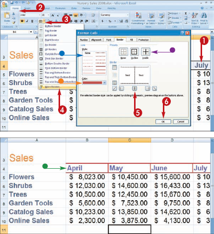
CREATE CUSTOM BORDERS

Note
See Chapter 9 to learn how to select cells.


The Format Cells dialog box appears with the Border tab displayed.

You can click multiple border buttons to create a custom border.


Note
Can I turn the worksheet gridlines on or off?
Yes. By default, Excel displays gridlines to help you differentiate between cells as you build your worksheets. You can turn gridlines off to view how your data will look when printed. Click the Page Layout tab on the Ribbon. Under the Sheet Options group, click the View check box for gridlines (

How do I add color inside my worksheet cells?
You can click the Fill Color

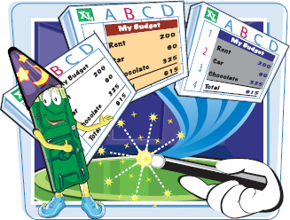
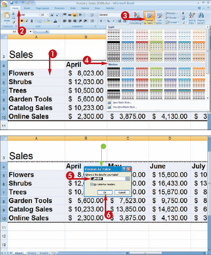
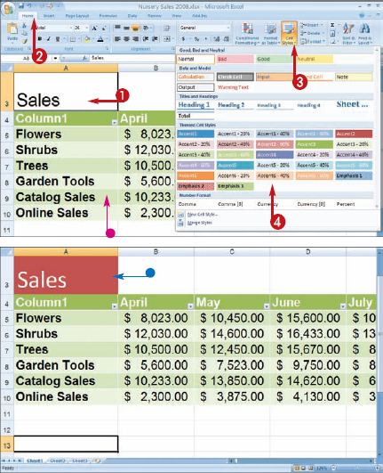
You can use Excel's Styles to apply preset formatting designs to your worksheet data. You can apply table styles to a group of worksheet data, or you can apply cell styles to individual cells or ranges of cells. When you apply a table style, Excel converts the data into a table.
Format Data with Styles
FORMAT AS A TABLE

Note
See Chapter 9 to learn how to select cells.


APPLY A CELL STYLE

Note
See Chapter 9 to learn how to select cells.


Note
Can I add a background to my spreadsheet?
Yes. You can add a background picture to any sheet. To do so, click the Page Layout tab on the Ribbon and click the Background button. This opens the Sheet Background dialog box, in which you can navigate to the picture that you want to use. Be very careful when applying background images to your worksheet, and ensure that the image does not distract from the legibility of your cell data.

How do I apply a theme?
You can use themes to create a similar appearance among all of the Office documents that you create. Themes are shared through Word, PowerPoint, and Excel. To apply a theme to your spreadsheet, simply click the Page Layout tab on the Ribbon, click the Themes button, and then select a theme from the list. You can use the Colors, Fonts, and Effects tools to fine-tune a theme.

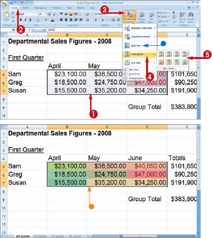
You can use color scales and data bars as additional visual guides to help you distinguish which cells meet your conditional rules.

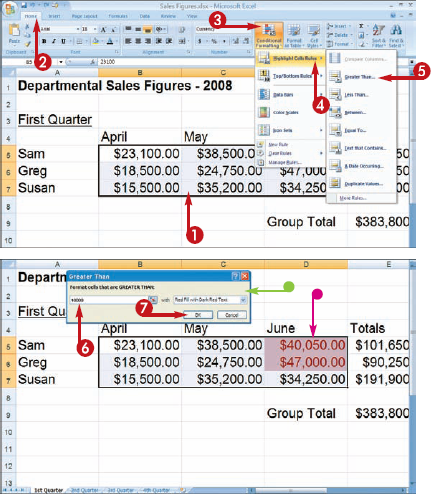
You can use Excel's conditional formatting feature to assign certain formatting only when the value of a cell meets the required condition. For example, your worksheet may track weekly sales and compare them to last year's sales during the same week. You can set up conditional formatting to alert you if a sales figure falls below last year's level, and make the cell data stand out among the other cells.
Assign Conditional Formatting
APPLY A CONDITIONAL RULE
APPLY A COLOR SCALE
Note
How do I create a new rule for conditional formatting?
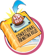
You can open the New Formatting Rule dialog box to set a new rule and formatting for the condition that you set. Click the Conditional Formatting button on the Home tab, and then click New Rule to open the dialog box. Use the dialog box to define the condition of the rule, as well as what formatting you want to apply when the condition is met.
How do I remove conditional formatting from a cell?
To remove conditional formatting, you can use the Conditional Formatting Rules Manager dialog box. Select the data, click the Conditional Formatting button on the Home tab, and then click Manage Rules. Next, click the rule that you want to remove, and click Delete Rule.
