When working with Access for the first time, it is tempting to start filling tables right away and querying data to get fast results, but it's important to understand the basics of the relational database concept before pounding away at data. A good understanding of how a relational database works will help you take full advantage of Access as a powerful data analysis solution. This chapter covers the fundamentals of Access and methods to bring data into the program.
Upon opening any existing Access database, you notice that the Database window, shown in Figure 2-1, contains a task pane on the left. Using the topmost dropdown box, change the navigation category to All Access Objects. You will get six sections. Each section represents one of the six database objects: Tables, Queries, Forms, Reports, Macros, and Modules. The Tables section is appropriately at the top of the list because it is the precise location where your data will be stored. All other database objects will refer to the tables in your database for data, whether asking questions of the data or creating reports based on the data. This section covers the basics to get you working with Access tables.
One way to think of a table is as a collection of data concerning a specific type of entity (such as customers, branches, transactions, products, and so on). You want each of these entities to have its own unique table. Among the many advantages to storing your data using this approach is eliminating or significantly decreasing duplicate information. Later in this chapter, you will learn about the dangers inherent in storing data with excessive duplications.
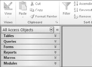
Figure 2.1. The navigation pane on the left allows you to navigate through the six types of database objects: Tables, Queries, Forms, Reports, Macros, and Modules.
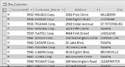
Open your sample database and go to the Tables section in the navigation pane. Double-click the Dim_Customers table. When the table opens, it is in the Datasheet view. In this view, you are able to directly view and edit the contents of the table. As you can see in Figure 2-2, the names of the columns are at the top.
A table is composed of rows, with each row representing an individual entity. In the Dim_Customers table, each row represents a single distinct customer. The proper database terminology for a row is record.
A table is also composed of columns, with each column representing a particular piece of information common to all instances of the table's entities. In Dim_Customers, each column represents some attribute of the customer record. The proper database terminology for a column is field.
Tip
The number of records in a table is visible at the bottom left of the Datasheet view, next to the record selectors.
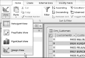
Through the Design view of a table, you are able to set the field names and data types. To get to the Design view of the Dim_Customers table, go to the Home tab and select View
As you can see in Figure 2-4, the Design view shows you the fields that compose the Dim_Customers table in an easy-to-manage view.
Note how each field has a Field Name and a Data Type. The Field Name is the descriptive text string given to that particular column of a table. It appears at the top of the table when it is in the Datasheet view. The Data Type of the field ensures that only a certain type of data is allowed in the field. If a data type is tagged as a Number, Access does not allow any text to be entered into that field. By setting the data type of each column, you go a long way toward ensuring the integrity and consistency of the data.
Tip
It's good practice to avoid putting any spaces in your field names. When constructing queries or referring to tables in VBA code, spaces in the field names can lead to problems. If you need to indicate a space in your field name, use the underscore character. Keep in mind that your field names cannot include a period (.), an exclamation point (!), an accent grave (`), or brackets ([ ]).
With the Design view of the Dim_Customers table open, select the Data type section of the first field and click the drop-down arrow. A list of predefined data type choices becomes visible. These data types are Text; Memo; Number; Date/Time; Currency; AutoNumber; Yes/No; OLE Object; Hyperlink; Attachment; and Calculated.
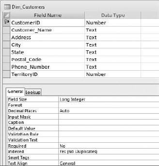
Figure 2.4. Opening the table in the Design view allows you to add field names or change existing ones.
Note
When in Design View, you will also see a data type selection called Lookup Wizard. This selection is actually not a data type at all; it's a mechanism used to activate the Lookup Wizard in order to create lookup fields. The Lookup Wizard is beyond the scope of this book.
Text: Any combination of letters, numbers, spaces, and characters is text. This is by far the most common data type. Although text can be a number, it should not be a number used in a calculation. Examples of common uses of the Text data type are customer names, customer numbers (using customer numbers in calculations would have no meaning), and addresses. The maximum number of characters allowed in a Text field is 255 characters.
Memo: If you need to store text data that exceeds the 255-character limit of the Text field, the Memo field should be used. Long descriptions or notes about the record can be stored in fields of this type.
Number: This type is for all numerical data used in calculations, except currency (which has its own data type). Actually, Number is several data types under one heading. When you select Number as a data type in the Design view of the table, you go to the Field Size field at the top of the General tab. When you select the drop-down arrow, you get the following options: Byte, Integer, Long Integer, Single, Double, Replication ID, and Decimal. Probably the most commonly used field sizes of the Number data type are Long Integer and Double. Long Integer should be selected if the numbers are whole numbers that do not have any non-zeros to the right of the decimal point. Double should be selected if numbers with decimals need to be stored.
Date/Time: Another data type often used in calculations is Date/Time. Recording the time that certain events occur is among the more important uses of this data type. Recording dates and times allows you to compare data by time durations, be it months, years, or whatever. In the business world, the date field can be crucial to analysis, especially in identifying seasonal trends or year-over-year comparisons.
Currency: A special calculation data type, Currency is ideal for storing all data that represents amounts of money.
AutoNumber: This data type is actually a Long Integer automatically and sequentially created for each new record added to a table. The AutoNumber can be one mechanism by which you can uniquely identify each record in a table. You will not enter data into this field.
Yes/No: There are situations where the data that needs to be represented is in a simple Yes/No format. Although you could use the Text data type for creating a True/False field, it is much more intuitive to use Access's native data type for this purpose.
OLE Object: This data type is not encountered very often in data analysis. It is used when the field must store a binary file, such as a picture or sound file.
Hyperlink: When you need to store an address to a Web site, this is the preferred data type.
Attachment: This data type was introduced with Access 2007. When you set a field to the Attachment type, you can attach images, spreadsheet files, documents, charts, and other types of supported files to the records in your database. You can also configure the field to view and edit attached files.
Calculated: This data type is new to Access 2010. With Calculated type fields, you can build mathematical operations, textual evaluations, or any other calculation directly into your table.
Access provides several methods for creating a table. The ideal way to create a table in Access is with the Design view. Why? The Design view allows for a compact work area so you can add fields, reposition fields, and assign attributes easily.
Imagine that the human resources department asks you to create a simple list of employees in Access.
To create this table in the Design view, go to the application ribbon and select the Create tab and then the Table Design button. This opens an empty table called Table1 in Design view.
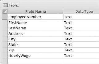
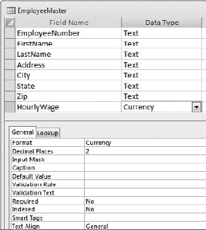
The idea here is to create a list of fields that describe employee attributes. Among the more common attributes in this situation are the following: EmployeeNumber, FirstName, LastName, Address, City, State, Zip, and HourlyWage. You begin by entering the names of the columns going down the list. When you have entered all of the required column names, your dialog box should look like Figure 2-5.
As you enter the field names, the data types default to the most common data type, Text. You now want to set the data type for each field or at least change the data type of each non-text field. Choosing the correct data type for the first field, EmployeeNumber, may be initially confusing. With the word "Number" in the field, you might think that Number would be the logical choice for the data type. Actually, the rule of thumb is that if the field will not be used in a calculation, it is best to set its data type to Text. Because there is no logical reason to perform a calculation on an employee's EmployeeNumber, the EmployeeNumber data type should remain Text. Another reason for using the Text data type for the field EmployeeNumber is that there could be a need to use alphabetic or other characters in the field.
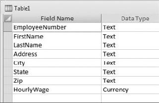
As you go through the field names, it should be fairly obvious that you will want to set all of the fields to Text, except for HourlyWage. This field will almost certainly be used in calculations, and it will represent a monetary value, so you should change the data type to Currency.
At this point, your Design view should look similar to Figure 2-6.
Now you can save and name your table. Click File on the application Ribbon and select Save As. If you are using Access 2007, click the Office Icon and select Save As. This opens the Save As dialog box where you will give your newly created table an appropriate name like "Employees" or "EmployeeMaster."
Keep in mind that at this point, this table has no data. You can begin entering employee information directly into the table through the Datasheet view. For tables with a small number of records, you can enter your records manually. However, most sets of data are quite large, so other techniques of bringing data into Access are introduced later in this chapter.
Note
When you save a table, you may be prompted to set a primary key. Primary keys are explained later (see Setting Primary Keys in this chapter). In most cases, Access will try to choose one for you. It's generally good practice to accept Access' recommendation to create a primary key if you do not already have one on mind.
When working with data in tables, you may encounter situations that require the data be restricted or to adhere to some default specifications in particular columns. You can define these requirements by using the field properties.
The field properties affect how the data is stored and presented, among other things. The list of field properties that are available to you is dependent on the data type chosen for that field. Some field properties are specific to Text fields, and others are specific to Number fields. The field properties can be found in the Design view, as illustrated in Figure 2-7. As you click on each field, you will see the field properties for that field.
Some of the most important field properties to note are:
Field Size: You encountered the Field Size before, when working with the Number data type. This property also exists for the common Text data type. This property allows you to set a maximum size limit on data entered in that column. For the Text data type, size refers to the length (number of characters and spaces) of the Text data in that column. For example, looking at the Employees table, you see a field for State. Your firm tells you that the names of states should be recorded using their two-letter designation. If you set the field size to "2" for the State column, the user will be unable to type any text that is longer than two characters. So with Access, you are not only able to force a certain data type in a particular column, you can also customize that individual column to accept data only in the rigid format that you specify.
Format: This property allows you to set the precise manner in which Access displays or prints the data that is located in its Tables. As with Field Size, the format available to select will depend on the data type of that column. For example, with a Currency field, you can display the data in a form that uses a dollar sign, a Euro sign, or no sign at all. With these settings, the data itself does not change—just how it displays. Another very useful function of Format is with Date/Time data types. Whether you want to display data in the long format or short format, this property allows you to set that option.
Input Mask: This feature can be useful in data entry situations. Where Format controls how data is displayed, Input Mask controls how data is entered into a particular field. Input mask is available for the following data types: Text, Number, Date/Time, and Currency. For example, if a user needs to enter a telephone number, the input mask can create the characters and structure with which you are all familiar. As the user types, the number automatically assumes a phone number format: (###) ###-####.
Decimal Places: In number fields, you can set the number of decimal places to the right of the decimal point that will be recorded. There is an Auto setting, which defers to the Format setting to determine the correct number of places. Apart from Auto, you are able to select 0 to 15 for the number of decimal places.
Default Value: An important database concept, the default value can help save time in the data entry process. The default value is automatically placed in that column every time a new record is added. Defaults can be overridden by simply entering data into the field.
Required: Another important property, Required simply forces a user to enter some value, using the proper data type, in the designated field. The user cannot add a new record if the Required field is not properly filled. As with Input Mask, this property is an excellent mechanism for asserting more control over the data entry process.
In some tables, you will need to ensure the uniqueness of each record. This is typically achieved by including a field whose records will not have duplicate values. One example of this is a field for Social Security numbers. Each person has one and only one unique Social Security number. By definition, you cannot have a Social Security number that represents two people. This type of unique column is what you call a primary key.
You can identify a given field as the primary key for you table in Design view—by right clicking the chosen field and selecting Primary Key. When you save your table, Access determines whether your selected fields have any null (or blank) values or duplicate data (data duplicating in multiple records for a single field). If there are blanks or duplicates, Access informs you with an error message. You must fill in the blanks with unique values and remove any duplicates if that column is indeed to become the primary key for the table.
Tip
Sometimes a table will have two or more fields that together uniquely identify a record. In these cases, you will need to create what is called a compound key. For example, imagine a table with both an invoice number and a product number. A sales representative may have sold multiple products to a customer on the same invoice. Therefore, when you look at each value separately, you'll find duplicate values of each field. By combining invoice and product number, however, you can create a compound primary key that is truly unique for each record. If you need a compound key, do the following:
Select the first field that will be included in your compound key by clicking on the grey square to the right of the Field Name. Then while holding down the Control key on your keyboard, click the grey square next to the second field to be included.
Right click on the Field Name (right clicking on the grey square will cause Access to forget your multiple selection).
Close the table and save your changes.
Apart from creating a table from scratch and manually entering the data, you can import data, which essentially makes a copy of the data directly in your Access database. After importing, the data is disconnected from the source from which it was imported.
To get an idea of how Importing works, imagine that HR has passed you an Excel file containing their master employee table. You want to import that table into your database.
Tip
The ExcelMaster.xlsx file can be found within the sample files for this book, installed under C:OffTheGrid.
Click the External Data tab and then click the Excel icon.
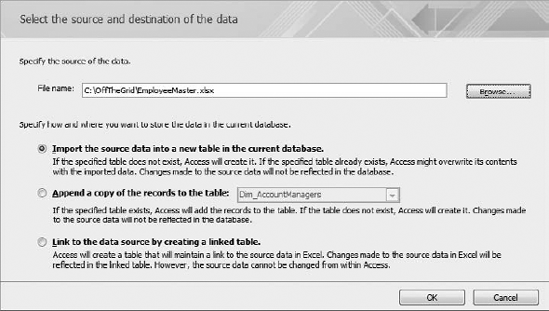
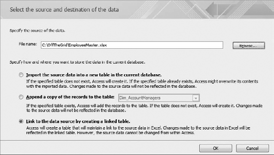
Browse for the file you wish to import and then select the "Import the source data into a new table..." option. Figure 2-8 shows you what the wizard should look like.
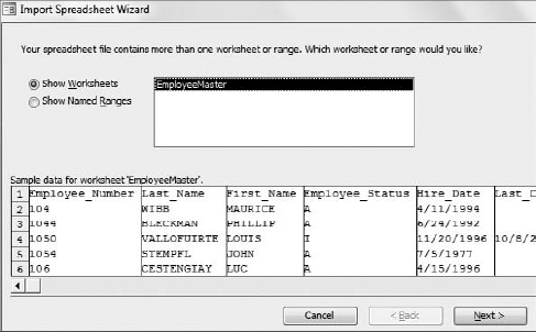
Click the OK button to activate the Import Spreadsheet Wizard shown in Figure 2-9. The first dialog box in the Import Spreadsheet Wizard allows you to specify the worksheet or range you want to import. If your workbook has more than one worksheet, all worksheets are listed on this screen. In this case, there is only one worksheet. Select the target worksheet and click the Next button.
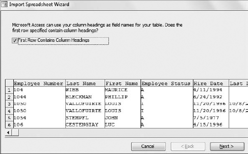
The next screen (Figure 2-10) allows you to select whether or not the source data has headings or column labels. As you can see, you will simply check the checkbox if your source data has headings. Click the Next button to move on.
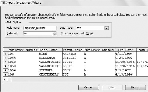
The next screen (Figure 2-11) allows you to specify the data type for each field. This setting allows you to tell Access whether the given field is a number, text, currency, date, etc. The idea is to select each field and check to make sure the data type for that field is correct.
Also in this screen (Figure 2-11), you can specify whether any given field is to be indexed. When you index a field, Access creates a kind of organizational mapping of the field allowing for faster querying and grouping.
The best way to illustrate indexing is by an analogy. Imagine you had a file cabinet with 10,000 folders, each dedicated to a specific customer. Now imagine these files were in random order. To access the customer file for "Mike's Coffee House," you would have to search through every customer file until you found it. Now imagine finding the file if your customer folders were organized or "indexed" alphabetically. It would be a much faster task. When you sort or filter on a non-indexed field, Access will search every record until the correct record is found. Indexing a field in Access is conceptually identical to alphabetizing the file system. Indexing a field makes Access create an organizational scheme for that field such that it can be quickly searched when needed.
Note
You may wonder why you would not index all your fields. Wouldn't that make your queries run faster? The answer is an emphatic no! Indexing is a good idea on fields you expect to filter or join to another table. Indexing is not a good idea for fields you expect to perform calculations on. You should also be aware that while indexing can improve the performance for some types of analysis, other types could actually be slowed by using indexed fields.
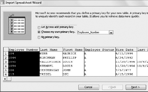
Clicking Next will bring you to the screen shown in Figure 2-12. Here, you can choose the field to set as the primary key. In this case, the Employee_Number field will be primary key.
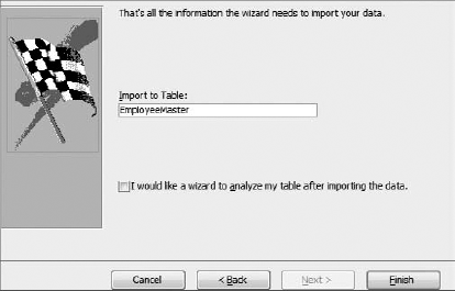
The last screen of the Import Spreadsheet Wizard (Figure 2-13) will ask to you name your new table. If you are importing an Excel worksheet, the new table name will default to the name of your imported worksheet. However, you can change the name to suit your needs. At this point, you can click the Finish button to start the import.
Note
It's important to note that naming your import table the same name as an existing table in your database will cause Access to give you an overwrite warning. That is to say, Access will warn you that you are about to overwrite your existing table. Be careful that you do not inadvertently overwrite an existing table with a careless table name choice.
Once your data has been imported, an interesting dialog box activates (Figure 2-14). This dialog box asks if you want to save your import steps. This is a relatively new feature introduced in Access 2007, allowing you to save time when the same dataset must be routinely imported. As you can see in Figure 1-14, clicking the "Save import steps" option allows you to save your import steps as a named task that can be fired whenever you need. To recall a saved import task, simply click the Saved Imports command button under the External Data tab in the Access ribbon.
You may want to import and analyze non-Excel data and then send it to Excel after analysis in Access. One of the most common data types for import is text-delimited data. Delimited text is simply text where the individual fields in a record are separated by a specific character such as a tab, comma, or space.
Fortunately, Access recognizes delimited text and even allows you to choose the specific character that separates fields. To get delimited text into Access, simply choose Text File from the External Data ribbon and walk through the same process you would when importing or linking to an Excel file.
Sometimes, the data you want to incorporate into Access is going to change frequently. Does it make sense to import that data into a new Access table every time it changes? What if you do not know when it changes yet it is critical to have the most up-to-date information for your analysis? In these situations, it makes more sense to create a link to your data.
Linking data is different from importing data in that Access references the linked data in its original location. Importing data brings a local copy of the information into the Access database. Any changes made to the local copy in Access do not affect the original spreadsheet. Likewise, any changes made to the original spreadsheet after importing will not be reflected in the Access table.
Conversely, a linked Excel sheet exists in real time. Changes made to the sheet in the original Excel file will be reflected in Access upon refresh. However, you will not be able to make changes to the Excel data through Access. Linking is a one-way street of data flow.
To link to a data source, you would start by selecting the External Data tab and then select the Import Excel icon. This time, select the "Link to the data source by creating a linked table" option (see Figure 2-15).
From here, Access will walk you through steps similar to those taken when importing data.
Note
When linking to a data source, you will not be able to specify data types, indexing, or primary keys. Therefore, you will not see those selections in the Link Spreadsheet Wizard.
Now that you have covered tables and brought some data into the database, you can turn your focus to one of the more useful features of Access: relationships. Access relationships are the mechanisms by which separate tables are related to each other. The idea behind relationships is the Relational Database Concept. Before you begin to create relationships between Access tables, take a closer look at the concept behind relational database systems.
This concept is important because it is the theoretical framework from which most databases programs are designed. If you want to understand just how databases work, you need to understand this concept. You are learning Access, among other reasons, because the data storage and data manipulation capacity of Excel is insufficient for your analysis needs.
The concept that dictates just how data is stored and structured is the Relational Database Concept. Even though you may have no intention of becoming a database administrator, having some understanding of how the data that you would like to analyze has been stored and structured will increase your performance and productivity. It will also promote better communication between you and the IT department and the database administrator, since now you will be able to understand at least some of the vocabulary of the database language.
Before you cover the proper techniques for storing data in Access, examine the common data storage scenario that led to the problems that the concept attempts to address. Even if they are not aware of the term flat-file format, most Excel users are very adept at working with data that has been stored in it. In fact, most people are familiar with the concept because it is used in so many things that they encounter every day. The flat-file, of course, organizes data into rows and columns.
There are data analysis scenarios that are not terribly complex, in which a flat-file representation of the data to be analyzed is adequate. However, most data-analysis scenarios require analyzing data that is much more multi-dimensional. One of the main reasons that the flat-file can prove inadequate is that it is two-dimensional. Real-world business data rarely falls into a convenient, two-dimensional format. Of course, it can be forced into that format by the Excel guru who wants all analysis to fit into the spreadsheet.
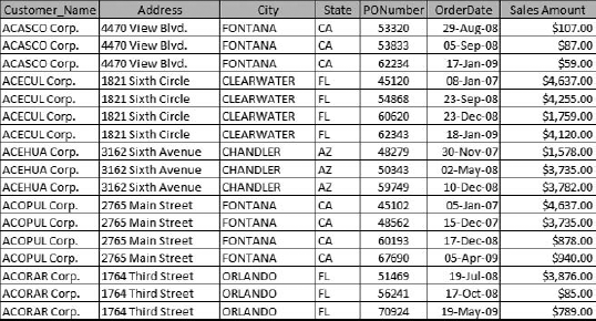
Take a look at a typical example of a flat-file; Figure 2-16 shows a typical flat-file list of orders.
In order to get the customer information for each order, there are several fields for customer-specific information such as customer name, address, city, and so on. Because most firms sell to customers more than once, for each order the same customer information has to be repeated. Duplicate information is one of the main drawbacks of the flat-file format.
What is wrong with duplicate data? Initially, the duplicate data may not appear to be a potential source of future problems, but upon further examination, you discover the shortcomings:
File Size. Duplicate data wastes space, both on the computer hard drive, where the file is stored, and in the computer's memory, where the data resides when it is being used. Although the enormous amount of memory that is standard with today's machines goes a long way to handling these demands, you are wasting valuable computer space and resources. The duplicate information is not valuable. In fact, it leads to problems.
Updating data: One of the main problems that can arise from too much duplicate data occurs when that data needs to be updated.
In Figure 2-16, you can see there are several orders for ACASCO Corp. You can also see that you have to repeat the information about the customer for each instance of an order. Imagine a scenario where the customer information might change. For example, the customer acquires new office space, and you want to reflect this change of location in your data. You will have to update the change in several different places. You need to ensure that every order will correctly map back to its relevant customer information.
While there are excellent functions that find and replace data in Excel, there is still a danger that you might not make all of the updates correctly. Whenever you are changing duplicate information, there is always the risk of introducing unintentional errors.
Data must be consistent if analysis is to have any true value in the decision-making process. Duplicate data is the bane of consistent data. If an entity is changed in one place, it must be changed in every place. Would it not be more logical and efficient if you could create the name and information of a customer only once? Would it not be great simply to have some form of customer reference number instead of creating the same customer information repeatedly? Then that customer reference could send you to another list where the information is unique and written once.
This is the idea behind the relational database concept. You have separate, carefully designed, unique lists of data, and you relate them to each other by using their unique identifiers (primary keys).
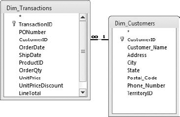
In a relational database, customer details such as address, city, state, etc, would be listed only once in a master customer table. A transactions table using a primary key such as CustomerID would then reference that table (Figure 2-17). This way, if any of the details for a given customer were to change, edits would have to be applied only to that customer's one record in the master customer table.
Excel users may not realize it, but they often make great efforts to keep the data on their spreadsheets "relational." They use (or overuse) VLOOKUP or HLOOKUP to match data from separate lists that have some data field or key in common. While much is possible with these functions, they do have their limitations. The functions are not very intuitive and try to solve a problem that Access was designed, from the ground up, to address. When Excel users use functions like VLOOKUP and HLOOKUP to bring data from separate lists onto a single row, they are emulating a relationship of that data.
The problem for the analyst is that if there are relationships between the data that are consistent or even permanent, it is easier somehow to reflect this in a behind-the-scenes representation of the data. Some of the data relationships can be quite complex, which compels the analyst to remember and manually enforce all of them but also detracts from analysis and increases the possibility of mistakes.
Three types of relationships can be set in a relational database:
One-to-one relationship: For each record in one table, there is one and only one matching record in a different table. It is as if two tables have the exact same primary key. Typically, data from different tables in a one-to-one relationship are combined into one table.
One-to-many relationship: For each record in one table, there may be 0, 1 or many records matching in a separate table. For example, you might have an invoice header table related to an invoice detail table. The invoice header table has a primary key, Invoice Number. The invoice detail table will use the Invoice Number for every record representing a detail of that particular invoice. This is certainly the most common type of relationship you will encounter.
Many-to-many relationship: Used decidedly less often, this relationship cannot be defined in Access without the use of a mapping table. This relationship states that records in both tables can have any number of matching records in the other table.
In the sample database that came with this book, relationships have already been established between the tables. Take a look at some of these relationships to get a better idea of how you can set and change them.
In Access 2007, go up to the application ribbon and select the Database Tools

In Access 2010, go up to the application ribbon and select File

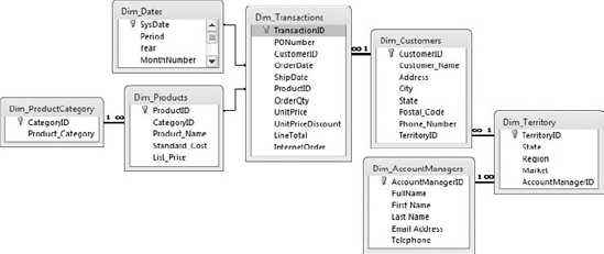
As you can see in Figure 2-18, the tables are represented with lines between them. The lines signify the relationships.
Once you have a fundamental understanding of tables and relationships in Access, you are ready to start analyzing data with queries. In this section, you are going to focus on what is perhaps the most common type of query: the select query. You will see the concept behind the query and a few examples that illustrate just how easy it is to create queries in Access.
By definition, a query is a question. For your purposes, it is a question about the data, which is stored in tables. Queries can be exceedingly simple, like asking what all of the data in a table is. Queries can also be quite complex, testing for different criteria, sorting in certain orders, and performing calculations. In Access, there are two main types of queries: select and action:
Select queries are perhaps the most common type. This query simply asks a question of the data and returns the results. No changes are made to the data whatsoever. You can always run select queries and never worry that the actual data is being altered.
Action queries actually manipulate and change the data in a table. The action query can add records, delete records, or change (update) information in existing records.
Quite often, when you are working with or analyzing data, it is preferable to work with smaller sections of the data at a time. The tables contain all the records pertaining to a particular entity, but perhaps for your purposes you need to examine a subset of that data. Typically, the subsets are defined by categories or criteria. The select query allows you to determine exactly which records will be returned to you.
If you thought that creating queries required learning a programming language or some other technological hurdle, you are mistaken. While it is possible to create queries using the programming language of databases (SQL), Access provides a graphical interface that is easy to use and quite user-friendly. This graphical interface has been called the QBE (Query by Example) or QBD (Query by Design) in the past. Now Microsoft calls it the Query Design view. In the Query Design view, tables and columns are visually represented, making it easy to visualize the "question" you would like to ask of the data.
Follow these steps:
Go up to the application ribbon and select Create

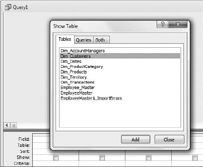
When creating your "question" of the data, the first thing you must determine is from which tables you need to retrieve data. The Show Table dialog box allows the user to select one or more tables. As you can see in Figure 2-21, there are also tabs for Queries and Both. One of the wonderful features of queries is that you are not limited to just querying directly from the table. You can create queries of other queries.
For this first query, select the Dim_Customers table, either by selecting the table in the list and clicking Add or by double-clicking the table in the list. Now that you have selected the table from which you want to retrieve data, you can close the Show Table dialog box and select the fields of that table that you would like to retrieve.
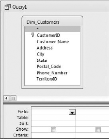
The Query Design view is divided into two sections. The top half shows the tables or queries from which the query will retrieve data. The bottom half (often called the query grid) shows the fields from which the query will retrieve data. You will notice in Figure 2-22 that the Dim_Customers table shown at the top half of the Query Design view lists all the fields but has an asterisk at the top of the list. The asterisk is the traditional database symbol that means that all fields from that table will be in the output.
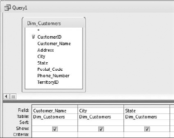
For this example, select the following three fields: Customer_Name, City, and State. To select fields, you can either double-click the field or click it once and drag it down to the bottom half (the query grid). Each field that you add to the query grid will be included in the output of the query. Figure 2-23 shows you how your query should look after selecting the output fields.
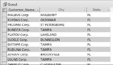
At this point, you have all you need to run the query. To run the query, click the Run button located on the Design tab. As you can see in Figure 2-24, the output from a query looks similar to a regular table after it is open.
Note
To return to the Query Design view, simply click Home
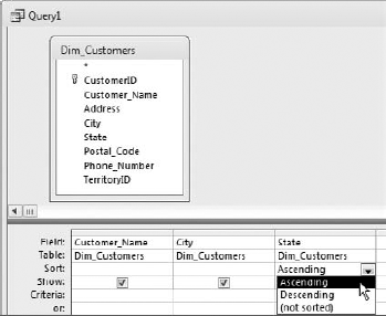
Now examine how you can sort the results of this query. Just as you sorted in Excel, you are going to select a column and choose between an ascending sort and a descending sort. In the query grid, notice the Sort row of the grid. This is where you can select either one or multiple sort columns. If you select multiple sort columns, the query will sort the results in order from left to right.
Go to the State column and click your mouse on the Sort section. As shown in Figure 2-25, a dropdown box appears, allowing you to select either Ascending or Descending for that particular column.
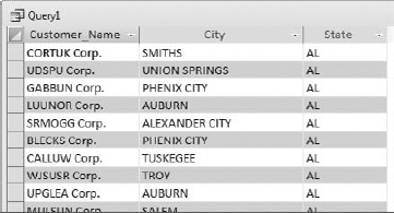
Select Ascending and rerun the query. When you ran the query before, the states were in no particular order. After setting the sort order of the State column to ascending, the query output simply looks better and more professionally formatted, as seen in Figure 2-26.
Next, you'll examine how you can filter the query output so that you retrieve only the specific records to analyze. As in Excel, in Access this filter is also called Criteria.
Note
You will notice a Criteria row in the query grid. This is where you enter the value or values for which you would like to query. When entering a value in the Criteria section, all records that match it are returned in the query output. When entering text, you must enclose the text string with quotation marks. You can either place them there yourself or type your text and click another part of the query grid. Access then automatically places quotation marks around your criteria if the field you are filtering is a text field.
In the example demonstrated in Figure 2-27, your manager wants to see the list of customers from California. Since California is designated bythe abbreviation "CA" in the table, that is exactly what you will enter in the Criteria row of the State column.
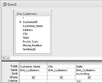
Figure 2.27. The Criteria section is where you type in a value for which you want to filter the data.
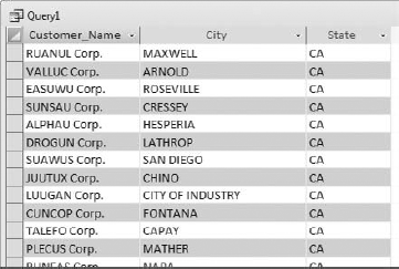
After you run the query, you will notice that fewer records are returned. This is obvious from looking at the Record Selector at the bottom of the query output window. A quick scan of the results verifies that indeed only records with "CA" in the State column were returned, as shown in Figure 2-28.
Tip
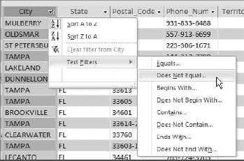
You can sort and filter query results just as if they were a Table. Simply click the dropdown arrow next to each of the column headings to activate the sorting and filtering context menu. Remember, this is only temporary and does not affect the underlying query.
In this section you'll see how you can perform a query on multiple tables. Remember that you split your data into separate tables. You used Relationships to define the logical relationships between the data. Now you will query from the tables based on the relationships established.
For example, say you want to see the customer transactions from California. A quick examination of the Dim_Transactions table reveals that there is no State field on which you can filter. However, you see that there is a CustomerID field. Follow these steps:
In the query that you already have opened, add the Dim_Transactions table so you can include some fields from that table in your query output.
Right-click the top half of the Query Design view and select Show Table.
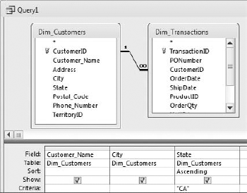
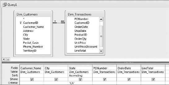
Double click the Dim_Transactions table to add it to the Query Design view. You will notice that the previously established relationship is automatically represented, as shown in Figure 2-29. You can see the one-to-many relationship, indicating possible multiple records in Dim_Transactions for each individual customer in the Dim_Customers table.
You must now select the fields from your newly added table, which you need to appear in the query output. Select the following three fields from the Dim_Transactions table: PONumber, OrderDate, LineTotal. As you can see in Figure 2-30, the field names from the two tables are brought together in the query grid.
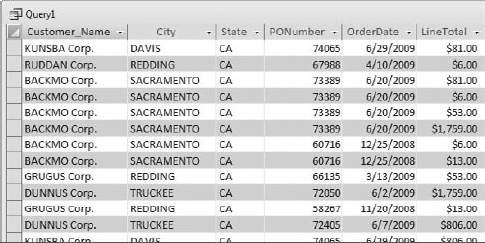
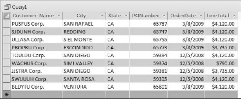
As you can see in Figure 2-31, you now have orders matched with the appropriate customer data. Although there is repeating data, as with the flat-file examples, there is a significant difference. The repeating data is being read from a single source, the Dim_Customer table. If a value were to change in the Dim_Customer table, that changed value would be repeated in your query results.
You can narrow your results even further by filtering the query results according to a certain date. As you can see, there are several rows of criteria cells. These allow you to enter multiple criteria from which to filter. One thing to keep in mind is that each separate criteria row functions as its own separate set of criteria. Take a look at how this works.
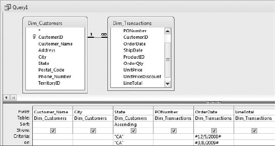
Single Criterion: Click the Criteria cell in the OrderDate column and type 12/5/2008. When you click out of that cell, you will notice that number signs (#) now surround the date, as shown in Figure 2-32. When running this query, only results matching the two criteria (State = CA and Invoice_Date = 12/5/2008) are returned.
Multiple Criteria: Say you want to bring in orders for the data 3/8/2009 as well as 12/5/2008. You will want to add the new criteria line below the existing criteria. This will have the effect of testing the records for either one criteria or the other. Since you want to limit your query to only results from California, you must retype CA on your new Criteria line. If you do not do that, the Query will think that you want all orders from California on 12/5/2008 or orders from all states on 3/8/2009. The criteria lines will be evaluated individually. Add CA to the state column under the existing CA, as shown in Figure 2-33.
After running the query, you can see your results have been refined even further. You have only those orders from California issued on March 9, 2009 and December 5, 2008.
To use multiple criteria in a query, you are not limited to using the separate criteria lines. By using operators, you can place your multiple criteria on the same line. That is to say, you can filter for multiple criteria on any given field by using operators.
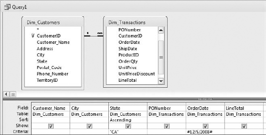
Figure 2.32. The number signs, which are surrounding the date, identify the criteria as being a Date/Time data type.
The following operators allow you to combine multiple values in different logical contexts so you can create complex queries:
Or: Either condition can be true. Multiple criteria values for one field can either be separated on different criteria lines or combined in one cell with the use of the
Oroperator. For example, using your query, you can filter for both California and Colorado by typing CA or CO in the Criteria field.Between: Tests for a range of values. For example, using your query, you can filter for all orders between 4/20/2009 and 11/19/2009 instead of testing just for those particular dates by typing Between #4/20/2009# AND #11/19/2009# in the Criteria field.
Like: Tests for string expressions matching a pattern. For example, you can filter for all records with a customer ID that begins with the number 147 by typing Like 147* in the Criteria field. The asterisk is the wild card character, which can signify any character or combination of characters.
In: Similar to
Or. Tests for all records that have values, which are contained in parentheses. For example, you can filter for both California and Colorado by typing In ("CA", "CO") in the Criteria field.Not: Opposite of writing a value in Criteria. All records not matching that value will be returned. For example, you can filter for all states except California by typing Not "CA" in the Criteria field.
Is Null: Filters all records that have the database value Null in that field.
=, <, >, <=, >=, and <>: The traditional mathematical operators allow you to construct complex criteria for fields used in calculations.
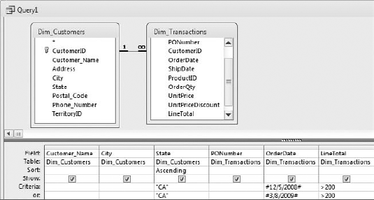
For example, suppose you want to further refine your query so that only order amounts over $200 will be returned in the results. As shown in Figure 2-34, use the greater-than operator to filter the LineTotal.
After running the query, you can see that you narrowed your results down to just nine records. These are the only records that match the multiple criteria designated in the query grid. Figure 2-35 shows the query results.
When starting to build analyses with Access, you will inevitably do something that makes Access throw up an error. In order to ease the confusion when first starting out, Table 2-1 and Table 2-2 list the ten most common errors new users are likely to encounter while working with queries. The tenth error deservers a table all of its own! Ironically, although these are the most common errors in a query environment, they are also the least descriptive. This leaves many new Access users scratching their heads.
Table 2.1. Top Nine Query Errors
The error messages "Operation must use an updateable query" and "This Recordset is not updateable," are thrown when any of the queries in Table 2-2 are applied.
Table 2.2. Tenth Query Error, 3073 and 3326
The fundamental tools in Access are tables and queries. A table is a collection of data concerning a specific types of entities such as customers, branches, transactions, and products. Access allows you to build relationships between your tables and enforce certain rules that guide these relationships. This reduces the chance for error and allows for easy analysis across multiple tables.
A query is a question about the data that is stored in tables. The results of a query are separate from the data. If the data in the table is changed and the query run again, you would most often get different results. The most common query is the select query. With a select query, you can extract a dataset or individual data items. You can also utilize the built-in operators to apply filters and sorting to your queries.

