CHAPTER 4

Non-Parametric Analysis of Rating Transition and Default Data

Peter Fledelius,^a David Lando,^b,* and Jens Perch Nielsen^a

1. INTRODUCTION

The key purpose of rating systems is to provide a simple classification of default risk of bond issuers, counterparties, borrowers, and so on. A desirable feature of a rating system is, of course, that it is successful in ordering firms so that default rates are higher for lower-rated firms. However, this ordering of credit risk is not sufficient for the role that ratings are bound to play in the future. A rating system will be put to use for risk management purposes, and the transition and default probabilities associated with different ratings will have concrete implications for internal capital allocation decisions and for solvency requirements put forth by regulators. The accuracy of these decisions and requirements depends critically on a solid understanding of the statistical properties of the rating systems employed.

It is widely documented that the evolution of ratings displays different types of non-Markovian behavior. Not only do there seem to be cyclical components but there is also evidence that the time spent in a given state and the direction from which the current rating was reached affects the distribution of the next rating move. Even if this is consistent with stated objectives of the rating agencies (as discussed below), it is still of interest to quantify these effects since they improve our understanding of the rating process and of the forecasts one may wish to associate with ratings.

In this chapter, we use non-parametric techniques to document the dependence of transition intensities on duration and previous state. This exercise serves two key purposes. First, we show that these effects can be more clearly demonstrated in a non-parametric setting where the specific modeling assumptions are few. For example, we find that the effect of whether the previous move was a downgrade or an upgrade vanishes after about 30 months since the last move but that it is significant up to that point in time. We also consider stratification of firms in a particular rating class according to the way in which the current rating class was reached, reinforcing the results reached, for example, in Lando and Skødeberg (2002). Again, we are able to quantify how long the effect persists. To do this requires a notion of significance and we base this on the calculation of pointwise confidence intervals by a bootstrap method, which we explain in this chapter.

The second purpose is to point more generally to the non-parametric techniques as a fast way of revealing whether there is any hope of finding a certain property of default rates or transition probabilities in the data, how to possibly parameterize this property in a parametric statistical model, and even to test whether certain effects found in the data are significant using a non-parametric confidence set procedure. We illustrate this from beginning to end, keeping our focus on a single rating class and jointly modeling the effects of the previous rating move, duration in the current rating, and calendar time.

While the technique is used to examine only a few central issues in the rating literature, it is clear that the methods can be extended to other areas of focus. For example, the question of whether transitions depend on economic conditions, key accounting variables for the individual firms, and other covariates may also be addressed. Whatever the purpose, the non-parametric techniques used in this chapter combined with the smoothing have two main advantages. First, whenever we formulate hypotheses related to several covariates, there is a serious thinning of the data material. Consider, for example, what happens if we study downward transitions from a rating class as a function of, say, calendar time t and duration since last transition x. In this case, we have not only limited our attention to a particular rating class, but for every transition that occurs, we also have a set of covariates in two dimensions (calendar time and time in state) and we wish to say something about the dependence of the transition intensities on this pair of covariates. This inevitably leads to a “thinness” of data. The smoothing techniques help transform what may seem as very erratic behavior into a recognizable systematic behavior in the data. In this way, even if we have been ambitious in separating out the data into many categories and to a dependence of more than one covariate, we are still able to detect patterns in the data—or to conclude that certain patterns are probably not in the data. The pictures we obtain can be much more informative than a parametric test. Second, if we detect patterns in the data, we may often be interested in building parametric models. With more dimensions in the data, tractability and our ability to interpret the estimators require some sort of additive or a multiplicative structure to be present in these parametric models. The methods employed in this chapter allow one not only to propose more suitable parametric families for the one-dimensional hazards, but they also help detect additive or multiplicative structures in the data using a technique known as marginal integration.

In essence, marginal integration gives us non-parametric estimators for the marginal (one-dimensional) hazard functions based on a joint multivariate hazard estimation. The idea is to first estimate the joint hazard and then marginally integrate. If an additive or multiplicative structure is present, this integration gives the marginal intensities and—very importantly—these estimators of one-dimensional hazards are not subject to problems with confounding factors. To explain what we mean by this, consider a case where there are two business cycle regimes, one “bad” with a high downgrade intensity from a particular state and one “good” with a low intensity. Assume that we are primarily interested in measuring the effect on the downgrade intensity of duration, that is, time spent in a state. If the sample of firms with short duration consists mainly of firms observed in the bad period and the sample of firms with long duration consists mainly of firms observed in the good period, then a one-dimensional analysis of the downgrade intensity as a function of duration may show lower intensities for long duration even if this effect is not present in the data. The effect shows up simply as a consequence of the composition of the sample and is really due to a business cycle effect. In our analysis, this problem is avoided by modeling the intensity as a function of calendar time and duration and then finding the contribution of duration to the intensity through marginal integration.

The main technical aspect of this chapter is the smoothing technique itself. For the reader interested in pursuing the statistical methods in more depth, we comment briefly on the related literature from statistics. Throughout this study we use the so-called “local constant” two-dimensional intensity estimator developed by Fusaro et al. (1993) and Nielsen and Linton (1995). This local constant estimator can be viewed as the natural analogue to the traditional Nadaraya–Watson estimator known from nonlinear regression as a local constant estimator; see Fan and Gijbels (1996). We could have decided to use the so-called “local linear” two-dimensional intensity estimator as defined in Nielsen (1998). This would have paralleled the development in regression, where local linear regression is widely used, primarily due to its convenient properties around boundaries; see Fan and Gijbels (1996). However, our primary focus is an introduction of these novel non-parametric techniques to credit rating data. We have, therefore, decided to stick to the most intuitive procedures and avoid any unnecessary complications.

Rating systems have become increasingly important for credit risk management in financial institutions. They serve not only as a tool for internal risk management but are also bound to play an important role in the Basel II proposals for formulating capital adequacy requirements for banks. Partly as a consequence of this, there is a growing literature on the analysis of rating transitions. To our knowledge, the first literature to analyze non-Markovian behavior and “rating drift” are Altman and Kao (1992a–c) and Lucas and Lonski (1992). Carty (1997) also examines various measures of drift. The definitions of drift vary, but typically involve looking at proportions of downgrades to upgrades either within a class or across classes.

It is important to be precise about the deviations from Markov assumptions. It is perfectly consistent with Markovian behavior, of course, to have a larger probability of downgrade than upgrade from a particular class. In this chapter we are not concerned with this notion of “drift.” Rather, we are interested in measuring whether the direction of a previous rating move influences the current transition intensity. We are also interested in measuring the effect of time spent in a state on transition intensities. Note that variations in the intensity as a function of time spent in a state could still be consistent with time non homogeneous Markov chains, but the marginal integration technique allows us to filter out such effects related to calendar time (or business cycles) and show non Markovian behavior. The non-parametric modeling of calendar time is similar to that of Lando and Skødeberg (2002), where a semiparametric multiplicative intensity model, with a time-varying “baseline intensity,” is used to analyze duration effects and effects of previous rating moves. There the analysis finds strong effects, particularly for downgrade intensities. This chapter can be seen as providing data analysis which, ideally, should precede a semi-parametric or parametric modeling effort. The graphs displayed in this chapter allow one to visually inspect which functional forms for intensities as functions of covariates are reasonable and whether a multiplicative structure is justified. Another example of hazard regressions is given in Kavvathas (2000), which also examines, among a host of other issues, non-Markovian behavior.

The extent to which ratings depend on business cycle variables is analyzed in, for example, Kavvathas (2000), Nickell et al. (2000), and Bangia et al. (2002). Nickell et al. (2000) use an ordered probit analysis of rating transitions to investigate sector and business cycle effects. The same technique was used in Blume et al. (1998) to investigate whether rating practices had changed during the 1990s. Their analysis indicates that ratings have become more “conservative” in the sense of being inclined to assign a lower rating. In this chapter, we do not model these phenomena using a parametric specification, but changes due to business cycle effects and policy changes are captured through the intensity component depending on calendar time.

The non-parametric techniques shown here allow us to get a more detailed view of some of the mechanisms that may underlie the non Markovian behavior. One simple explanation is, of course, that the state space of ratings is really too small, and that if we add information about rating outlooks and even watchlists, this brings the system much closer to being Markovian; see Hamilton and Cantor (2004). In Löffler (2003, 2004) various stylized facts or stated objectives about the behavior of ratings are examined through models for rating behavior. There are two effects that we look more closely at in this chapter. First, in Cantor (2001) the attempt of Moody's to rate “through the cycle” is supported by the taking of a rating action “only when it is unlikely to be reversed within a relatively short period of time.” We will refer to this as “reversal aversion.” Second, avoidance of downgrades by multiple notches could lead to a policy by which a firm having experienced a rapid decline is assigned a rapid sequence of one-notch downgrades. Our results for the rating class Baa 1 examined here (and for three other classes as well, not shown here) support the reversal aversion, whereas there is some support for the sequential downgrading. We will return to this point below.

A type of occurrence exposure analysis similar to ours is performed in Sobehart and Stein (2000) but our methods differ in two important respects. First, in Sobehart and Stein (2000) the covariates are ordered into quantiles. However, for default prediction models and for the use in credit risk pricing models, we need the intensity function specified directly in terms of the levels of the covariates. Obviously, the changing environment of the economy changes the composition of firms and hence a company can change the level of a financial ratio without changing the quantile or vice versa. Furthermore, there is a big difference between smoothing over the levels themselves and over the quantiles. When smoothing is based on quantiles, we have little control over the bandwidth in the sense that members of neighboring quantiles may be very distant in terms of levels of financial ratios.

Second, the intensity smoothing techniques we used are formulated directly within a counting process framework for the analysis of survival or event history data. Hence, the statistical properties of our estimators are much more well understood than those of a “classical” regression smoother applied to the intensity graphs. As in Sobehart and Stein (2000), we also consider the use of marginal integration in the search for adequate ways of modeling joint dependence of several covariates, that is, whether several covariates have additive or multiplicative effects.

An outline of our chapter is as follows: Section 2 describes our data, which are based on Moody's ratings of US corporate bond issuers over a 15-year period. Section 3 describes our basic model setup with special focus on the smoothed intensities. We describe the basic technique in which we smooth occurrence and exposure counts separately before forming their ratio to obtain intensity estimates. Section 4 describes the procedure of marginal integration by which we obtain one dimensional hazard rate estimators from our two dimensional estimators. Section 5 explains the process for building confidence sets. Section 6 discusses our main empirical findings and Section 7 discusses the choice of additive and multiplicative intensity models and why we should prefer a multiplicative model to an additive model. Section 8 concludes.

2. DATA AND OUTLINE OF METHODOLOGY

Our data are complete rating histories from Moody's for US corporate issuers and we base our results in this study on data from the period after the introduction in April 1982 of refined rating classes.

The data contain the exact dates of transitions, but for the purpose of our smoothing techniques we discretize them into 30-day periods. There is little loss of important information using this grid instead of the exact dates, since the bandwidths we will use for smoothing cover a much wider interval. We study the transition intensity as a function of chronological time and duration in current class. In order to establish a duration, we allow for a run in time of 50 periods starting April 26, 1982, so the study actually starts on June 4, 1986. At this date we can assign each issuer a duration in the current state, which is between 1 and 50 periods. The observation period of transitions covers the time from June 4, 1986, to January 9, 2002, which gives us 190 periods of 30 days. As described below, we will be splitting the data further according to whether the previous rating change was an upgrade or a downgrade, or there has been no previous rating change recorded.

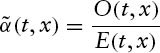
The fundamental quantity we model in this chapter is an intensity α of a particular event that depends on time and some other covariate x. The event may be a single type of event (such as “default”) or it may be an aggregation of several types of events (such as an “upgrade”). If we denote the next occurrence of the event as τ, the intensity provides a local expression for the probability of the event in the sense that the conditional probability P_x,t exists, given that an event can happen at time t (if we consider upgrades, then the particular firm under consideration is actually observed at time t) and that the covariate is around x. Heuristically, we have

A more formal definition of α is based on counting process theory and the concept of stochastic intensities; see Andersen et al. (1993) and Nielsen and Linton (1995). For the purpose of this chapter the definition above is sufficient.

We are interested in considering duration effects, and while it is possible to see some effect on the bivariate graphs, we will study mainly the effects in one dimension. The procedure we use is the following:

• Obtain a non-parametric estimator for the bivariate intensity by smoothing exposures and occurrences separately.
• Construct univariate intensity estimators through “marginal integration”—a technique described below.
• Obtain pointwise confidence sets for the univariate intensities by bootstrapping the bivariate estimator and for each simulation integrating marginally.

We will now describe each procedure in turn and at each step illustrate the technique graphically on a particular rating class.

3. ESTIMATING TRANSITION INTENSITIES IN TWO DIMENSIONS

Our first goal is to estimate the bivariate function α. We can obtain a preliminary estimator for the intensity α(t, x) for a given time t and duration x as follows: Assume that the event we are interested in is “downgrade.” First, count the total number of firms E(t, x) whose covariates were in a small interval around x and t. Among these firms, count the number O(t, x) of firms that were downgraded. A natural estimator for the intensity is then the occurrence/exposure ratio

This analysis is performed on a “grid” of values of x and t.

Even if our original data set is large, we are left with many “cells” in our grid with no occurrences, or, even worse, with no exposures. This is because we have a two-dimensional set of covariates, calendar time and duration, and because we further stratify the data according to the direction of the previous rating move. Whereas most previous studies such as Blume et al. (1998) and Nickell et al. (2000) analyze the old system with eight rating classes, we look at the rating classes with modifiers as well. This decreases exposure, but actually increases occurrences since many moves take place within the finer categories. All in all, this leaves us with many cells in our grid with no information. The purpose of smoothing is to compensate for this thinness by using information from “neighbor” cells in the grid. Smoothing implicitly assumes that the underlying intensity varies smoothly with the covariates, but makes no other assumptions on the functional form. While non-parametric intensity techniques have been widely accepted in actuarial science and biostatistics for years—see Nielsen (1998) and Andersen et al. (1993) for further literature—these methods are still not used much in finance.

We can compute the raw occurrence exposure ratios as above for every considered combination of x and t in our grid and subsequently smooth the intensity function using a two-dimensional smoothing procedure. This would correspond to the internal type of regression estimators; see Jones et al. (1994). However, the external intensity estimator used in this chapter applies smoothing to occurrence and exposure separately. The main reason is that there is evidence from the one-dimensional case that the “external” type of estimator is more robust to volatile exposure patterns than the “internal” estimator; see Nielsen and Tanggaard (2001), who compare the “internal” estimator of Ramlau-Hansen (1983) with the external type similar to the one used in this chapter. Since we do experience volatile exposure patterns, the external smoothing approach described above, therefore seems appropriate for our study.¹

The exact smoothing procedure adapted to our data is defined as follows: We have a grid of N = 50 points in the x-direction and T = 190 points in the t-direction. We compute the smoothed two-dimensional intensity estimator as the ratio

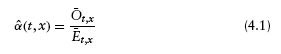
Where the numerator and denominator, the smoothed versions of the “raw” occurrences and exposures, are defined as

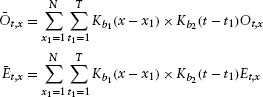
where we have used the so-called Epanechnikov kernel functions

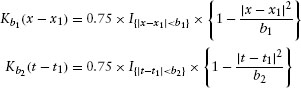
The Epanechnikov kernel function adds more weight to observations close to the point of interest than, for example, a uniform kernel, and less or no weight to points far from the point of interest. The bandwidths essentially determine how far from a grid point (t, x) the occurrences and exposures in other grid points should affect the intensity estimates at (t, x). In this chapter, we choose the grid size and select the bandwidths b₁ b₂ by visual inspection, trying to increase the bandwidth if the graphs appeared too ragged, and to decrease it if there were signs of over smoothing. We used a (common) bandwidth of b₁ = b₂ = 25. This allowed us to smooth out most local changes and capture the long-term trends in data.²

It is illustrative to go through an example of a kernel smoothing step by step. Consider throughout this chapter the class Baa1. In Figure 4.1 we see a graphical representation of the total number of exposures of firms in our data set as a function of time and duration. We show both the raw counts and the smoothed version of these counts. Figure 4.2 shows downgrade activity among the same firms and for the same grid definition as for the exposures. Again, both the raw counts and the smoothed versions are displayed. We see very erratic patterns for the raw counts that are hard to interpret. Naturally, for the downgrade activity, there are many zeros, since for a small handful of firms that typically occupy a particular grid point, a transition is rare.

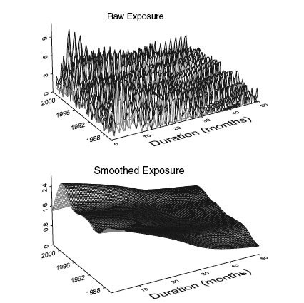
FIGURE 4.1 A graphical illustration of the “exposure” matrix E(t,x), that is, the number of firms “exposed” to making a transition as a function of time and duration, and its smoothed version. The rating class is Baa1. The exposures are divided into “buckets” covering 30-day periods in both duration and calendar time. Hence, an exposure of n at a given grid point (t, x) tells us that at the beginning of a 30-day period starting at date t there were n firms that had been in the state between 30(x – 1) and 30x days. Firms that leave the class are distributed between their old exposure class and their new exposure class.

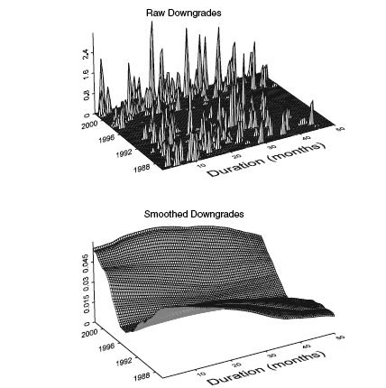
FIGURE 4.2 A graphical illustration of the raw occurrence matrix and its smoothed version for the event downgrade from Baa1 as a function of time and duration. The definitions are the same as in Figure 4.1.

From the smoothed exposure matrix and the smoothed occurrence matrix we are in a position to obtain a bivariate intensity estimate for downgrades. The result is shown in Figure 4.3. Note that this technique maintains the impression of continuous data. In most other studies with sparse data, one has to group data to obtain reasonable statistical results. We do not have to subgroup data in a fixed number of groups when we use the smoothing technique described above.

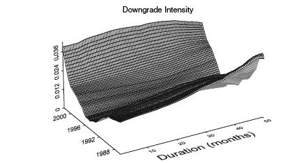
FIGURE 4.3 The smoothed downgrade intensity as a function of time and duration obtained by dividing the smoothed downgrade matrix by the smoothed exposure matrix. The rating category is Baa 1.

4. ONE-DIMENSIONAL HAZARDS AND MARGINAL INTEGRATION

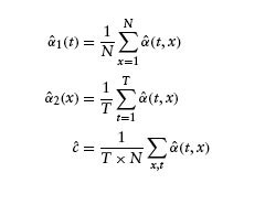
The two-dimensional intensity estimator is a good starting point for our analysis. However, we will often prefer a simpler structure where we can interpret the marginal effect of each explanatory variable. We are primarily interested in the marginal effect of duration (time since last transition), but to make sure we can trust our conclusions we also take into account the effect of different calendar times. Let α(t,x) be the two-dimensional true intensity. Consider the following models:

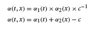
The first model is a multiplicative model. The second model is additive. In both models we can estimate α₁(t) and α₂(x) by marginal integration. (See Linton and Nielsen (1995) for the simple regression analogue and Linton et al. (2003) for a mathematical analysis of the more complicated intensity estimators considered in this paper.) For our data set, the estimators can be written as

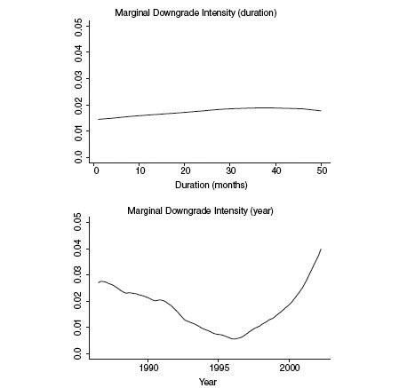
FIGURE 4.4 The marginally integrated upgrade and downgrade intensities as a function of duration in current state (top graph) and calendar time (bottom graph). The rating class is Baa1 and we consider here only the firms that are downgraded into this class.

Note that estimators are the same in the multiplicative and the additive model. So we add more structure to the model by using marginal integration, and we obtain more directly interpretable estimators. Figure 4.4 shows the marginally integrated downgrade intensity with respect to duration and calendar time, respectively, obtained from the smoothed downgrade intensity presented in Figure 4.3. It is interesting to note the strong cyclical behavior of the downgrade intensity component depending on calendar time, whereas the duration effect is very stable, at least for our base case Baa1. The fact that the cyclical behavior is so pronounced is a strong reason to specify a two-dimensional mode before studying the effects of duration. However, as we will see below, we need to be careful in interpreting the graph, since we will see that the Baa1-rated firms actually display a significant heterogeneity with respect to the previous rating move, which needs to be accounted for.

5. CONFIDENCE INTERVALS

Our particular implementation of the bootstrap method is based on the following four steps:

• From the observed occurrence O_t,x and exposure E_t,x we calculate the estimator of α(t,x) using the techniques from Section 3.
• We then simulate n new sets of occurrences. Each observation point in the occurrence matrix is simulated as follows:

  

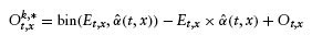
  where the first two terms give us the difference between the simulated and the expected number of transitions, and the last term corrects the overall level of the simulated occurrence matrix.

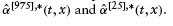
• Third, for each new simulated occurrence matrix O_t,x^k,* a new estimator is calculated based on this new occurrence matrix and the original exposure E_t,x. We store the k = 1,…, 1000. For a given duration x and year t, all are ordered as

• The upper 97.5% and lower 2.5% pointwise confidence interval can now be calculated as

It is possible to construct confidence intervals for both the two-dimensional estimator itself and for smooth functionals of it. Fledelius et al. (2004) provide a general framework for bootstrapping pointwise confidence intervals and give a heuristic argument for why bootstrapping works. In this chapter, we only construct confidence intervals for our marginally integrated intensity estimator for which the asymptotic theory was established in Linton et al. (2003).

6. TRANSITIONS: DEPENDENCE ON PREVIOUS MOVE AND DURATION

We now use the procedure outlined above to investigate some key hypotheses on rating behavior. Our main concern is the influence of previous rating moves on the downgrade and upgrade intensity from the current state. While the stratification according to the previous move is clearly important in itself, the duration effect adds an interesting perspective because it allows us to study for how long the stratification remains important. We also show the marginally integrated upgrade and downgrade intensities over calendar time and finally show that the multiplicative model lying behind this marginal integration seems to describe data well.

While it is possible in principle to investigate the issues for all rating classes, we have decided to focus on one class, Baa1, for the graphs presented here. This class has a fairly large number of observations. When too few observations are present, we must use very large bandwidths, and we therefore obtain “flat” intensity estimates. The other classes we investigated were A1, Baa2, and Ba1, but showing graphs for all of these would be excessive.

We began by stratifying the exposures according to the direction of the previous rating move. This means that the exposure matrix E(t, x) defined above for each rating category is divided into three groups: Those whose previous move was an upgrade, those whose previous move was a downgrade, and those for which there is no information, typically because the current rating class is the first recorded.

In Figure 4.5 we see the result for the rating category Baa1. The pattern displayed here is typical of the classes we investigated. The potentially significant effect we are searching for is in the classification between previous upgrade and previous downgrade. When the event is upgrade, a previous downgrade and no information on the previous move have similar intensities, and when the event is downgrade, a previous upgrade and no information are similar. We found this to be true for the other categories as well.

We therefore focus on the difference in the estimated intensities depending on whether the previous move was an upgrade or a downgrade. Our goal is to check whether and for which durations there are significant differences. To analyze this “rating drift” issue, we present intensity estimates as a function of duration in a state with confidence bounds. Figure 4.6 shows the downgrade and upgrade from intensities from Baa1, respectively, as a function of how long the company has been in class Baa1 and stratified according to the previous move. The intensities are shown with bootstrapped pointwise confidence intervals.

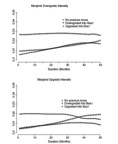
FIGURE 4.5 Downgrade and upgrade intensities from Baa1 stratified according to direction of the previous move with no information on the previous move as a separate category.

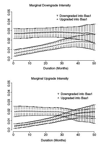
FIGURE 4.6 Downgrade and upgrade intensities with confidence bounds from Baa1 as a function of duration, stratified by the previous move

Clearly, the most pronounced effect is seen for downgrades from Baa1, where for most durations there is a significantly higher intensity of downgrades for the firms that were downgraded into Baa1 than for those that were upgraded into Baa1. The downgrade intensity for companies that were downgraded into Baa1 is fairly constant for the first 25–30 periods; after that we see a decrease in the level. The downgrade intensity for companies upgraded into Baa1 starts out at low values, and we see an increase in intensity with length of stay. If a company is upgraded into Baa1, we see very little downgrade activity in the first l0–20 periods. The gap between the intensities disappears after 25–30 periods. In summary, the previous rating change direction gives extra information for companies that have stayed in Baa1 for less than 30 periods of 30 days, that is, somewhere between 2 and 3 years.

The upgrade intensities display a pattern similar to that for downgrades in the sense that the data for the previous transition contains important information for around 25 to 30 periods. This is evident from the low upgrade intensity in the first 25 periods for companies downgraded into Baa1. Both cases seem to support the observation that rating reversals are rare in Moody's rating history. They also show that the memory is approximately 25 to 30 periods, equivalent to 2–2.5 years. We also investigated other classes and the conclusions were similar. It is clear that the largest effect of stratification is for the cases where the event considered is a downgrade. Here, the intensity is significantly lower when the previous move was an upgrade. In most cases, but not for Ba1, the downgrade intensity is relatively constant as a function of duration in the state when the previous move was a downgrade. This is evidence that the difference in intensity is not so much due to firms that are given a sequence of downgrades “one at a time” but rather a “reversal aversion effect” that a firm is unlikely to be upgraded following a downgrade. The effect seems to vanish after between 20–30 periods in a state.

We also find that the upgrade intensities seem to be higher when the previous move was an upgrade than when it was a downgrade. The effect is not as pronounced as for downgrades, but it is still significant. Again, the history seems more consistent with rating reversal aversion than with rating momentum in that the intensity for upgrade on the condition that the previous move was an upgrade is relatively constant across duration.

7. MULTIPLICATIVE INTENSITIES

In our study, we have noticed a clear intensity variation with calendar time, and we therefore cannot investigate the effect of duration through a one-dimensional analysis. We have to consider the two-dimensional intensity case. However, the one-dimensional estimates that we obtain through marginal integration from the smoothed two-dimensional estimates can be interpreted properly only if the intensity model can reasonably be thought of as multiplicative or additive, as explained in Section 4. We therefore implement a visual inspection of the multiplicative and the additive intensity models and compute a measure for squared error to see which one fits the data best. The visual inspection consists of comparing the two-dimensional estimator obtained by adding or multiplying the two marginally integrated intensities with the smoothed but unrestricted two-dimensional estimator. In Figure 4.7 we show the smoothed but unrestricted bivariate downgrade intensity for firms that were downgraded into Baa1. If we perform a marginal integration as explained in Section 4 to obtain the downgrade intensity as a function of both duration and calendar time, we obtain the results shown in Figure 4.8 (where we also show the marginally integrated upgrade intensities for comparison). From the marginally integrated intensities we can now show the bivariate intensity, assuming a multiplicative and an additive structure, respectively. The resulting bivariate intensities are shown in Figure 4.9. A visual inspection confirms that the multiplicative intensity is closer to the unrestricted intensity estimate. Certainly, the difference between these graphs and the unrestricted estimators in Figure 4.7 does not lead us to reject the assumption of a multiplicative structure, even if the multiplicative structure is smoother and does not capture all of the features of the unrestricted estimator.

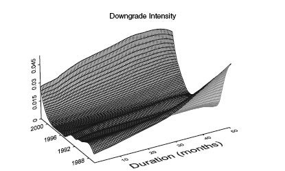
FIGURE 4.7 The bivariate intensity estimator for the class Baa1 when the previous move was a downgrade.

We would also prefer the multiplicative structure to the additive structure based on a computation of squared errors and for reasons of interpretation. The multiplicative model is

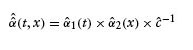
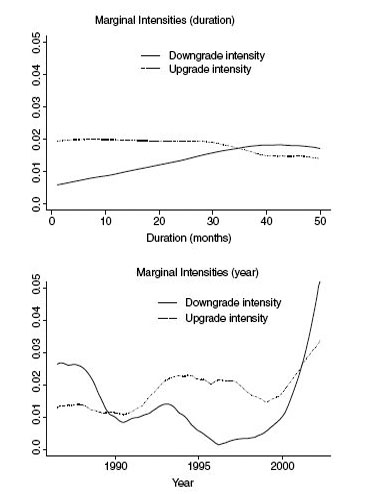
FIGURE 4.8 The marginally integrated upgrade and downgrade intensities as functions of duration in current state (top graph) and calendar time (bottom graph). The rating class is Baa1 and we consider here only the firms that are downgraded into this class.

Let denote the corresponding intensity estimator in the additive model. We calculated the sums of squared errors (SSEs) for defined as

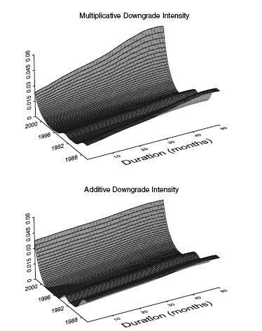
FIGURE 4.9 The bivariate intensity estimator for firms downgraded into class Baa1 assuming a multiplicative intensity structure (top graph) and an additive intensity structure (bottom graph). The multiplicative (additive) structure defines the intensity as the product (sum) of the marginally integrated intensities.

and

The event considered was a downgrade from Baa1, and to avoid the problems with heterogeneity within this class, we chose only the firms that were downgraded into Baa1. We found an SSE in the multiplicative model of 0.048 and an SSE in the additive model of 0.103. The SSE calculation, therefore, supports selecting the multiplicative model for downgrades.

8. CONCLUDING REMARKS

This chapter applies non-parametric smoothing techniques to the study of rating transitions in Moody's corporate default database. The techniques give a powerful way of visualizing data. We illustrate their use with a detailed study of both duration dependence of transitions and the direction of a previous rating move. The patterns we see for Baa1 (and for the other classes we investigated but do not display here) are consistent with a policy of “rating reversal aversion” in which the ratings through a period of 2–3 years show a reduced tendency of moving in a direction opposite to the direction in which they were moved into the current state. It is also consistent with Moody's stated objectives, as formulated in Cantor (2001), of changing ratings only when a reversal is unlikely to take place in the foreseeable future. This pattern is significant in both directions; that is, downgrades are less likely for firms that were upgraded into the state than for firms downgraded into the state, and the pattern is reversed when studying upgrades. The effect of stratification is, however, most pronounced for downgrade activity.

One may also attribute this observed pattern to an effect caused by multinotch downgrades being carried out one notch at a time for some firms despite the fact that they have in reality experienced a credit quality decline. If this were the pattern, we should see significant duration effects on downgrade activity as a function of duration but we found a clear pattern of this only for the rating class Baa2. We show clear calendar time effects in our data set, as demonstrated, in Figure 4.8, and this is consistent with, for example, Nickell et al. (2000). We condition out those effects through the marginal integration procedure. This procedure works well under either an additive or a multiplicative intensity structure and we find support for the treatment of the model as a multiplicative model, consistent with the semiparametric Cox regression studied, for example, in Lando and Skødeberg (2002). About the time of completion of this work, the study of Hamilton and Cantor (2004) emerged, which as earlier mentioned, studies the role of outlooks and watch lists. This also lends support to the non Markovian pattern found here but the precise role of the outlooks in our setting awaits further analysis.

ACKNOWLEDGMENTS

We are grateful to Moody's for providing the data and in particular to Richard Cantor and Roger Stein for their assistance. Helpful comments from an anonymous referee are also gratefully acknowledged. All errors and opinions are, of course, our own. Lando acknowledges partial support by the Danish Natural and Social Science Research Councils.

NOTES

1. To our knowledge, the asymptotic theory is also only fully understood in the external case.

2. We could have chosen to work with quantitative criteria for bandwidth selection. There is extensive literature on bandwidth selection with the simple kernel density estimator as the primary object of interest. In our intensity case, the analogue to the most widely used bandwidth selection procedure, cross-validation, was introduced in Nielsen and Linton (1995) and Fledelius et al. (2004). Automatic bandwidth selection turns out to be extremely complicated in practice and no one method has yet obtained universal acceptance; see Wand and Jones (1995). For example, the simplest and most widely used method, cross-validation, is well known to be a bad bandwidth selector for many data sets; see Wand and Jones (1995).

REFERENCES

Altman, E. and Kao, D. (1992a). Corporate Bond Rating Drift: An Examination of Credit Quality Rating Changes over Time. IFCA, Charlottesville: The Research Foundation of the Institute of Chartered Financial Analysts.

Altman, E. and Kao, D. (1992b). “The Implications of Corporate Bond Rating Drift.” Financial Analysts Journal 3, 64–75.

Altman, E. and Kao, D. (1992c). Rating drift in high yield bonds. The Journal of Fixed Income 1, 15–20.

Andersen, P., Borgan, Ø., Gill, R. and Keiding, N. (1993). Statistical Models Based on Counting Processes. New York: Springer.

Bangia, A., Diebold, F., Kronimus, A., Schagen, C. and Schuermann, T. (2002). “Ratings Migration and the Business Cycle, with Applications to Credit Portfolio Stress Testing.” Journal of Banking and Finance 26(2–3), 445–474.

Blume, M., Lim, F. and MacKinlay, A. (1998). “The Declining Credit Quality of US Corporate Debt: Myth or Reality.” Journal of Finance 53(4), 1389–1413.

Cantor, R. (2001). “Moody's Investors Service Response to the Consultative Paper Issued by the Basel Committee on Bank Supervision a New Capital Adequacy Framework.” Journal of Banking and Finance 25, 171–185.

Carty, L. (1997). Moody's Rating Migration and Credit Quality Correlation, 1920–1996. Special Comment, Moody's Investors Service, New York.

Fan, J. and Gijbels, I. (1996). Local Polynomial and Its Applications. London: Chapman and Hall.

Fledelius, P., Guillen, M., Nielsen, J. and Vogelius, M. (2004). “Two-dimensional Hazard Estimation for Longevity Analyses.” Scandinavian Actuarial Journal 2, 133–156.

Fusaro, R., Nielsen, J. P. and Scheike, T. (1993). “Marker Dependent Hazard Estimation. An Application to Aids.” Statistics in Medicine 12, 843–865.

Hamilton, D. and Cantor, R. (2004). Rating Transitions and Defaults Conditional on Watchlist. Outlook and Rating History. Special Comment, Moody's Investors Service, New York.

Jones, M. C., Davies, D. and Park, B. U. (1994). “Versions of Kernel-type Regression Estimators.” Journal of the American Statistical Association 89, 825–832.

Kavvathas, D. (2000). “Estimating Credit Rating Transition Probabilities for Corporate Bonds.” Working Paper, Department of Economics, University of Chicago.

Lando, D. and Skødeberg, T. (2002). “Analyzing Rating Transitions and Rating Drift with Continuous Observations.” The Journal of Banking and Finance 26, 423–444.

Linton, O. and Nielsen, J. P. (1995). “A Kernel Method of Estimating Structure Nonparametric Regression Based on Marginal Integration.” Biometrika 82, 93–100.

Linton, O., Nielsen, J. and de Geer, S. V. (2003). “Estimating Multiplicative and Additive Hazard Functions by Kernel Methods.” Annals of Statistics 31, 464–492.

Löffler, G. (2003). “Avoiding the Rating Bounce: Why Rating Agencies Are Slow to React to New Information.” Working Paper, Goethe Universität, Frankfurt.

Löffler, G. (2004). “An Anatomy of Rating Through the Cycle.” Journal of Banking and Finance 28, 695–720.

Lucas, D. and Lonski, J. (1992). “Changes in Corporate Credit Quality 1970–1990.” The Journal of Fixed Income 1, 7–14.

Nickell, P., Perraudin, W. and Varotto, S. (2000). “Stability of Ratings Transitions.” Journal of Banking and Finance 24(1–2), 203–227.

Nielsen, J. P. (1998). “Marker Dependent Kernel Hazard Estimation from Local Linear Estimation.” Scandinavian Actuarial Journal 2, 113–124.

Nielsen, J. and Linton, O. (1995). “Kernel Estimation in a Nonparametric Marker Dependent Hazard Model. ” Annals of Statistics 23, 1735–1748.

Nielsen, J. P. and Tanggaard, C. (2001). “Boundary and Bias Correction in Kernel Hazard Estimation.” Scandinavian Journal of Statistics 28, 675–698.

Ramlau-Hansen, H. (1983). “Smoothing Counting Processes by Means of Kernel Functions.” Annals of Statistics 11, 453–466.

Sobehart, J. and Stein, R. (2000). “Moody's Public Firm Risk Model: A Hybrid Approach to Modeling Short Term Default Risk.” Moody's Investors Service. Global Credit Research.

Wand, M. P. and Jones, M. C. (1995). Kernel Smoothing. London: Chapman and Hall.

Keywords: Credit ratings; transition probabilities; non-Markov effects; non-parametric analysis