


Storage area network guidelines
The storage area network (SAN) is one of the most important aspects when implementing and configuring an IBM Spectrum Virtualize. Because of their unique behavior and the interaction with other storage, specific SAN design and zoning recommendations differ from classic storage practices.
This chapter provides guidance to connect IBM Spectrum Virtualize in a SAN to achieve a stable, redundant, resilient, scalable, and performance-likely environment. Although this chapter does not describe how to design and build a flawless SAN from the beginning, you can consider the principles that are presented here when building your SAN.
This chapter includes the following sections:
2.1 SAN topology general guidelines
The SAN topology requirements for IBM SAN Volume Controller do not differ too much from any other SAN. Remember that a well-sized and designed SAN enables you to build a redundant and failure-proof environment, and minimizing performance issues and bottlenecks. Therefore, before installing any of the products covered by this book, ensure that your environment follows an actual SAN design and architecture, with vendor-recommended SAN devices and code levels.
For more information about SAN design and preferred practices, see SAN Fabric Administration Best Practices Guide.
A topology is described in terms of how the switches are interconnected. There are several different SAN topologies, such as core-edge, edge-core-edge, or full mesh. Each topology has its utility, scalability, and also its cost, so one topology will be a better fit for some SAN demands than others. Independent of the environment demands, there are a few best practices that must be followed to keep your SAN working correctly, performing well, redundant, and resilient.
2.1.1 SAN performance and scalability
Regardless of the storage and the environment, planning and sizing of the SAN makes a difference when growing your environment and when troubleshooting problems.
Because most SAN installations continue to grow over the years, the main SAN industry-lead companies design their products in a way to support a certain growth. Keep in mind that your SAN must be designed to accommodate both short-term and medium-term growth.
From the performance standpoint, the following topics must be evaluated and considered:
•Host-to-storage fan-in fan-out ratios
•Host to inter-switch link (ISL) oversubscription ratio
•Edge switch to core switch oversubscription ratio
•Storage to ISL oversubscription ratio
•Size of the trunks
•Monitor for slow drain device issues
From the scalability standpoint, ensure that your SAN will support the new storage and host traffic. Make sure that the chosen topology will also support a growth not only in performance, but also in port density.
If new ports need to be added to the SAN, you might need to drastically modify the SAN to accommodate a larger-than-expected number of hosts or storage. Sometimes these changes increase the number of hops on the SAN, and so cause performance and ISL congestion issues. For more information, see 2.1.2, “ISL considerations” on page 23.
Consider the use of SAN director-class switches. They reduce the number of switches in a SAN and provide the best scalability available. Most of the SAN equipment vendors provide high port density switching devices. With MDS 9718 Multilayer Director, Cisco offers the industry’s highest port density single chassis with up to 768 16/32 Gb ports. The Brocade UltraScale Inter-Chassis Links (ICL) technology enables you to create multichassis configurations with up to 4608 16/32 Gb ports.
Therefore, if possible, plan for the maximum size configuration that you expect your IBM SAN Volume Controller (SAN Volume Controller or IBM SAN Volume Controller) installation to reach. Planning for the maximum size does not mean that you must purchase all of the SAN hardware initially. It requires you to design only the SAN to reach the expected maximum size.
2.1.2 ISL considerations
ISLs are responsible for interconnecting the SAN switches, creating SAN flexibility and scalability. For this reason, they can be considered as the core of a SAN topology. Consequently, they are sometimes the main cause of issues that can affect a SAN. For this reason it is important to take extra caution when planning and sizing the ISL in your SAN.
Regardless of your SAN size, topology, or the size of your SAN Volume Controller installation, consider the following practices to your SAN Inter-switch link design:
•Beware of the ISL oversubscription ratio
The standard recommendation is up to 7:1 (seven hosts using a single ISL). However, it can vary according to your SAN behavior. Most successful SAN designs are planned with an oversubscription ratio of 7:1 and some extra ports are reserved to support a 3:1 ratio. However, high-performance SANs start at a 3:1 ratio.
Exceeding the standard 7:1 oversubscription ratio requires you to implement fabric bandwidth threshold alerts. If your ISLs exceed 70%, schedule fabric changes to distribute the load further.
•Avoid unnecessary ISL traffic
Connect all SAN Volume Controller node ports in a clustered system to the same SAN switches or Directors as all of the storage devices with which the clustered system of SAN Volume Controller is expected to communicate. Conversely, storage traffic and internode traffic must never cross an ISL (except during migration scenarios).
Keep high-bandwidth use servers and I/O Intensive application on the same SAN switches as the SAN Volume Controller host ports. Placing these servers on a separate switch can cause unexpected ISL congestion problems. Also, placing a high-bandwidth server on an edge switch wastes ISL capacity.
•Properly size the ISLs on your SAN. They must have adequate bandwidth and buffer credits to avoid traffic or frames congestion. A congested inter-switch link can affect the overall fabric performance.
•Always deploy redundant ISLs on your SAN. Using an extra ISL avoids congestion if an ISL fails because of certain issues, such as a SAN switch line card or port blade failure.
•Use the link aggregation features, such as Brocade Trunking or Cisco Port Channel, to obtain better performance and resiliency.
•Avoid exceeding two hops between the SAN Volume Controller and the hosts. More than two hops are supported. However, when ISLs are not sized properly, more than two hops can lead to ISL performance issues and buffer credit starvation (SAN congestion).
When sizing over two hops, consider that all of the ISLs that go to the switch where the SAN Volume Controller is connected also handle the traffic that is coming from the switches on the edges, as shown in Figure 2-1.
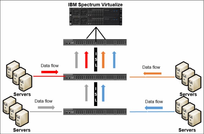
Figure 2-1 ISL data flow
Consider the following points:
•If possible, use SAN directors to avoid many ISL connections. Problems that are related to oversubscription or congestion are much less likely to occur within SAN director fabrics.
•When interconnecting SAN directors through ISL, spread the ISL cables across different directors blades. In a situation where an entire blade fails, the ISL will still be redundant through the links connected to other blades.
•Plan for the peak load, not for the average load.
2.2 SAN topology-specific guidelines
Some preferred practices (see 2.1, “SAN topology general guidelines” on page 22) apply to all SANs. However, specific preferred practices requirements exist for each available SAN topology. In this section, we discuss the differences between the types of topology and highlight the specific considerations for each.
This section covers the following topologies:
•Single switch fabric
•Core-edge fabric
•Edge-core-edge
•Full mesh
2.2.1 Single switch SAN Volume Controller SANs
The most basic SAN Volume Controller topology consists of a single switch per SAN fabric. This switch can range from a 24-port 1U switch for a small installation of a few hosts and storage devices, to a director with hundreds of ports. This configuration is a low-cost design solution that has the advantage of simplicity and is a sufficient architecture for small-to-medium SAN Volume Controller installations.
One of the advantages of a single switch SAN is that no hop exists when all servers and storages are connected to the same switches.
|
Note: To meet redundancy and resiliency requirements, a single switch solution needs at least two SAN switches or SAN directors (one per different fabric).
|
The preferred practice is to use a multislot director-class single switch over setting up a core-edge fabric that is made up solely of lower-end switches, as described in 2.1.1, “SAN performance and scalability” on page 22.
The single switch topology, as shown in Figure 2-2, has only two switches; therefore, the IBM SAN Volume Controller ports must be equally distributed on both fabrics.
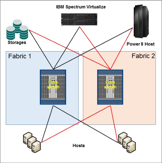
Figure 2-2 Single-switch SAN
|
Note: To correctly size your network, always calculate the short-term and mid-term growth to avoid lack of ports. On this topology, the limit of ports is based on the switch size. If other switches are added to the network, the topology type is changed automatically.
|
2.2.2 Basic core-edge topology
The core-edge topology (as shown in Figure 2-3) is easily recognized by most SAN architects. This topology consists of a switch in the center (usually, a director-class switch), which is surrounded by other switches. The core switch contains all SAN Volume Controller ports, storage ports, and high-bandwidth hosts. It is connected by using ISLs to the edge switches. The edge switches can be of any size from 24 port switches up to multi-slot directors.
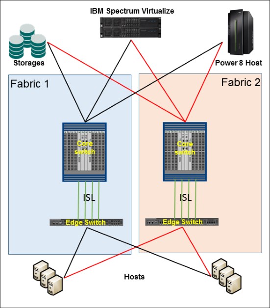
Figure 2-3 Core-edge topology
When the SAN Volume Controller nodes and servers are connected to different switches, the hop count for this topology is one.
|
Note: This topology is commonly used to easily growth your SAN network by adding edge switches to the core. Consider the ISL ratio and use of physical ports from the core switch when adding edge switches to your network.
|
2.2.3 Edge-core-edge topology
Edge-core-edge is the most scalable topology, it is used for installations where a core-edge fabric made up of multislot director-class SAN switches is insufficient. This design is useful for large, multiclustered system installations. Similar to a regular core-edge, the edge switches can be of any size, and multiple ISLs must be installed per switch.
Figure 2-4 shows an edge-core-edge topology with two different edges, one of which is exclusive for the storage, IBM SAN Volume Controller, and high-bandwidth servers. The other pair is exclusively for servers.

Figure 2-4 Edge-core-edge topology
Performance can be slightly affected if the number of hops increase, depending on the total number of switches and the distance between host and IBM SAN Volume Controller.
Edge-core-edge fabrics allow better isolation between tiers. For more information, see 2.2.6, “Device placement” on page 29.
2.2.4 Full mesh topology
In a full mesh topology, all switches are interconnected to all other switches on the same fabric. Therefore, the server and storage placement is not a concern after the number of hops is no more than one hop. A full mesh topology is shown in Figure 2-5.
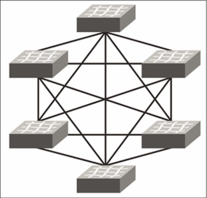
Figure 2-5 Full mesh topology
|
Note: Each ISL uses one physical port. Depending on the total number of ports each switch has and the total number of switches, this topology uses several ports from your infrastructure to be set up.
|
2.2.5 IBM Spectrum Virtualize as a multi SAN device
IBM SAN Volume Controller nodes now have a maximum of 16 ports. In addition to the increased throughput capacity, this number of ports enables new possibilities and allows different kinds of topologies and migration scenarios.
One of these topologies is the use of a IBM SAN Volume Controller as a multi SAN device between two isolated SANs. This configuration is useful for storage migration or sharing resources between SAN environments without merging them.
To use an external storage with IBM SAN Volume Controller, this external storage must be attached to IBM SAN Volume Controller through the zoning configuration and set up as virtualized storage. This feature can be used for storage migration and decommission processes and to speed up host migration. In some cases, based on the external storage configuration, virtualizing external storage with IBM SAN Volume Controller can increase performance based on the cache capacity and processing.
Figure 2-6 shows an example of an IBM Spectrum Virtualize as a multi SAN device.
Figure 2-6 IBM Spectrum Virtualize as SAN bridge
Notice in Figure 2-6 that both SANs (blue and red) are isolated. When connected to both SAN networks, IBM SAN Volume Controller can allocate storage to hosts on both SAN networks. It also is possible to virtualize storages from each SAN networks. In this way, you can have established storage on the green SAN (SAN 2 in Figure 2-6) that is attached to IBM SAN Volume Controller and provide disks to hosts on the blue network (SAN 1 in Figure 2-6). This configuration is commonly used for migration purposes or in cases where the established storage has a lower performance compared to IBM SAN Volume Controller.
2.2.6 Device placement
With the growth of virtualization, it is not usual to experience frame congestion on the fabric. Device placement seeks to balance the traffic across the fabric to ensure that the traffic is flowing in a specific way to avoid congestion and performance issues. The ways to balance the traffic consist of isolating traffic by using zoning, virtual switches, or traffic isolation zoning.
Keeping the traffic local to the fabric is a strategy to minimize the traffic between switches (and ISLs) by keeping storages and hosts attached to the same SAN switch, as shown in Figure 2-7.

Figure 2-7 Storage and hosts attached to the same SAN switch
This solution can fit well in small- and medium-sized SANs. However, it is not as scalable as other topologies available. The most scalable SAN topology is the edge-core-edge, as described in 2.2, “SAN topology-specific guidelines” on page 24.
In addition to scalability, this topology provides different resources to isolate the traffic and reduce possible SAN bottlenecks. Figure 2-8 shows an example of traffic segregation on the SAN by using edge-core-edge topology.

Figure 2-8 Edge-core-edge segregation
Even when sharing core switches, it is possible to use virtual switches (see “SAN partitioning” on page 31) to isolate one tier from the other. This configuration helps avoid traffic congestion that is caused by slow drain devices that are connected to the backup tier switch.
SAN partitioning
SAN partitioning is a hardware-level feature that allows SAN switches to share hardware resources by partitioning its hardware into different and isolated virtual switches. Both Brocade and Cisco provide SAN partitioning features called, respectively, Virtual Fabric and Virtual SAN (VSAN).
Hardware-level fabric isolation is accomplished through the concept of switch virtualization, which allows you to partition physical switch ports into one or more “virtual switches.” Virtual switches are then connected to form virtual fabrics.
From a device perspective, SAN partitioning is completely transparent and so the same guidelines and practices that apply to physical switches apply also to the virtual ones.
Although the main purposes of SAN partitioning are port consolidation and environment isolation, this feature is also instrumental in the design of a business continuity solution based on IBM Spectrum Virtualize.
For more information about IBM Spectrum Virtualize business continuity solutions, see Chapter 7, “Meeting business continuity requirements” on page 343.
2.3 IBM SAN Volume Controller ports
Port connectivity options were significantly changed in IBM SAN Volume Controller hardware, as listed in Table 2-1.
Table 2-1 IBM SAN Volume Controller connectivity
|
Feature
|
2145-DH8
|
2145-SV1
|
2145-SV2
|
2145-SA2
|
|
Fibre Channel Host Bus Adapter
|
4x Quad 8 Gb
4x Dual 16 Gb
4x Quad 16 Gb
|
4x Quad 16 Gb
|
3x Quad 16/32 Gb (FC-NVMe supported)
|
3x Quad 16/32 Gb (FC-NVMe supported)
|
|
Ethernet I/O
|
4x Quad 10 Gb iSCSI/FCoE
|
4x Quad 10 Gb iSCSI/FCoE
|
1x Dual 25 Gb (available up to 3x 25 Gb)
|
1x Dual 25 Gb (available up to 3x 25 Gb)
|
|
Built in ports
|
4x 1 Gb
|
4x 10 Gb
|
4x 10 Gb
|
4x 10 Gb
|
|
SAS expansion ports
|
4x 12 Gb SAS
|
4x 12 Gb SAS
|
N/A
|
N/A
|
|
Note: Ethernet Adapters support RoCE and iWARP.
|
This new port density expands the connectivity options and provides new ways to connect the IBM SAN Volume Controller to the SAN. This sections describes some preferred practices and use cases that show how to connect a SAN volume controller on the SAN to use this increased capacity.
2.3.1 Slots and ports identification
The IBM SAN Volume Controller can have up to four quad Fibre Channel (FC) host bus adapter (HBA) cards (16 FC ports) per node. Figure 2-9 shows the port location in the rear view of the 2145-SV1 node.

Figure 2-9 SAN Volume Controller 2145-SV1 rear port view
Figure 2-10 shows the port locations for the SV2/SA2 nodes.

Figure 2-10 SV2/SA2 node layout
For maximum redundancy and resiliency, spread the ports across different fabrics. Because the port count varies according to the number of cards that is included in the solution, try to keep the port count equal on each fabric.
2.3.2 Port naming and distribution
In the field, fabric naming conventions vary. However, it is common to find fabrics that are named, for example, PROD_SAN_1 and PROD_SAN_2, or PROD_SAN_A and PROD_SAN_B. This type of naming convention is used to simplify the SAN Volume Controller, after their denomination followed by 1 and 2 or A and B, which specifies that the devices connected to those fabrics contains the redundant paths of the same servers and SAN devices.
To simplify the SAN connection identification and troubleshooting, keep all odd ports on the odd fabrics, or “A” fabrics and the even ports on the even fabric or “B” fabrics, as shown in Figure 2-11.

Figure 2-11 SAN Volume controller model 2145-SV1 port distribution
SAN Volume Controller clusters follow the same arrangement, odd ports to odd or “A” Fabric, and even ports that are attached to even fabrics or “B” fabric.
As a preferred practice, assign specific uses to specific SAN volume controller ports. This technique helps optimize the port utilization by aligning the internal allocation of hardware CPU cores and software I/O threads to those ports.
Figure 2-12 shows the specific port use guidelines for IBM SAN Volume Controller and Spectrum Virtualize products.

Figure 2-12 Port use guidelines for IBM SAN Volume Controller and Spectrum Virtualize products
Because of port availability on IBM SAN Volume Controller clusters, and the increased bandwidth with the 16 Gb ports, it is possible to segregate the port assignment between hosts and storage, thus isolating their traffic.
Host and storage ports have different traffic behavior, so keeping host and storage ports together produces maximum port performance and utilization by benefiting from its full duplex bandwidth. For this reason, sharing host and storage traffic in the same ports is generally the preferred practice.
However, traffic segregation can also provide some benefits in terms of troubleshooting and host zoning management. For example, consider SAN congestion conditions that are the result of a slow draining device. Because of this issue, all slower hosts (that is, hosts with port speeds that are more than 2x less the IBM SAN Volume Controller node port speeds) should be isolated to their own IBM SAN Volume Controller node ports with no other hosts or controllers zoned to these ports where possible.
In this case, segregating the ports simplifies the identification of the device causing the problem. At the same time, it limits the effects of the congestion to the hosts or backend ports only. Furthermore, dedicating ports for host traffic reduces the possible combinations of host zoning and simplifies SAN management. It is advised to implement the port traffic segregation with configurations with a suitable number of ports (that is, 12 ports or more) only.
|
Note: Consider the following points:
•On IBM SAN Volume Controller clusters with 12 ports or more per node, if you use advanced copy services (such as Volume Mirroring, flash copies, or remote copies), it is recommended that you use four ports per node for inter-node communication. The IBM SAN Volume Controller uses the internode ports for all of these functions and the use of these features greatly increases the data rates that are sent across these ports. If you are implementing a new cluster and plan to use any copy services, plan on having 12 ports per cluster node.
•Use port masking to assign specific uses to the SAN Volume Controller ports. For more information, see Chapter 8, “Configuring host systems” on page 353.
|
Buffer credits
SAN Volume Controller ports feature a predefined number of buffer credits. The amount of buffer credits determines the available throughput over distances:
•All 8 Gbps adapters have 41 credits available per port, saturating links at up to 10 km (6.2 miles) at 8 Gbps
•2-port 16 Gbps (DH8 only nodes) adapters have 80 credits available per port, saturating links at up to 10 km (6.2 miles) at 16 Gbps
•4-port 16 Gbps adapters have 40 credits available per port, saturating links at up to 5 km at (3.1 miles)16 Gbps
|
Switch port buffer credit: For stretched cluster and IBM HyperSwap configurations that do not use ISLs for the internode communication, it is advised to set the switch port buffer credits to match the IBM Spectrum Virtualize port.
|
Port designation and CPU cores utilization
The ports assignment or designation recommendation is based on the relationship between a single port to a CPU and core.
Figure 2-13 shows the port to CPU core mapping for a 2145-SV1 node.

Figure 2-13 Port to CPU core mapping for SV1 nodes
Figure 2-14 shows the port to CPU core mapping for SV2 nodes.

Figure 2-14 Port to CPU core mapping for SV2 nodes
|
N_Port ID Virtualization feature: On N_Port ID Virtualization (NPIV)-enabled systems, the port to CPU core assignment for the virtual WWPN is the same as the physical WWPN.
|
Assignment is valid only for SCSI FC connections. FC-NVMe uses a different model. Multiple CPU cores are assigned to ports in round robin fashion.
This assignment is not tied to physical CPU sockets; rather, it is only about distribution of the FC driver workload across cores and this port assignment can change from release versions.
2.4 Zoning
Because of the nature of storage virtualization and cluster scalability, the IBM SAN Volume Controller zoning differs from traditional storage devices. Zoning an IBM SAN Volume Controller cluster into a SAN fabric requires planning and following specific guidelines.
|
Important: Errors that are caused by improper SAN Volume Controller zoning are often difficult to isolate and the steps to fix them can affect the SAN environment. Therefore, create your zoning configuration carefully.
|
The initial configuration for SAN Volume Controller requires the following different zones:
•Internode and intra-cluster zones
•Replication zones (if replication is used)
•Back-end storage to SAN Volume Controller zoning
•Host to SAN Volume Controller zoning
Different guidelines must be followed for each zoning type, as described in 2.4.1, “Types of zoning” on page 36.
|
Note: Although internode and intra-cluster zone is not necessary for non-clustered IBM Storwize family systems, it is generally preferred to use one of these zones.
|
2.4.1 Types of zoning
Modern SAN switches feature two types of zoning: Port zoning, and worldwide port name (WWPN) zoning. The preferred method is to use only WWPN zoning. A common misconception is that WWPN zoning provides poorer security than port zoning, which is not the case. Modern SAN switches enforce the zoning configuration directly in the switch hardware. Also, you can use port binding functions to enforce a WWPN to be connected to a specific SAN switch port.
When switch-port based zoning is used, the ability to allow only specific hosts to connect to an IBM SAN Volume Controller cluster is lost.
Consider an NPV device, such as an Access Gateway that is connected to a fabric. If 14 hosts are attached to that NPV Device, and switch port-based zoning is used to zone the switch port for the NPV device to IBM SAN Volume Controller node ports, all 14 hosts can potentially connect to the IBM SAN Volume Controller cluster, even if the IBM SAN Volume Controller is virtualizing storage for only 4 or 5 of those hosts.
However, the problem is exacerbated when the IBM SAN Volume Controller NPIV feature is used in transitional mode. In this mode, a host can connect to the physical and virtual WWPNs on the cluster. With switch port zoning, this configuration doubles the connection count for each host attached to the IBM SAN Volume Controller cluster. This issue can affect the function of path failover on the hosts by resulting in too many paths, and the IBM SAN Volume Controller Cluster can exceed the maximum host connection count on a large fabric.
If you have the NPIV feature enabled on your IBM SAN Volume Controller, you must use WWPN-based zoning.
|
Zoning types: Avoid the use of a zoning configuration that includes a mix of port and WWPN zoning.
|
A preferred practice for traditional zone design calls for single initiator zoning. That is, a zone can consist of many target devices, but only one initiator because target devices often wait for an initiator device to connect to them, while initiators actively attempt to connect to each device to which they are zoned. The singe initiator approach removes the possibility of a misbehaving initiator affecting other initiators.
The drawback to single initiator zoning is that on a large SAN that features many zones, the SAN administrator’s job can be more difficult, and the number of zones on a large SAN can exceed the zone database size limits.
Cisco and Brocade developed features that can reduce the number of zones by allowing the SAN administrator to control which devices in a zone can communicate with other devices in the zone. The features are called Cisco Smart Zoning and Brocade Peer Zoning, which are supported with IBM Spectrum Virtualize systems.
A brief overview of these features is provided next.
|
Note: Brocade Traffic Isolation (TI) zoning is deprecated in FOS v9.0. You can still use TI zoning if you have existing zones, but you must keep at least one switch running a pre-9.0 version of FOS in the fabric to be able to make changes to the TI zones.
|
Cisco Smart Zoning
Cisco Smart Zoning is a feature that, when enabled, restricts the initiators in a zone to communicate only with target devices in the same zone. For our cluster example, this feature allows a SAN administrator to zone all of the host ports for a VMware cluster in the same zone with the storage ports to which all of the hosts need access. Smart Zoning configures the access control lists in the fabric routing table to allow only the initiator (host) ports to communicate with target ports.
For more information about Smart Zoning, see this web page.
For more information about implementation, see this IBM Support web page.
Brocade Peer Zoning
Brocade Peer Zoning is a feature that provides a similar functionality of restricting what devices can see other devices within the same zone. However, Peer Zoning is implemented such that some devices in the zone are designated as principal devices. The non-principal devices can only communicate with the principal device, not with each other. As with Cisco, the communication is enforced in the fabric routing table.
For more information, see Peer Zoning in Modernizing Your IT Infrastructure with IBM b-type Gen 6 Storage Networking and IBM Spectrum Storage Products, SG24-8415.
|
Note: Use Smart and Peer zoning for the host zoning only. Use traditional zoning for intracluster, back-end, and intercluster zoning.
|
Simple zone for small environments
As an option for small environments, IBM Spectrum Virtualize-based systems support a simple set of zoning rules that enable a small set of host zones to be created for different environments.
For systems with fewer than 64 hosts that are attached, zones that contain host HBAs must contain no more than 40 initiators, including the ports that acts as initiators, such as the IBM Spectrum Virtualize based system ports that are target + initiator.
Therefore, a valid zone can be 32 host ports plus 8 IBM Spectrum Virtualize based system ports. Include only one port from each node in the I/O groups that are associated with this host.
|
Note: Do not place more than one HBA port from the same host in the same zone. Also, do not place dissimilar hosts in the same zone. Dissimilar hosts are hosts that are running different operating systems or are different hardware products.
|
2.4.2 Prezoning tips and shortcuts
In this section, we describe several tips and shortcuts that are available for SAN Volume Controller zoning.
Naming convention and zoning scheme
When you create and maintaining a SAN Volume Controller zoning configuration, you must have a defined naming convention and zoning scheme. If you do not define a naming convention and zoning scheme, your zoning configuration can be difficult to understand and maintain.
Remember that environments have different requirements, which means that the level of detailing in the zoning scheme varies among environments of various sizes. Therefore, ensure that you have an easily understandable scheme with an appropriate level of detail. Then, make sure that you use it consistently and adhere to it whenever you change the environment.
For more information about IBM SAN Volume Controller naming convention, see 10.13.1, “Naming conventions” on page 483.
Aliases
Use zoning aliases when you create your SAN Volume Controller zones if they are available on your specific type of SAN switch. Zoning aliases makes your zoning easier to configure and understand, and causes fewer possibilities for errors.
One approach is to include multiple members in one alias because zoning aliases can normally contain multiple members (similar to zones). This approach can help avoid some common issues that are related to zoning and make it easier to maintain the port balance in a SAN.
Create the following zone aliases:
•One zone alias for each SAN Volume Controller port
•Zone an alias group for each storage subsystem port pair (the SAN Volume controller must reach the same storage ports on both I/O group nodes)
You can omit host aliases in smaller environments, as we did in the lab environment that was used for this publication. Figure 2-15 on page 40 shows some alias examples.
2.4.3 IBM SAN Volume Controller internode communications zones
Internode (or intra-cluster) communication is critical to the stable operation of the cluster. The ports that carry internode traffic are used for mirroring write cache and metadata exchange between nodes and canisters.
To establish efficient, redundant, and resilient intracluster communication, the intracluster zone must contain at least two ports from each node or canister. For IBM SAN Volume Controller nodes with eight ports or more, isolate the intracluster traffic in general by dedicating node ports specifically to internode communication.
The ports to be used for intracluster communication varies according to the machine type-model number and port count. For more information about port assignment recommendations, see Figure 2-12 on page 33.
|
NPIV configurations: On NPIV-enabled configurations, use the physical WWPN for the intracluster zoning.
|
Only 16 port logins are allowed from one node to any other node in a SAN fabric. Ensure that you apply the correct port masking to restrict the number of port logins. Without port masking, any SAN Volume Controller port and any member of the same zone can be used for intracluster communication, even the port members of IBM SAN Volume Controller to host and IBM SAN Volume Controller to storage zoning.
|
Note: To check whether the login limit is exceeded, count the number of distinct ways by which a port on node X can log in to a port on node Y. This number must not exceed 16. For more information about port masking, see Chapter 8, “Configuring host systems” on page 353.
|
2.4.4 SAN Volume Controller storage zones
The zoning between SAN Volume Controller and other storage is necessary to allow the virtualization of any storage space under the SAN Volume Controller. This storage is referred to as back-end storage.
A zone for each back-end storage to each SAN Volume controller node or canister must be created in both fabrics, as shown in Figure 2-15. Doing so reduces the overhead that is associated with many logins. The ports from the storage subsystem must be split evenly across the dual fabrics.

Figure 2-15 Back-end storage zoning
Often, all nodes or canisters in a SAN Volume Controller system should be zoned to the same ports on each back-end storage system, with the following exceptions:
•When implementing Enhanced Stretched Cluster or HyperSwap configurations where the back-end zoning can be different for the nodes or canisters accordingly to the site definition (see IBM Spectrum Virtualize and SAN Volume Controller Enhanced Stretched Cluster with VMware, SG24-8211 and IBM Storwize V7000, Spectrum Virtualize, HyperSwap, and VMware Implementation, SG24-8317)
•When the SAN has a multi-core design that requires special zoning considerations, as described in “Zoning to storage best practice” on page 41
|
Important: Consider the following points:
•On NPIV enabled systems, use the physical WWPN for the zoning to the back-end controller.
•For configurations where IBM SAN Volume Controller is virtualizing an IBM Spectrum Virtualize product, enable NPIV on the Spectrum Virtualize product and zone the IBM SAN Volume Controller cluster node ports to the virtual WWPNS on the Spectrum Virtualize storage system.
|
When two nodes or canisters are zoned to different set of ports for the same storage system, the SAN Volume Controller operation mode is considered degraded. The system then logs errors that request a repair action. This situation can occur if incorrect zoning is applied to the fabric.
Figure 2-16 shows a zoning example (that uses generic aliases) between a two node IBM SAN Volume Controller and a Storwize V5000. Notice that both SAN volume controller nodes can access the same set of Storwize V5000 ports.

Figure 2-16 V5000 zoning
Each storage controller or model features its own preferred zoning and port placement practices. The generic guideline for all storage is to use the ports that are distributed between the redundant storage components, such as nodes, controllers, canisters, and FA adapters (respecting the port count limit, as described in “Back-end storage port count” on page 44).
The following sections describe the IBM Storage-specific zoning guide lines. Storage vendors other than IBM might have similar preferred practices. For more information, contact your vendor.
Zoning to storage best practice
In 2.1.2, “ISL considerations” on page 23, we described ISL considerations for ensuring that the IBM SAN Volume Controller is connected to the same physical switches as the back-end storage ports.
For more information about SAN design options, see 2.2, “SAN topology-specific guidelines” on page 24.
This section describes preferred practices for zoning IBM SAN Volume Controller ports to controller ports on each of the different SAN designs.
The high-level best practice is to configure zoning such that the SAN Volume Controller ports are zoned only to the controller ports that are attached to the same switch. For single-core designed fabrics, this practice is not an issue because only one switch is used on each fabric to which the SAN Volume Controller and controller ports are connected. For the mesh and dual-core and other designs in which the SAN Volume Controller is connected to multiple switches in the same fabric, zoning might become an issue.
Figure 2-17 shows the preferred practice zoning on a dual-core fabric. You can see that two zones are used:
•Zone 1 includes only the IBM SAN Volume Controller and back-end ports that are attached to the core switch on the left.
•Zone 2 includes only the IBM SAN Volume Controller and back-end ports that are attached to the core switch on the right.

Figure 2-17 Dual core zoning schema
Mesh fabric designs that have the IBM SAN Volume Controller and controller ports connected to multiple switches follow the same general guidelines. Failure to follow this preferred practice recommendation might result in IBM SAN Volume Controller performance impacts to the fabric.
Potential effects are described next.
Real-life potential effect of deviation from best practice zoning
Figure 2-18 shows a design that consists of a dual-core Brocade fabric with the IBM SAN Volume Controller cluster attached to one switch and controllers attached to the other. An IBM GPFS cluster is attached to the same switch as the controllers. This real-world design was used for a customer that was experiencing extreme performance problems on its SAN. The customer had dual fabrics, each fabric had this same flawed design.

Figure 2-18 ISL traffic overloading
The design violates the best practices of ensuring IBM SAN Volume Controller and storage ports are connected to the same switches and zoning the ports, as shown in Figure 2-17 on page 42. It also violates the best practice of connecting the host ports (the GPFS cluster) to the same switches as the IBM SAN Volume Controller where possible.
This design creates an issue with traffic that is traversing the ISL unnecessarily, as shown in Figure 2-18. I/O requests from the GPFS cluster must traverse the ISL four times. This design must be corrected such that the IBM SAN Volume Controller, controller, and GPFS cluster ports are all connected to both core switches, and zoning is updated to be in accordance with the example that is shown in Figure 2-17 on page 42.
Again, Figure 2-18 also shows an real-world customer SAN design. The effect of the extra traffic on the ISL between the core switches from this design caused significant delays in command response time from the GPFS cluster to the IBM SAN Volume Controller and from the IBM SAN Volume Controller to the Controller.
The IBM SAN Volume Controller cluster also logged nearly constant errors against the controller, including disconnecting from controller ports. The SAN switches logged frequent link time-outs and frame drops on the ISL between the switches. Finally, the customer had other devices sharing the ISL that were not zoned to the SAN Volume Controller. These devices also were affected.
Back-end storage port count
The current firmware available (V8.4.2 at the time of this writing), sets the limitation of 1024 worldwide node names (WWNNs) per SAN Volume Controller cluster and up to 1024 WWPNs. The rule is that each port represents a WWPN count on the IBM SAN Volume Controller cluster. However, the WWNN count differs based on the type of storage.
For example, at the time of this writing, EMC DMX/Symmetrix, all HDS storage, and SUN/HP use one WWNN per port. This configuration means that each port appears as a separate controller to the SAN Volume Controller. Therefore, each port connected to the SAN Volume Controller means one WWPN and a WWNN increment.
IBM storage and EMC Clariion/VNX use one WWNN per storage subsystem, so each appears as a single controller with multiple port WWPNs.
The preferred practice is to assign up to sixteen ports from each back-end storage to the SAN Volume Controller cluster. The reason for this limitation is that with V8.2, the maximum number of ports are recognized by the SAN Volume controller per each WWNN is sixteen. The more ports are assigned, the more throughput is obtained.
In a situation where the back-end storage has hosts direct attached, do not mix the host ports with the SAN Volume Controller ports. The back-end storage ports must be dedicated to the SAN Volume Controller. Therefore, sharing storage ports are functional only during migration and for a limited time. However, if you intend to have some hosts that are permanently directly attached to the back-end storage, you must segregate the SAN Volume Controller ports from the host ports.
IBM XIV storage subsystem
IBM XIV storage is modular storage and is available as fully or partially populated configurations. XIV hardware configuration can include between 6 and 15 modules. Each additional module added to the configuration increases the XIV capacity, CPU, memory, and connectivity.
From a connectivity standpoint, four Fibre Channel ports are available in each interface module for a total of 24 Fibre Channel ports in a fully configured XIV system. The XIV modules with FC interfaces are present on modules 4 through module 9. Partial rack configurations do not use all ports, even though they might be physically present.
Table 2-2 lists the XIV port connectivity according to the number of installed modules.
Table 2-2 XIV connectivity ports as capacity grows
|
XIV modules
|
Total ports
|
Port interfaces
|
Active port modules
|
|
6
|
8
|
2
|
4 and 5
|
|
9
|
16
|
4
|
4, 5, 7, and 8
|
|
10
|
16
|
4
|
4, 5, 7, and 8
|
|
11
|
20
|
5
|
4, 5, 7, 8, and 9
|
|
12
|
20
|
5
|
4, 5, 7, 8, and 9
|
|
13
|
24
|
6
|
4, 5, 6, 7, 8, and 9
|
|
14
|
24
|
6
|
4, 5, 6, 7, 8, and 9
|
|
15
|
24
|
6
|
4, 5, 6, 7, 8, and 9
|
|
Note: If the XIV includes the capacity on demand (CoD) feature, all active Fibre Channel interface ports are usable at the time of installation, regardless of how much usable capacity you purchased. For example, if a 9-module system is delivered with six modules active, you can use the interface ports in modules 4, 5, 7, and 8 although, effectively, three of the nine modules are not yet activated through CoD.
|
To use the combined capabilities of SAN Volume Controller and XIV, you must connect two ports (one per fabric) from each interface module with the SAN Volume Controller ports.
For redundancy and resiliency purposes, select one port from each HBA present on the interface modules. Use port 1 and 3 because both ports are on different HBAs. By default, port 4 is set as a SCSI initiator and is dedicated to XIV replication.
Therefore, if you decide to use port 4 to connect to a SAN Volume controller, you must change its configuration from initiator to target. For more information, see IBM XIV Storage System Architecture and Implementation, SG24-7659.
Figure 2-19 shows how to connect an XIV frame to an IBM SAN Volume Controller storage controller.

Figure 2-19 XIV port cabling
The preferred practice for zoning is to create a single zoning to each IBM SAN Volume Controller node on each SAN fabric. This zone must contain all ports from a single XIV and the IBM SAN Volume Controller node ports that are destined to connect host and back-end storage. All nodes in an IBM SAN Volume Controller cluster must see the same set of XIV host ports.
Notice that Figure 2-19 on page 45 shows that a single zone is used to each XIV to IBM SAN Volume controller node. For this example, the following zones are used:
•Fabric A, XIV → SVC Node 1: All XIV fabric A ports to SVC node 1
•Fabric A, XIV → SVC Node 2: All XIV fabric A ports to SVC node 2
•Fabric B, XIV → SVC Node 1: All XIV fabric B ports to SVC node 1
•Fabric B, XIV → SVC Node 1: All XIV fabric B ports to SVC node 2
For more information about other preferred practices and XIV considerations, see Chapter 3, “Planning back-end storage” on page 73.
FlashSystem A9000 and A9000R storage systems
An IBM FlashSystem A9000 system has a fixed configuration with three grid elements, with a total of 12 Fibre Channel (FC) ports. A preferred practice is to restrict ports 2 and 4 of each grid controller for replication and migration use, and use ports 1 and 3 for host access.
However, considering that any replication or migration is done through the IBM Spectrum Virtualize, ports 2 and 4 also can be used for IBM Spectrum Virtualize connectivity. Port 4 must be set to target mode for this to work.
Assuming a dual fabric configuration for redundancy and resiliency purposes, select one port from each HBA present on the grid controller. Therefore, a total of six ports (three per fabric) are used.
Figure 2-20 shows a possible connectivity scheme for IBM SAN Volume Controller 2145-SV2/SA2 nodes and A9000 systems.
Figure 2-20 A9000 connectivity
The IBM FlashSystem A9000R system has more choices because many configurations are available, as listed in Table 2-3.
Table 2-3 Number of host ports in an IBM FlashSystem A9000R system
|
Grid elements
|
Total available host ports
|
|
2
|
08
|
|
3
|
12
|
|
4
|
16
|
|
5
|
20
|
|
6
|
24
|
However, IBM Spectrum Virtualize can support only 16 WWPN from any single WWNN. The IBM FlashSystem A9000 or IBM FlashSystem A9000R system has only one WWNN, so you are limited to 16 ports to any IBM FlashSystem A9000R system.
Next is the same table (Table 2-4), but with columns added to show how many and which ports can be used for connectivity. The assumption is a dual fabric, with ports 1 in one fabric, and ports 3 in the other.
Table 2-4 Host connections to SAN Volume Controller
|
Grid elements
|
Total host ports available
|
Total ports that are connected to Spectrum Virtualize
|
Total ports that are connected to Spectrum Virtualize
|
|
2
|
08
|
08
|
All controllers, ports 1 and 3
|
|
3
|
12
|
12
|
All controllers, ports 1 and 3
|
|
4
|
16
|
08
|
Odd controllers, port 1
Even controllers, port 3
|
|
5
|
20
|
10
|
Odd controllers, port 1
Even controllers, port 3
|
|
6
|
24
|
12
|
Odd controllers, port 1
Even controllers, port 3
|
For the 4-grid element system, it is possible to attach 16 ports because that is the maximum that Spectrum Virtualize allows. For the 5- and 6-grid element systems, it is possible to use more ports up to the 16 maximum; however, that configuration is not recommended because it might create unbalanced work loads to the grid controllers with two ports attached.
Figure 2-21 shows a possible connectivity scheme for IBM SAN Volume Controller 2145-SV2/SA2 nodes and A9000R systems with up to three grid elements.

Figure 2-21 A9000 grid configuration cabling
Figure 2-22 shows a possible connectivity schema for IBM SAN Volume Controller 2145-SV2/SA2 nodes and A9000R systems fully configured.

Figure 2-22 Connecting A9000 Fully Configured as a back-end controller
For more information about FlashSystem A9000 and A9000R implementation, see IBM FlashSystem A9000 and IBM FlashSystem A9000R Architecture and Implementation, SG24-8345.
IBM Spectrum Virtualize storage subsystem
IBM Spectrum Virtualize external storage systems can present volumes to an IBM SAN Volume Controller or to another IBM Spectrum Virtualize system. If you want to virtualize one IBM Spectrum Virtualize by using another IBM Spectrum Virtualize, change the layer of the IBM Spectrum Virtualize to be used as virtualizer. By default, IBM SAN Volume Controller includes the layer of replication; IBM Spectrum Virtualize includes the layer of storage.
Volumes that form the storage layer can be presented to the replication layer and are seen on the replication layer as MDisks, but not vice versa. That is, the storage layer cannot see a replication layer’s MDisks.
The IBM SAN Volume Controller layer of replication cannot be changed; therefore, you cannot virtualize IBM SAN Volume Controller behind IBM Spectrum Virtualize. However, IBM Spectrum Virtualize can be changed from storage to replication and from replication to storage layer.
If you want to virtualize one IBM Storwize behind another, the IBM Storwize that is used as external storage must have a layer of storage; the IBM Storwize that is performing virtualization must have a layer of replication.
The storage layer and replication layer feature the following differences:
•In the storage layer, a IBM Spectrum Virtualize family system features the following characteristics and requirements:
– The system can complete Metro Mirror and Global Mirror replication with other storage layer systems.
– The system can provide external storage for replication layer systems or IBM SAN Volume Controller.
– The system cannot use another IBM Spectrum Virtualize family system that is configured with the storage layer as external storage.
•In the replication layer, a IBM Spectrum Virtualize family system features the following characteristics and requirements:
– The system can complete Metro Mirror and Global Mirror replication with other replication layer systems or IBM SAN Volume Controller.
– The system cannot provide external storage for a replication layer system or IBM SAN Volume Controller.
– The system can use another Storwize family system that is configured with storage layer as external storage.
|
Note: To change the layer, you must disable the visibility of every other Storwize or SAN Volume Controller on all fabrics. This process involves deleting partnerships, Remote Copy relationships, and zoning between IBM Storwize and other IBM Storwize or SAN Volume Controller. Then, run the chsystem -layer command to set the layer of the system.
For more information about the storage layer, see this IBM Documentation web page.
|
To zone the IBM Storwize as a back-end storage controller of IBM SAN Volume Controller, every IBM SAN Volume Controller node must access the same IBM Spectrum Virtualize ports as a minimum requirement. Create one zone per IBM SAN Volume Controller node per fabric to the same ports from a IBM Spectrum Virtualize storage.
Figure 2-23 shows a zone between a 16-port IBM Spectrum Virtualize and an IBM SAN Volume Controller.
Figure 2-23 V7000 connected as a back-end controller
Notice that the ports from Storwize V7000 in Figure 2-23 are split between both fabrics. The odd ports are connected to Fabric A and the even ports are connected to Fabric B. You also can spread the traffic across the IBM Storwize V7000 FC adapters on the same canister.
However, it does not significantly increase the availability of the solution, because the mean time between failures (MTBF) of the adapters is not significantly less than that of the non-redundant canister components.
|
Note: If you use an NPIV-enabled IBM Storwize system as back-end storage, only the NPIV ports on the IBM Storwize system must be used for the storage back-end zoning.
|
Connect as many ports as necessary to service your workload to the IBM SAN Volume controller. For information about back-end port limitations and preferred practices, see “Back-end storage port count” on page 44.
Considering the IBM Spectrum Virtualize family configuration, the configuration is the same for new IBM FlashSystems (see in Figure 2-24, which shows a FlashSystem 9100 as an IBM SAN Volume Controller back-end zone example).

Figure 2-24 FS9100 as a back-end controller
|
Note: If you use an NPIV enabled IBM Storwize system as back-end storage, the NPIV ports on the IBM Storwize system are used for the storage back-end zoning.
|
Connect as many ports as necessary to service your workload to the IBM SAN Volume controller. For more information about back-end port limitations and preferred practices, see “Back-end storage port count” on page 44.
FlashSystem 900
IBM FlashSystem 900 is an all-flash storage array that provides extreme performance and can sustain highly demanding throughput and low latency across its FC interfaces. It includes up to 16 ports of 8 Gbps or eight ports of 16 Gbps FC. It also provides enterprise-class reliability, large capacity, and green data center power and cooling requirements.
The main advantage of integrating FlashSystem 900 with IBM SAN Volume Controller is to combine the extreme performance of IBM FlashSystem with the IBM SAN Volume Controller enterprise-class solution such as tiering, mirroring, IBM FlashCopy, thin provisioning, IBM Real-time Compression and Copy Services.
Before starting, work closely with your IBM Sales, pre-sales, and IT architect to correctly size the solution by defining the suitable number of IBM SAN Volume Controller I/O groups or clusters and FC ports that are necessary, according to your servers and application workload demands.
To maximize the performance that you can achieve when deploying the FlashSystem 900 with IBM SAN Volume Controller, carefully consider the assignment and usage of the FC HBA ports on IBM SAN Volume Controller, as described in 2.3.2, “Port naming and distribution” on page 32. The FlashSystem 900 ports must be dedicated to the IBM SAN Volume Controller workload; therefore, do not mix direct attached hosts on FlashSystem 900 with IBM SAN Volume Controller ports.
Connect the FlashSystem 900 to the SAN network by completing the following steps:
1. Connect FlashSystem 900 odd-numbered ports to odd-numbered SAN fabric (or SAN Fabric A) and the even-numbered ports from to even-numbered SAN fabric (or SAN fabric B).
2. Create one zone for each IBM SAN Volume Controller node with all FlashSystem 900 ports on each fabric.
Figure 2-25 shows a 16-port FlashSystem 900 zoning to an IBM SAN Volume Controller.

Figure 2-25 FlashSystem 900 connectivity to IBM SAN Volume Controller cluster
Notice that after the FlashSystem 900 is zoned to two IBM SAN Volume Controller nodes, four zones exist, with one zone per node and two zones per fabric.
You can decide to share or not the IBM SAN Volume Controller ports with other back-end storage. However, it is important to monitor the buffer credit use on IBM SAN Volume Controller switch ports and, if necessary, modify the buffer credit parameters to properly accommodate the traffic to avoid congestion issues.
For more information about FlashSystem 900 best practices, see Chapter 3, “Planning back-end storage” on page 73.
IBM DS8900F
The IBM DS8000 family is a high-performance, high-capacity, highly secure, and resilient series of disk storage systems. The DS8900F family is the latest and most advanced of the DS8000 series offerings to date. The high availability, multiplatform support, including IBM z Systems, and simplified management tools help provide a cost-effective path to an on-demand world.
From a connectivity perspective, the DS8900F family is scalable. Two different types of host adapters are available: 16 GFC and 32 GFC. Both can auto-negotiate their data transfer rate down to 8 Gbps full-duplex data transfer. The 16 GFC and 32 GFC host adapters are all 4-port adapters.
Both adapters contain a high-performance application-specific integrated circuit (ASIC). To ensure maximum data integrity, it supports metadata creation and checking. Each FC port supports a maximum of 509 host login IDs and 1,280 paths. This configuration enables the creation of large storage area networks (SANs).
|
Tip: The general best practices guidelines for the use of 16 GFC or 32GFC technology in DS8900F and SAN Volume Controller, consider the use of IBM SAN Volume Controller maximum of 16 ports to DS8900F. Also, ensuring that more ranks can be assigned to the SAN Volume Controller than the number of slots that are available on that host ensures that the ports are not oversubscribed.
On other side, a single 16/32 GFC host adapter does not provide full line rate bandwidth with all ports active:
•16 GFC host adapter - 3300 MBps Read/1730 MBps Write
•32 GFC host adapter - 6500 MBps Read/3500 MBps Write
|
The DS8910F model 993 configuration supports a maximum of eight host adapters. The DS8910F model 994 configurations support a maximum of 16 host adapters in the base frame. The DS8950F model 996 configurations support a maximum of 16 host adapters in the base frame and an extra 16 host adapters in the DS8950F model E96.
Host adapters are installed in slots 1, 2, 4, and 5 of the I/O bay. Figure 2-26 shows the locations for the host adapters in the DS8900F I/O bay.

Figure 2-26 DS8900F I/O adapter layout
The system supports an intermix of both adapter types up to the maximum number of ports, as listed in Table 2-5.
Table 2-5 DS8900F port configuration
|
Model
|
Minimum/maximum
host adapters |
Minimum/maximum
host adapters ports |
|
994
|
2/16
|
8/64
|
|
996
|
2/16
|
8/64
|
|
996 + E96
|
2/32
|
8/128
|
|
Important: Each of the ports on a DS8900F host adapter can be independently configured for FCP or IBM FICON®. The type of port can be changed through the DS8900F Data Storage Graphical User Interface (DS GUI) or by using Data Storage Command-Line Interface (DS CLI) commands. To work with SAN and SAN Volume Controller, use the Small Computer System Interface- Fibre Channel Protocol (SCSI- FCP): Fibre Channel (FC)-switched fabric. FICON is for IBM Z® systems only.
|
For more information about DS8900F hardware, port, and connectivity, see IBM DS8900F Architecture and Implementation, SG24-8456.
Despite the wide DS8900F port availability, to attach a DS8900F series to a SAN Volume Controller, use Disk Magic to know how many host adapters are required according to your workload, and spread the ports across different HBAs for redundancy and resiliency proposes. However, consider the following points as a place to start for a single San Volume Controller cluster configuration:
•Smaller or equal than 16 arrays, use two host adapters - 8 FC ports
|
Note: For redundancy, the recommendation is to use four host adapters as a minimum.
|
•From 17 - 48 arrays, use four host adapters - 16 FC ports.
•Greater that 48 arrays, use eight host adapters - 16 FC ports. This configuration also matches for the high-performance, most demanding environments.
|
Note: To check the current code MAX limitation, search for the term “configuration limits and restrictions” for your code level and IBM Spectrum Virtualize 8.4.2 at this IBM Support web page.
|
Figure 2-27 shows the connectivity between an IBM SAN Volume Controller and a DS8886.

Figure 2-27 DS8886 to IBM SAN volume controller connectivity
|
Note: Figure 2-27 also is valid example to be use for DS8900F to IBM SAN Volume Controller connectivity.
|
Notice that in Figure 2-27 on page 56, 16 ports are zoned to the IBM SAN Volume Controller and the ports are spread across the different HBAs that are available on the storage.
To maximize performance, the DS8900F ports must be dedicated to the IBM SAN Volume Controller connections. However, the IBM SAN Volume Controller ports must be shared with hosts so that you can obtain the maximum full duplex performance from these ports.
For more information about port usage and assignments, see 2.3.2, “Port naming and distribution” on page 32.
Create one zone per IBM SAN Volume Controller node per fabric. The IBM SAN Volume Controller must access the same storage ports on all nodes. Otherwise, the DS8900F operation status is set to degraded on the IBM SAN Volume Controller.
After the zoning steps, you must configure the host connections by using the DS8900F Data Storage Graphical User Interface (DS GUI) or Data Storage Command-Line Interface (DS CLI) commands, to all IBM SAN Volume Controller nodes WWPNs. This configuration creates a single Volume Group that adds all IBM SAN Volume Controller cluster ports within this Volume Group.
For more information about Volume Group, Host Connection, and DS8000 administration, see IBM DS8900F Architecture and Implementation, SG24-8456.
The specific preferred practices to present DS8880 LUNs as back-end storage to the SAN Volume Controller are described in Chapter 3, “Planning back-end storage” on page 73.
2.4.5 SAN Volume Controller host zones
The preferred practice to connect a host into a SAN volume Controller is creating a single zone to each host port. This zone must contain the host port and one port from each SAN Volume Controller node that the host must access. Although two ports from each node per SAN fabric are in a usual dual-fabric configuration, ensure that the host accesses only one of them, as shown in Figure 2-28.
Figure 2-28 Host zoning to IBM SAN Volume Controller nodes
This configuration provides four paths to each volume, being two preferred paths (one per fabric) and two non-preferred paths. Four paths is the number of paths (per volume) for which multipathing software, such as AIXPCM, and the IBM SAN Volume Controller, are optimized to work.
|
NPIV consideration: All of the recommendations in this section also apply to NPIV-enabled configurations. For more information about the systems that are supported by the NPIV, see the following IBM Support web pages:
|
When the recommended number of paths to a volume are exceeded, path failures sometimes are not recovered in the required amount of time. In some cases, too many paths to a volume can cause excessive I/O waits, resulting in application failures and, under certain circumstances, it can reduce performance.
|
Note: Eight paths by volume is also supported. However, this design provides no performance benefit and, in some circumstances, can reduce performance. Also, it does not significantly improve reliability nor availability. However, fewer than four paths does not satisfy the minimum redundancy, resiliency, and performance requirements.
|
To obtain the best overall performance of the system and to prevent overloading, the workload to each SAN Volume Controller port must be equal. Having the same amount of workload typically involves zoning approximately the same number of host FC ports to each SAN Volume Controller FC port.
Hosts with four or more host bus adapters
If you have four HBAs in your host instead of two HBAs, more planning is required. Because eight paths is not an optimum number, configure your SAN Volume Controller host definitions (and zoning) as though the single host is two separate hosts. During volume assignment, you alternate which volume was assigned to one of the “pseudo hosts.”
The reason for not assigning one HBA to each path is because the SAN Volume Controller I/O group works as a cluster. When a volume is created, one node is assigned as preferred and the other node solely serves as a backup node for that specific volume. It means that using one HBA to each path will never balance the workload for that particular volume. Therefore, it is better to balance the load by I/O group instead so that the volume is assigned to nodes automatically.
Figure 2-29 shows an example of a four port host zoning.
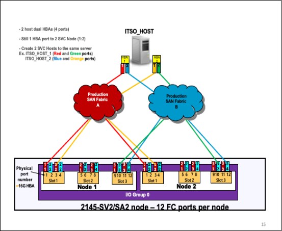
Figure 2-29 4 port host zoning
Because the optimal number of volume paths is four, you must create two or more hosts on the IBM SAN Volume Controller. During volume assignment, alternate which volume is assigned to one of the “pseudo-hosts” in a round-robin fashion.
|
Note: Pseudo-hosts is not a defined function or feature of SAN Volume Controller. To create a pseudo-host, you must add another host ID to the SAN Volume Controller host configuration. Instead of creating one host ID with four WWPNs, you define two hosts with two WWPNs; therefore, you must pay extra attention to the SCSI IDs that are assigned to each of the pseudo-hosts to avoid having two different volumes from the same storage subsystem with the same SCSI ID.
|
ESX cluster zoning
For ESX clusters, you must create separate zones for each host node in the ESX cluster, as shown in Figure 2-30.

Figure 2-30 ESX cluster zoning
Ensure that you apply the following preferred practices to your ESX VMware clustered hosts configuration:
•Zone a single ESX cluster in a manner that avoids ISL I/O traversing.
•Spread multiple host clusters evenly across the IBM SAN Volume Controller node ports and I/O Groups.
•Map LUNs and volume evenly across zoned ports, alternating the preferred node paths evenly for optimal I/O spread and balance.
•Create separate zones for each host node in the IBM SAN Volume Controller and on the ESX cluster.
AIX VIOs: LPM zoning
When zoning IBM AIX® VIOs to IBM Spectrum Virtualize, you must plan carefully. Because of its complexity, it is common to create more than four paths to each volume and MDisk or not provide for proper redundancy. The following preferred practices can help you to have a non-degraded path error on IBM Spectrum Virtualize with four paths per volume:
•Create two separate and isolated zones on each fabric for each LPAR.
•Do not put both the active and inactive LPAR WWPNs in either the same zone or same IBM Spectrum Virtualize host definition.
•Map LUNs to the virtual host FC HBA port WWPNs, not the physical host FCA adapter WWPN.
•When using NPIV, generally make no more than a ratio of one physical adapter to eight Virtual ports. This configuration avoids I/O bandwidth oversubscription to the physical adapters.
•Create a pseudo host in IBM Spectrum Virtualize host definitions that contain only two virtual WWPNs (one from each fabric), as shown in Figure 2-31.
•Map the LUNs/volumes to the pseudo LPARs (active and inactive) in a round-robin fashion.
Figure 2-31 shows a correct SAN connection and zoning for LPARs.

Figure 2-31 LPARs SAN connections
During Live Partition Migration (LPM), both inactive and active ports are active. When LPM is complete, the previously active ports show as inactive and the previously inactive ports show as active.
Figure 2-32 shows a Live partition migration from the hypervisor frame to another frame.

Figure 2-32 Live partition migration
|
Note: During LPM, the number of paths doubles from 4 to 8. Starting with eight paths per LUN or volume results in an unsupported 16 paths during LPM, which can lead to I/O interruption.
|
2.4.6 Hot Spare Node zoning considerations
IBM Spectrum Virtualize V8.1 introduced the Hot Spare Node (HSN) feature that provides a higher availability for SAN Volume Controller clusters by automatically swapping a spare node into the cluster if the cluster detects a failing node. Also the maintenance procedures, like code updates and hardware upgrades, benefit from this feature avoiding prolonged loss of redundancy during the node maintenance.
For more information about hot spare nodes, see IBM Spectrum Virtualize: Hot Spare Node and NPIV Target Ports, REDP-5477.
For the Hot Spare Node feature to be fully effective requires the NPIV feature enabled. In an NPIV enabled cluster, each physical port is associated with two WWPNs. When the port initially logs into the SAN it uses the normal WWPN (primary port), which does not change from previous releases or from NPIV disabled mode. When the node has completed its startup and is ready to begin processing I/O, the NPIV target ports log on to the fabric with the second WWPN.
Special zoning requirements must be considered when implementing the HSN functionality.
Host zoning with HSN
Hosts should be zoned with NPIV target ports only. Spare nodes ports must not be included in the host zoning.
Intercluster and intracluster zoning with HSN
Communications between IBM Spectrum Virtualize nodes, including between different clusters, takes place over primary ports. Spare nodes ports must be included in the intracluster zoning likewise the other nodes.
Similarly, when a spare node comes online, its primary ports are used for Remote Copy relationships and as such must be zoned with the remote cluster.
Back-end controllers zoning with HSN
Back-end controllers must be zoned to the primary ports on lBM Spectrum Virtualize nodes. When a spare node is in use, that nodes ports must be included in the back-end zoning, as with the other nodes.
|
Note: Currently the zoning configuration for spare nodes is not policed while the spare is inactive and no errors will be logged if the zoning or backend configuration is incorrect.
|
Back-end controller configuration with HSN
IBM Spectrum Virtualize uses the primary ports to communicate with the back-end controller, including the spare. Therefore, all MDisks must be mapped to all IBM Spectrum Virtualize nodes, including spares.
For IBM Spectrum Virtualize based back-end controllers, such as IBM Storwize V7000, it is recommended that the host clusters functionality is used, with each node forming one host within this cluster. This configuration ensures that each volume is mapped identically to each IBM Spectrum Virtualize node.
2.4.7 Zoning with multiple IBM SAN Volume Controller clustered systems
Unless two separate IBM SAN Volume Controller systems participate in a mirroring relationship, configure all zoning so that the two systems do not share a zone. If a single host requires access to two different clustered systems, create two zones with each zone to a separate system.
The back-end storage zones must also be separate, even if the two clustered systems share a storage subsystem. You also must zone separate I/O groups if you want to connect them in one clustered system. Up to four I/O groups can be connected to form one clustered system.
2.4.8 Split storage subsystem configurations
In some situations, a storage subsystem might be used for IBM SAN Volume Controller attachment and direct-attach hosts. In this case, pay attention during the LUN masking process on the storage subsystem. Assigning the same storage subsystem LUN to a host and the IBM SAN Volume Controller can result in swift data corruption.
If you perform a migration into or out of the IBM SAN Volume Controller, make sure that the LUN is removed from one place before it is added to another place.
2.5 Distance extension for Remote Copy services
To implement Remote Copy services over distance, the following choices are available:
•Optical multiplexors, such as Dense Wavelength Division Multiplexing (DWDM) or Coarse Wavelength Division Multiplexing (CWDM) devices
•Long-distance SFPs and XFPs
•FC-to-IP conversion boxes
•Native IP-based replication with SAN Volume Controller code
Of these options, the optical varieties of distance extension are preferred. IP distance extension introduces more complexity, is less reliable, and has performance limitations. However, optical distance extension is impractical in many cases because of cost or unavailability.
2.5.1 Optical multiplexors
Optical multiplexors can extend your SAN up to hundreds of kilometers at high speeds. For this reason, they are the preferred method for long-distance expansion. When you are deploying optical multiplexing, make sure that the optical multiplexor is certified to work with your SAN switch model. The IBM SAN Volume Controller has no allegiance to a particular model of optical multiplexor.
If you use multiplexor-based distance extension, closely monitor your physical link error counts in your switches. Optical communication devices are high-precision units. When they shift out of calibration, you start to see errors in your frames.
2.5.2 Long-distance SFPs or XFPs
Long-distance optical transceivers have the advantage of extreme simplicity. Although no expensive equipment is required, a few configuration steps are necessary. Ensure that you use transceivers that are designed for your particular SAN switch only. Because each switch vendor supports only a specific set of SFP or XFP transceivers, it is unlikely that Cisco SFPs work in a Brocade switch.
2.5.3 Fibre Channel over IP
Fibre Channel over IP (FCIP) conversion is by far the most common and least expensive form of distance extension. FCIP is a technology that allows FC routing to be implemented over long distances by using the TCP/IP protocol. In most cases, FCIP is implemented in Disaster Recovery scenarios with some kind of data replication between the primary and secondary site.
FCIP is a tunneling technology, which means FC frames are encapsulated in the TCP/IP packets. As such, it is not apparent to devices that are connected through the FCIP link. To use FCIP, you need some kind of tunneling device on both sides of the TCP/IP link that integrates FC and Ethernet connectivity. Most of the SAN vendors offer FCIP capability through stand-alone devices (multiprotocol routers) or by using blades that are integrated in the director class product. IBM SAN Volume Controller systems support FCIP connection.
An important aspect of the FCIP scenario is the IP link quality. With IP-based distance extension, you must dedicate bandwidth to your FC to IP traffic if the link is shared with other IP traffic. Because the link between two sites is low-traffic or used only for email, do not assume that this type of traffic is always the case. The design of FC is sensitive to congestion and you do not want a spyware problem or a DDOS attack on an IP network to disrupt your IBM SAN Volume Controller.
Also, when you are communicating with your organization’s networking architects, distinguish between megabytes per second (MBps) and megabits per second (Mbps). In the storage world, bandwidth often is specified in MBps, but network engineers specify bandwidth in Mbps. If you fail to specify MB, you can end up with an impressive-sounding 155 Mbps OC-3 link, which supplies only 15 MBps or so to your IBM SAN Volume Controller. If you include the safety margins, this link is not as fast as you might hope, so ensure that the terminology is correct.
Consider the following points when you are planning for your FCIP TCP/IP links:
•For redundancy purposes use as many TCP/IP links between sites as you have fabrics in each site that you want to connect. In most cases, there are two SAN FC fabrics in each site, so you need two TCP/IP connections between sites.
•Try to dedicate TCP/IP links only for storage interconnection. Separate them from other LAN/WAN traffic.
•Make sure that you have a service level agreement (SLA) with your TCP/IP link vendor that meets your needs and expectations.
•If you do not use Global Mirror with Change Volumes (GMCV), make sure that you have sized your TCP/IP link to sustain peak workloads.
•The use of BM SAN Volume Controller internal Global Mirror (GM) simulation options can help you test your applications before production implementation. You can simulate the GM environment within one SAN Volume Controller system without partnership with another. Run the chsystem command with the following parameters to perform GM testing:
– gminterdelaysimulation
– gmintradelaysimulation
For more information about GM planning, see Chapter 6, “Copy services overview” on page 229.
•If you are not sure about your TCP/IP link security, enable Internet Protocol Security (IPSec) on the all FCIP devices. IPSec is enabled on the Fabric OS level, so you do not need any external IPSec appliances.
In addition to planning for your TCP/IP link, consider adhering to the following preferred practices:
•Set the link bandwidth and background copy rate of partnership between your replicating IBM SAN Volume Controller to a value lower than your TCP/IP link capacity. Failing to set this rate can cause an unstable TCP/IP tunnel, which can lead to stopping all your Remote Copy relations that use that tunnel.
•The best case is to use GMCV when replication is done over long distances.
•Use compression on corresponding FCIP devices.
•Use at least two ISLs from your local FC switch to local FCIP router.
•On a Brocade SAN, use the Integrated Routing feature to avoid merging fabrics from both sites.
For more information about FCIP, see the following publications:
•IBM System Storage b-type Multiprotocol Routing: An Introduction and Implementation, SG24-7544
•IBM/Cisco Multiprotocol Routing: An Introduction and Implementation, SG24-7543
2.5.4 SAN extension with Business Continuity configurations
Spectrum Virtualize Enhanced Stretched Cluster and HyperSwap technologies provide Business Continuity solutions over metropolitan areas with distances up to 300 km
(186.4 miles). These Business Continuity solutions over metropolitan areas are achieved by using a SAN extension over WDM technology.
(186.4 miles). These Business Continuity solutions over metropolitan areas are achieved by using a SAN extension over WDM technology.
Furthermore, to avoid single points of failure, multiple WDMs and physical links are implemented. When implementing these solutions, particular attention must be paid in the intercluster connectivity set-up.
|
Important: HyperSwap and Stretched clusters require implementing dedicated private fabrics for the internode communication between the sites. For more information about the requirements, see IBM Spectrum Virtualize HyperSwap SAN Implementation and Design Best Practices, REDP-5597.
|
Consider a typical implementation of an Enhanced Stretched Cluster that uses ISLs, as shown in Figure 2-33.
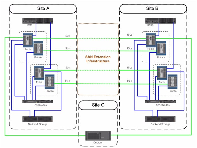
Figure 2-33 Typical Enhanced Stretched Cluster configuration
In this configuration, the intercluster communication is isolated in a Private SAN that interconnects Site A and Site B through a SAN extension infrastructure that consists of two DWDMs. For redundancy reasons, assume that two ISLs are used for each fabric for the Private SAN extension.
Two possible configurations are available to interconnect the Private SANs. In Configuration 1 (see Figure 2-34), one ISL per fabric is attached to each DWDM. In this case, the physical paths Path A and Path B are used to extend both fabrics.

Figure 2-34 Configuration 1: Physical paths shared among the fabrics
In Configuration 2 (see Figure 2-35), ISLs of fabric A are attached only to Path A, while ISLs of fabric B are attached only to Path B. In this case, the physical paths are not shared between the fabrics.

Figure 2-35 Configuration 2: Physical paths not shared among the fabrics
With Configuration 1, in case of failure of one of the physical paths, both fabrics are simultaneously affected and a fabric reconfiguration occurs because of an ISL loss. This situation can lead to a temporary disruption of the intracluster communication and, in the worst case, to a split brain condition. To mitigate this situation, link aggregation features such as Brocade ISL trunking can be implemented.
With Configuration 2, a physical path failure leads to a fabric segmentation of one of the two fabrics, leaving the other fabric unaffected. In this case the intracluster communication would be guaranteed through the unaffected fabric.
Summarizing, the recommendation is to fully understand the implication of a physical path or DWDM loss in the SAN extension infrastructure and implement the suitable architecture to avoid a simultaneous impact.
2.5.5 Native IP replication
It is possible to implement native IP-based replication. Native means that SAN Volume Controller does not need any FCIP routers to create a partnership. This partnership is based on the Internet Protocol network and not on the FC network. For more information about native IP replication, see Chapter 6, “Copy services overview” on page 229.
To enable native IP replication, SAN Volume Controller implements the Bridgeworks SANSlide network optimization technology. For more information about this solution, see IBM SAN Volume Controller and Storwize Family Native IP Replication, REDP-5103.
2.6 Tape and disk traffic that share the SAN
If free ports are available on your core switch, you can place tape devices (and their associated backup servers) on the IBM SAN Volume Controller SAN. However, do not put tape and disk traffic on the same FC HBA.
To avoid any effects on ISL links and congestion on you SAN, do not put tape ports and backup servers on different switches. Modern tape devices have high-bandwidth requirements.
During your backup SAN configuration, use the switch virtualization to separate the traffic type. The backup process has different frames than production and can affect performance.
Backup requests tend to use all network resources that are available to finish writing on its destination target. Until the request is finished, the bandwidth is occupied and does not allow other frames to access the network.
The difference between these two types of frames is shown in Figure 2-36.

Figure 2-36 FC frames access methods
Backup frames uses the sequential method to write data. It releases only the path after it is done writing, while production frames write and read data randomly. Writing and reading is constantly occurring with the same physical path. If backup and production are set up on the same environment, production frames (read and write) can run tasks only when backup frames are complete, which causes latency to your production SAN network.
Figure 2-37 shows one example of a backup and production SAN configuration to avoid congestion because of high bandwidth usage by the backup process.
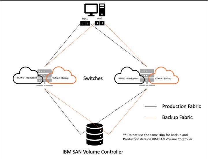
Figure 2-37 Production and backup fabric
2.7 Switch interoperability
SAN Volume Controller is flexible as far as switch vendors are concerned. All of the node connections on a particular SAN Volume Controller clustered system must go to the switches of a single vendor. That is, you must not have several nodes or node ports plugged into vendor A and several nodes or node ports plugged into vendor B.
SAN Volume Controller supports some combinations of SANs that are made up of switches from multiple vendors in the same SAN. However, this approach is not preferred in practice. Despite years of effort, interoperability among switch vendors is less than ideal because FC standards are not rigorously enforced. Interoperability problems between switch vendors are notoriously difficult and disruptive to isolate. Also, it can take a long time to obtain a fix. For these reasons, run only multiple switch vendors in the same SAN long enough to migrate from one vendor to another vendor, if this setup is possible with your hardware.
You can run a mixed-vendor SAN if you have agreement from both switch vendors that they fully support attachment with each other. However, Brocade does not support interoperability with any other vendors.
Interoperability between Cisco switches and Brocade switches is not recommended, except during fabric migrations, and then only if you have a back-out plan in place. Also, when connecting BladeCenter switches to a core switch, consider the use of the N-Port ID Virtualization (NPIV) technology.
When you have SAN fabrics with multiple vendors, pay special attention to any particular requirements. For example, observe from which switch in the fabric the zoning must be performed.
..................Content has been hidden....................
You can't read the all page of ebook, please click here login for view all page.