Dynamics
4.1 Introduction to kinematics
Kinematics is the name given to the study of movement where we do not need to consider the forces that are causing the movement. Usually this is because some aspect of the motion has been specified. A good example of this is the motion of a passenger lift where the maximum acceleration and deceleration that can be applied during the starting and stopping phases are limited by what is safe and comfortable for the passengers. If we know what value this acceleration needs to be set at, then kinematics will allow a design engineer to calculate such things as the time and the distance that it will take the lift to reach its maximum speed.
Before we can get to that stage, however, we need to define some of the quantities that will occur frequently in the study of movement.
Displacement is the distance moved by the object that is being considered. It is usually given the symbol s and is measured in metres (m). It can be the total distance moved from rest or it can be the distance travelled during one stage of the motion, such as the deceleration phase.
Speed is the term used to describe how fast the object is moving and the units used are metres/second (m/s). Speed is very similar to velocity but velocity is defined as a speed in a particular direction. This might seem only a slight difference but it is very important. For example, a car driving along a winding road can maintain a constant speed but its velocity will change continually as the driver steers and changes direction to keep the car on the road. We will see in the next section that this means that the driver will have to exert a force on the steering wheel which could be calculated. Often we take speed and velocity as the same thing and use the symbols v or u for both, but do not forget that there is a distinction. If the object is moving at a constant velocity v and it has travelled a distance of s in time t then the velocity is given by
Alternatively, if we know that the object has been travelling at a constant velocity v for a time of t then we can calculate the distance travelled as
Acceleration is the rate at which the velocity is changing with time and so it is defined as the change in velocity in a short time, divided by the short time itself. Therefore the units are metres per second (the units of velocity) divided by seconds and these are written as metres per second2 (m/s2). Acceleration is generally given the symbol a. Usually the term acceleration is used for the rate at which an object’s speed is increasing, while deceleration is used when the speed is decreasing. Again, do not forget that a change in velocity could also be a directional change at a constant speed.
Having defined some of the common quantities met in the study of kinematics, we can now look at the way that these quantities are linked mathematically.
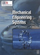
Velocity is the rate at which an object’s displacement is changing with time. Therefore if we were to plot a graph of the object’s displacement s against time t then the value of the slope of the line at any point would be the magnitude of the velocity (i.e. the speed). In Figure 4.1.1, an object is starting from the origin of the graph where its displacement is zero at time zero. The line of the graph is straight here, meaning that the displacement increases at a constant rate. In other words, the speed is constant to begin with and we could measure it by working out the slope of the straight line portion of the graph. The line is straight up to the point where the object has moved by 10 m in 4 s and so the speed for this section is 10 m/4 s = 2.5 m/s. Beyond this section the line starts to become curved as the slope decreases. This shows that the speed is falling even though the displacement is still increasing. We can therefore no longer measure the slope at any point by looking at a whole section of the line as we did for the straight section. We need to work on the instantaneous value of the slope and for this we must adopt the sort of definition of slope that is used in calculus. The instantaneous slope at any point on the curve shown in this graph is ds/dt. This is the rate at which the displacement is changing, which is the velocity and so
In fact the speed goes on decreasing up to the maximum point on the graph where the line is parallel to the time axis. This means that the slope of the line is zero here and so the object’s speed is also zero. The object has come to rest and the displacement no longer changes with time.
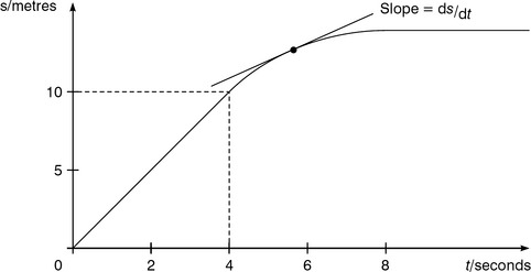
This kind of graph is known as a displacement–time graph and is quite useful for analysing the motion of a moving object. However, an even more useful diagram is something known as a velocity–time graph, such as the example shown in Figure 4.1.2.
Here the velocity magnitude (or speed) is plotted on the vertical axis against time. The same object’s motion is being considered as in Figure 4.1.1 and so the graph starts with the steady velocity of 2.5 m/s calculated above. After a time of 4 s the velocity starts to fall, finally becoming zero as the object comes to rest. The advantage of this type of diagram is that it allows us to study the acceleration of the object, and that is often the quantity that is of most interest to engineers. The acceleration is the rate at which the magnitude of the velocity changes with time and so it is the slope of the line at any point on the velocity–time graph. Over the first portion of the motion, therefore, the acceleration of the object is zero because the line is parallel to the time axis. The acceleration then becomes negative (i.e. it is a deceleration) as the speed starts to fall and the line slopes down.
In general we need to find the slope of this graph using calculus in the way that we did for the displacement–time curve. Therefore
Since v = ds/dt we can also write this as
There is one further important thing that we can get from a velocity–time diagram and that is the distance travelled by the object. To understand how this is done, imagine looking at the object just for a very short time as if you were taking a high-speed photograph of it. The object’s velocity during the photograph would effectively be constant because the exposure is so fast that there is not enough time for any acceleration to have a noticeable effect. Therefore from Equation 4.1.2 the small distance travelled during the photograph would be the velocity at that time multiplied by the small length of time it took to take the photograph. On the velocity–time diagram this small distance travelled is represented by the area of the very narrow rectangle formed by the constant velocity multiplied by the short time, as indicated on the magnified part of the whole velocity–time diagram shown here. If we were prepared to add up all the small areas like this from taking a great many high-speed photographs of all the object’s motion then the sum would be the total distance travelled by the object. In other words the area underneath the line on a velocity–time diagram is equal to the total distance travelled. The process of adding up all the areas from the multitude of very narrow rectangles is known as integration.
Uniform acceleration
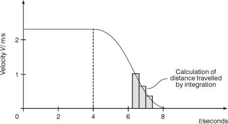
Clearly the analysis of even a simple velocity–time diagram could become quite complicated if the acceleration is continually varying. In this textbook the emphasis is on understanding the basic principles of all the subjects and so from now on we are going to concentrate on the situation where the acceleration is a constant value or at worst a series of constant values. An example of this is shown in Figure 4.1.3.
An object is being observed from time zero, when it has a velocity of u, to time t when it has accelerated to a velocity v. The acceleration a is the slope of the line on the graph and it is clearly constant because the line between the start and the end of the motion is straight. Now the slope of a line, in geometrical terms, is the amount by which it rises between two points, divided by the horizontal distance between the two points. Therefore considering that the line rises by an amount (v − u) on the vertical axis while moving a distance of (t − 0) along the horizontal axis of the graph, the slope a is given by
or
Multiplying through by t gives
and finally
This is the first of four equations which are collectively known as the equations of uniform motion in a straight line. Having found this one it is time to find the other three. As mentioned above, the area under the line on the graph is the distance travelled s and the next stage is to calculate this.
We can think of the area under the line as being made up of two parts, a rectangle representing the distance that the object would have travelled if it had continued at its original velocity of u for all the time, plus the triangle which represents extra distance travelled due to the fact that it was accelerating.
The area of a rectangle is given by height times width and so the distance travelled for constant velocity is ut.
The area of a triangle is equal to half its height times its width. Now the width is the time t, as for the rectangle, and the height is the increase in velocity (v − u). However, it is more useful to note that this velocity increase is also given by at from Equation (4.1.6) as this brings time into the calculation again. The triangle area is then at2/2.
Adding the two areas gives the total distance travelled
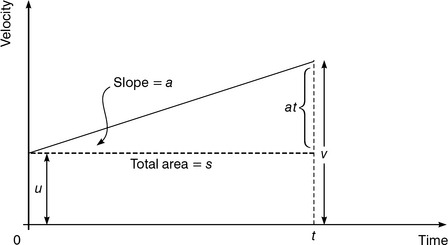
This is the second equation of uniform motion in a straight line. We could have worked out the area under the line on the graph in a different way, however, as shown in Figure 4.1.4.
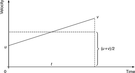
The real area, as calculated above, has now been replaced by a simple rectangle of the same width but with a mean height which is half way between the two extreme velocities, u and v. This is a mean velocity, calculated as (u + v)/2. Therefore the new rectangular area, and hence the distance travelled, is given by
This is the third equation of uniform motion in a straight line and is the last one to involve time t. We need another equation because sometimes it is not necessary to consider time explicitly. We can achieve this by taking two of the other equations and eliminating time from them.
From the first equation we find that
This version of t can now be substituted into the third equation to give
This can be simplified to give finally
This is the fourth and final equation of uniform motion in a straight line. Other substitutions and combinations are possible but these four equations are enough to solve an enormous range of problems involving movement in a line.
Example 4.1.1
An electric cart is to be used to transport disabled passengers between the two terminals at a new airport. The cart is capable of accelerating at a uniform rate of 1.8 m/s2 and tests have shown that a uniform deceleration of 2.4 m/s2 is comfortable for the passengers. Its maximum speed is 4 m/s. Calculate the fastest time in which the cart can travel the distance of 350 m between the terminals.
The first step in solving this problem is to draw a velocity–time diagram, as shown in Figure 4.1.5
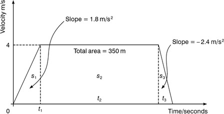
Starting with the origin of the axes, the cart starts from rest with velocity zero at time zero. It accelerates uniformly, which means that the first part of the graph is a straight line which goes up. This acceleration continues until the maximum velocity of 4 m/s is reached. We must assume that there can be a sudden switch from the acceleration phase to the constant velocity phase and so the next part of the graph is a straight line which is parallel to the time axis. This continues until near the end of the journey, when again there is a sudden change to the last phase which is the deceleration back to rest. This is represented by a straight line dropping down to the time axis to show that the cart comes to rest again. We cannot put any definite values on the time axis yet but we can write in that the area under the whole graph line is equal to the distance travelled and therefore has a value of 350 m. Lastly it must be remembered that all the four equations of motion developed above apply to movement with uniform acceleration. The acceleration can have a fixed positive or negative value, or it can be zero, but it must not change. Therefore the last thing to mark on the diagram is that we need to split it up into three portions to show that we must analyse the motion in three sections, one for each value of acceleration.
The overall problem is to calculate the total time so it is best to start by calculating the time for the acceleration and deceleration phases. In both cases we know the initial and final velocities and the acceleration so the equation to use is
We cannot find the time of travel at constant speed in this way and so we must ask ourselves what we have not so far used out of the information given in the question. The answer is that we have not used the total distance yet. Therefore the next step is to look at the three distances involved.
We can find the distance travelled during acceleration using
since we have already calculated the time involved. However, as a point of good practice, it is better to work with the original data where possible and so the first of these two equations will be used.
The distance involved in stopping and starting is
and so
Since this distance relates to constant speed, the time taken for this portion of the motion is simply

Note that, within reason, the route does not have to be a straight line. It must be a fairly smooth route so that the accelerations involved in turning corners are small, but otherwise we can apply the equations of uniform motion in a straight line to some circuitous motion.
Motion under gravity
One of the most important examples of uniform acceleration is the acceleration due to gravity. If an object is allowed to fall in air then it accelerates vertically downwards at a rate of approximately 9.81 m/s2. After falling for quite a time the velocity can build up to such a point that the resistance from the air becomes large and the acceleration decreases. Eventually the object can reach what is called a terminal velocity and there is no further acceleration. An example of this is a free-fall parachutist. For most examples of interest to engineers, however, the acceleration due to gravity can be taken as constant and continuous. They are worthwhile considering, therefore, as a separate case.
The first thing to note is that the acceleration due to gravity is the same for any object, which is why heavy objects only fall at the same rate as light ones. In practice a feather will not fall as fast as a football, but that is simply because of the large air resistance associated with a feather which produces a very low terminal velocity. Therefore we generally do not need to consider the mass of the object. Problems involving falling masses therefore do not involve forces and are examples of kinematics which can be analysed by the equations of uniform motion developed above. This does not necessarily restrict us to straight line movement, as we saw in the worked example, and so we can look briefly at the subject of trajectories.
Example 4.1.2
Suppose a tennis ball is struck so that it leaves the racquet horizontally with a velocity of 25 m/s and at a height above the ground of 1.5 m. How far will the ball travel horizontally before it hits the ground?
Clearly the motion of the ball will be a curve, known as a trajectory, because of the influence of gravity. At first sight this does not seem like the sort of problem that can be analysed by the equations of uniform motion in a straight line. However, the ball’s motion can be resolved into horizontal motion and vertical motion, thus allowing direct application of the four equations that are at our disposal. The horizontal motion is essentially at a constant velocity because the air resistance on a tennis ball is low and so there will be negligible slowing during the time it takes for the ball to reach the ground. The vertical motion is a simple application of falling under gravity with constant acceleration (known as g) since again the resistance will be low and there is no need to consider any terminal velocity. Therefore it is easy to calculate the time taken for the ball to drop by the vertical height of 1.5 m. We know the distance of travel s (1.5 m), the starting velocity u (0 m/s in a vertical sense) and the acceleration a or g (9.81 m/s2) and so the equation to use is
This value can be thought of not just as the time for the ball to drop to the ground but also as the time of flight for the shot. To find the distance travelled along the ground all that needs to be done is to multiply the horizontal velocity by the time of flight.
One of the questions that arises often in the subject of trajectories, particularly in its application to sport, is how to achieve the maximum range for a given starting speed. An example of this would be the Olympic event of putting the shot (Figure 4.1.6), where the athlete might wonder whether it is better to aim high and therefore have a long time of flight or to aim low and concentrate the fixed speed of the shot into the horizontal direction.
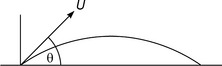
If we suppose the shot starts out with a velocity of u at an angle of θto the ground, then the initial velocity in the vertical direction is u sin θupwards and the constant horizontal velocity is u cosθ. The calculation proceeds like the example above but care has to be taken with the signs because the shot goes upwards in this example before dropping back to the ground. We can take the upwards direction as positive and so the acceleration g will be negative.
By starting with the vertical travel it is possible to work out the time of flight. For simplicity here it is reasonable to neglect the height at which the shot is released and so the shot starts and ends at ground level. In a vertical sense, therefore, the overall distance travelled is zero and the shot arrives back at the ground with the same speed but now in a negative direction. The time of flight tf is therefore twice the time it takes for the shot to reach its highest point and momentarily have a zero vertical velocity.
The horizontal distance travelled is equal to velocity multiplied by time
The actual distance travelled is not of interest, it is simply the angle required to produce a maximum distance that is needed. This depends on finding the maximum value of cos θsin θfor angles between zero (throwing it horizontally) and a right angle (throwing it vertically upwards – very dangerous!). We could do this with calculus but it is just as easy to use common sense which tells us that a sine curve and a cosine curve are identical but displaced by 90° and therefore the product will be a maximum for θ = 45°. In other words, if air resistance can be neglected, it is best to launch an object at 45° to the ground if maximum range is required.
Angular motion
Before leaving the equations of motion and moving on to dynamics, it is necessary to consider angular motion. This includes motion in a circle and rotary motion, both of which are important aspects of the types of movement found in machinery. At first sight it seems that the equations of motion cannot be applied to angular motion: the velocity is continually changing because the direction changes as the object revolves and there is no distance travelled for an object spinning on the spot. However, it turns out that they can be applied directly if a few substitutions are made to find the equivalents of velocity, acceleration and distance.
First the distance travelled needs to be replaced by the angle θ through which the object, such as a motor shaft, has turned. Note that this must be measured in radians, where 1 radian equals 57.3°.
Next the linear velocity needs to be replaced by the angular velocity ω. This is measured in radians per second, abbreviated to rad/s.
Finally the linear acceleration must be replaced by the angular acceleration α which is measured in rad/s2.
The four equations of motion for uniform angular acceleration then become
Example 4.1.3
A motor running at 2600 rev/min is suddenly switched off and decelerates uniformly to rest after 10 s. Find the angular deceleration and the number of rotations to come to rest.
For the first part of this problem, the initial and final angular velocities are known, as is the time taken for the deceleration. The equation to use is therefore:
First it is necessary to put the initial angular velocity into the correct units. One revolution is equal to 2π radians and so 2600 revolutions equals 16337 radians. This takes place in 1 minute, or 60 seconds and so the initial angular velocity of 2600 rev/min becomes 272.3 rad/s.
For the second part the equation to use is
This is not the final answer as it is the number of revolutions that is required. There are 2π radians in one revolution and so this answer needs to be divided by 2 3.141 59, giving a value of 216.7 revolutions.
Motion in a circle
Angular motion can apply not just to objects that are rotating but also to objects that are moving in a circle. An example of this is a train moving on a circular track, as happens in some underground systems around the world. The speed of such a train would normally be expressed in conventional terms as a linear velocity in metres per second (m/s). It could also be expressed as the rate at which an imaginary line from the centre of the track circle to the train is sweeping out an angle like the hands on a clock, i.e. as an angular velocity. The link between the two is
Returning to the original definition of acceleration as either a change in the direction or the magnitude of a velocity, it is apparent that the train’s velocity is constantly changing and so the train is accelerating even though it maintains a constant speed. The train’s track is constantly turning the train towards the centre and so the acceleration is inwards. The technical term for this is centripetal acceleration. It is a linear acceleration (i.e. with units of m/s2) and its value is given by
The full importance of this section will become apparent in the next section, on dynamics, where the question of the forces that produce these accelerations is considered. For the time being just imagine that you are in a car that is going round a long bend. Unless you deliberately push yourself away from the side of the car on the outside of the bend and lean towards the centre, thereby providing the inwards force to accompany the inward acceleration, you will find that you are thrown outwards. Your body is trying to go straight ahead but the car is accelerating towards the geometrical centre of the bend.
Example 4.1.4
A car is to be driven at a steady speed of 80 km/h round a smooth bend which has a radius of 30 m. Calculate the linear acceleration towards the centre of the bend experienced by a passenger in the car.
This is a straightforward application of Equation (4.1.15) but the velocity needs to be converted to the correct units of m/s.
Clearly this is a dramatic speed at which to go round this bend as the passenger experiences an acceleration which is nearly twice that due to gravity. In fact the car would probably skid out of control!
Problems 4.1.1
(1) A car is initially moving at 6 m/s and with a uniform acceleration of 2.4 m/s2. Find its velocity after 6 s and the distance travelled in that time.
(2) A ball is falling under gravity (g = 9.81 m/s2). At time t = 0 its velocity is 8 m/s and at the moment it hits the ground its velocity is 62 m/s. How far above the ground was it at t = 0? At what time did it hit the ground? What was its average velocity?
(3) A train passes station A with velocity 80 km/hour and acceleration 3 m/s2. After 30s it passes a signal which instructs the driver to slow down to a halt. The train then decelerates at 2.4 m/s2 until it stops. Find the total time and total distance from the station A when it comes to rest.
(4) A telecommunications tower, 1000 m high, is to have an observation platform built at the top. This will be connected to the ground by a lift. If it is required that the travel time of the lift should be 1 minute, and its maximum velocity can be 21 m/s, find the uniform acceleration which needs to be applied at the start and end of the journey.
(5) A set of buffers is being designed for a railway station. They must be capable of bringing a train uniformly to rest in a distance of 9 m from a velocity of 12 m/s. Find the uniform deceleration required to achieve this, as a multiple of g, the acceleration due to gravity.
(6) A motor-bike passes point A with a velocity of 8 m/s and accelerates uniformly until it passes point B at a velocity of 20 m/s. If the distance from A to B is 1 km determine:
(7) A light aeroplane starts its take off from rest and accelerates at 1.25 m/s2. It suddenly suffers an engine failure and decelerates back to a halt at 1.875 m/s2, coming to rest after a total distance of 150 m along the runway. Find the maximum velocity reached, and the total time taken.
(8) A car accelerates uniformly from rest at 2 m/s2 to a velocity of V1. It then continues to accelerate up to a velocity of 34 m/s, but at 1.4 m/s2. The total distance travelled is 364 m. Calculate the value of V1, and the times taken for the two stages of the journey.
(9) A large airport is installing a ‘people mover’ which is a sort of conveyor belt for shifting passengers down long corridors. The passengers stand on one end of the belt and a system of sliding sections allows them to accelerate at 2 m/s2 up to a maximum velocity of Vmax. A similar system at the other end brings them back to rest at a deceleration of 3 m/s2. The total distance travelled is 945 m and the total time taken is 60 s. Find Vmax and the times for the three stages of the journey.
(10) A car accelerates uniformly from 14 m/s to 32 m/s in a time of 11.5 s. Calculate:
(11) The same car then decelerates uniformly to come to rest in a distance of 120 m. Calculate:
(12) A train passes a signal at a velocity of 31 m/s and with an acceleration of 2.4 m/s2. Find the distance it travels in the next 10 s.
(13) A piece of masonry is dislodged from the top of a tower. By the time it passes the sixth floor window it is travelling at 10 m/s. Find its velocity 5 s later.
(14) If the total time for the masonry in Problem 13 to reach the ground is 9 s, calculate:
(15) A tram which travels backwards and forwards along Blackpool’s famous Golden Mile can accelerate at 2.5 m/s2 and decelerate at 3.1 m/s2. Its maximum velocity is 35 m/s. Calculate the shortest time to travel from the terminus at the start of the line to the terminus at the other end, a distance of 1580 m, if:
4.2 Dynamics –analysis of motion due to forces
In the chapter on statics we shall consider the situation where all the forces and moments on a body add up to zero. This is given the name of equilibrium and in this situation the body will remain still; it will not move from one place to another and it will not rotate. In the second half of this chapter we shall consider the situation where there is a resultant force or moment on the body and so it starts to move or rotate. This topic is known as dynamics and the situation is described by Newton’s laws of motion which are the subject of most of the first part of this section, where linear motion is introduced.
Most of this section is devoted to the work of Sir Isaac Newton and is therefore known as Newton’s laws of motion. When Newton first published these laws back in the seventeenth century he caused a great deal of controversy. Even the top scientists and mathematicians of the day found difficulty in understanding what he was getting at and hardly anyone could follow his reasoning. Today we have little difficulty with the topic because we are familiar with concepts such as gravity and acceleration from watching astronauts floating around in space or satellites orbiting the earth. We can even experience them for ourselves directly on the roller coaster rides at amusement parks.
Newton lived in the second half of the seventeenth century and was born into a well-to-do family in Lincolnshire. He proved to be a genius at a very early age and was appointed to a Professorship at Cambridge University at the remarkably young age of 21. He spent his time investigating such things as astronomy, optics and heat, but the thing for which he is best remembered is his work on gravity and the laws of motion. For this he not only had to carry out an experimental study of forces but also he had to invent the subject of calculus.
According to legend Newton came up with the concept of gravity by studying a falling apple. The legend goes something like this.
While Newton was working in Cambridge, England became afflicted by the Great Plague, particularly in London. Fearing that this would soon spread to other cities in the hot summer weather, Newton decided to head back to the family’s country estate where he soon found that there was little to do. As a result he spent a great deal of time sitting under a Bramley apple tree in the garden. He started to ponder why the apples were hanging downwards and why they eventually all fell to earth, speeding up as they fell. When one of the apples suddenly fell off and hit him on the head he had a flash of inspiration and realized that it was all to do with forces.
There is some truth in the legend and certainly by the time it was safe for him to return to Cambridge he had formulated the basis of his masterwork. After many years of subsequent work Newton was eventually able to publish his ideas in a finished form. Basically he stated that:
• Bodies will stay at rest or in steady motion unless acted upon by a resultant force.
• A resultant force will make a body accelerate in the direction of the force.
• Every action due to a force produces an equal and opposite reaction.
These are known as Newton’s first, second and third laws of motion respectively.
The first law of motion will be covered fully in Chapter 5 on Statics and so we shall concentrate on the other two. We shall start by looking at the relationship between force, acceleration, mass and gravity. For the time being, however, let us just finish this section by noting that the unit of force, the newton, is just about equal to the weight of one Bramley apple!
Newton’s second law of motion
Let us go back to the legend of Newton and the apple. From the work on statics we will find that the apple stays on the tree as long as the apple stalk is strong enough to support the weight of the apple. As the apple grows there will come a point when the weight is too great and so the stalk will break and the apple falls. The quantity that is being added to the apple as it grows is mass. Sometimes this is confused with weight but there have now been many examples of fruits and seeds being grown inside orbiting spacecraft where every object is weightless and would float if not anchored down.
The reason that the apple hangs downwards on the tree, and eventually falls downwards, is that there is a force of attraction between the earth and any object that is close to it. This is the gravitational force and is directed towards the centre of the earth. We experience this as a vertical, downward force. The apple is therefore pulled downwards by the effect of gravity, commonly known as its weight. Any apple that started to grow upwards on its stalk would quickly bend the stalk over and hang down due to this gravitational effect. As the mass of the apple increases due to growth, so does the weight until the point is reached where the weight is just greater than the largest force that can be tolerated by the stalk. As a result the stalk breaks.
Now let us look at the motion of the apple once it has parted company with the tree. It still has mass, of course, as this is a fundamental property to do with its size and the amount of matter it contains. Therefore it must also have a weight, since this is the force due to gravity acting on the apple’s mass. Hence there is a downwards force on the apple which makes it start to move downwards and get faster and faster. In other words, as we found in the first section of this chapter, it accelerates. What Newton showed was that the force and mass for any body were linked to this acceleration for any kind of motion, not just falling under gravity.
What Newton stated as his Second Law of Motion may be written as follows.
A body’s acceleration a is proportional to the resultant force F on the body and inversely proportional to the mass m of the body.
This seems quite complicated in words but is very simple mathematically in the form that we shall use.
Let us use this first to look at the downward acceleration caused by gravity. The gravitational force between two objects depends on the two masses. For most examples of gravity in engineering one of the objects is the earth and this has a constant mass. Therefore the weight of an object, defined as the force due to the earth’s gravity on the object, is proportional to the object’s mass. We can write this mathematically as
where C is a constant.
Now from Newton’s second law this force W must be equal to the body’s mass m multiplied by the acceleration a with which it is falling.
By comparison between these two equations, it is clear that the acceleration due to gravity is constant, irrespective of the mass of the object. In other words, all objects accelerate under gravity at the same rate no matter whether they are heavy or light. The acceleration due to gravity has been determined experimentally and found to have a value of 9.81 m/s2. It is given a special symbol g to show that it is constant.
The weight of an object is therefore given by
and this is true even if the object is not free to fall and cannot accelerate.
Sometimes this relationship between weight and mass can be confusing. If you were to go into a shop and ask for some particular amount of cheese to be cut for you then you would ask for a specified weight of cheese and it would be measured out in kilograms. As far as scientists and engineers are concerned you are really requesting a mass of cheese; a weight is a force and is measured in newtons.
Before we pursue the way in which this study of dynamics is applied to engineering situations, we must not forget that force is a vector quantity, i.e. it has direction as well as magnitude. Consider the case of two astronauts who are manoeuvring in the cargo bay of a space shuttle with the aid of thruster packs on their backs which release a jet of compressed gas to drive them along (Figure 4.2.1).
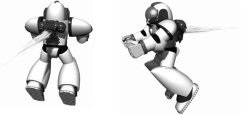
Both packs are the same and deliver a force of 20 N. The first astronaut has a mass of 60 kg and has the jet nozzle turned so it points directly to his left. The second astronaut has a mass of 80 kg and has the nozzle pointing directly backwards. Let us calculate the accelerations produced.
Applying Newton’s second law to the first astronaut
This acceleration will be in the direction of the force, which in turn will be directly opposed to the direction of the nozzle and the gas flow. The astronaut will therefore move to the right.
This acceleration will be away from the jet flow and so it will be directly forward.
This example is very simple because there is no resistance to prevent the acceleration occurring and there are no other forces acting on the astronauts. In general we need to consider friction and we need to calculate the resultant force on a body, as in this next example.
Example 4.2.1
A large mass is being used to raise a smaller mass up a ramp with a cable and pulley system, as shown in Figure 4.2.2. If the coefficient of friction between the small mass and the ramp is 0.3, find the distance travelled by the large mass in the first 25 s after the system is released from rest.
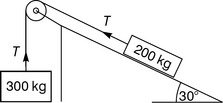
This is an application of Newton’s second law. We need to find the acceleration in order to calculate the distance travelled using the equations of uniform motion that were introduced in the chapter on kinematics. We already know the masses involved and so the remaining step is to calculate the resultant force on the large mass. Clearly the large mass has a weight which will act vertically down and this is given by
This is opposed by the tension force T in the cable which acts upwards and so the resultant downwards force on the large mass is
The acceleration is therefore given by
We can also calculate this acceleration by looking at the other mass, since the two masses are linked and must have the same acceleration. The same tension force will also act equally on the other side of the pulley, which is assumed to be frictionless. There are three forces acting on the smaller mass along the plane of the ramp: the tension force pulling up the slope, the component of the body’s weight acting down the slope and the friction force opposing any motion. The resultant force on the smaller mass is therefore
We therefore have two equations which contain the two unknowns T and a and so we can solve them simultaneously by adding them to eliminate T.
Since we know the acceleration and the time of travel, we can find the distance travelled using the following formula
Rotary motion
In practice most machines involve rotary motion as well as linear motion. This could be such examples as electric motors, gears, pulleys and internal combustion engines. Therefore if we need to calculate how fast a machine will reach full speed (in other words calculate the acceleration of all its components) then we must consider rotary acceleration, and the associated torques, as well as linear acceleration. Fortunately Newton’s second law of motion applies equally well to rotary motion provided we use the correct version of the formula.
Suppose we are looking at the acceleration of a solid disc mounted on a shaft and rotated by a pull cord wrapped around its rim. We cannot use the conventional form of Newton’s second law, F = ma, because although there is a linear force being applied in the form of the tension in the cord, the acceleration is definitely not in a line. We therefore cannot identify an acceleration a in units of m/s2. Furthermore some of the mass of the disc is close to the axle and not moving from one point to another, only turning on the spot, while some of the mass is moving very quickly at the rim. Now in the section on kinematics we saw how the equations of uniform motion could be adapted for rotary motion by substituting the equivalent rotary quantity instead of the linear term. We found that linear distance travelled s could be replaced by angle of rotation θ, while linear acceleration a could be replaced by the angular acceleration α, where α = a/r. It is also quite clear that if we are looking at rotary motion then we should be using the torque τ = Fr instead of force. All that remains is to find the quantity that will be the equivalent of mass in rotary motion.
The mass of an object is really the resistance that the object offers to being moved in a straight line even when there is no friction. It can also be called the inertia of the object; an object with a large mass will accelerate much slower than one with a low mass under the action of an identical force, as we saw in the example of the two astronauts. We are therefore looking for the resistance that an object offers to being rotated in the absence of friction. This must be a combination of mass and shape because a flywheel where most of the mass is concentrated in the rim, supported by slender spokes, will offer much more resistance than a uniform wheel of the same mass. The quantity we are seeking is something known as the mass moment of inertia or simply as the moment of inertia, I, which has units of kilograms times metres squared (kg m2). For a uniform disc, which is the most common shape found in engineering objects such as pulleys, this is given by the formula
We are now in a position to write Newton’s second law in a form suitable for rotary motion
With this equation we can solve problems involving real engineering components that utilize rotary motion and then go on to consider combinations of linear and rotary components.
One of the most common rotary motion devices is the flywheel. This is a massive wheel which is mounted on a shaft to deliberately provide a great deal of resistance to angular acceleration. The purpose of the device is to ensure a smooth running speed, especially for something that is being driven by a series of pulses such as those coming from an internal combustion engine.
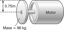
Example 4.2.2
An electric motor is being used to accelerate a flywheel from rest to a speed of 3000 rev/min in 40 s (Figure 4.2.3). The flywheel is a uniform disc of mass 96 kg and radius 0.75 m. Calculate the angular acceleration required and hence find the output torque which must be produced by the motor.
The first part of this problem is an application of kinematics to rotary motion where we know the time, the initial velocity and the final velocity, and we need to find the acceleration. The equation to use is therefore
The start velocity is zero because the flywheel begins from rest. The final angular velocity is
Now that the angular acceleration is known it is possible to calculate the torque or couple which is necessary to produce it, once the moment of inertia is calculated. The flywheel is a uniform disc so the moment of inertia is given by
This general method can be applied to much more complicated shapes such as pulleys which may be regarded as a series of uniform discs on a common axis. Because all the components are all on the same axis, the individual moments of inertia may all be added to give the value for the single shape. Sometimes the moment of inertia of a rotating object is given directly by the manufacturer but there is also another standard way in which they can quote the value for designers. This is in terms of something called the radius of gyration, k. With this the moment of inertia of a body is found by multiplying the mass of the body by the square of the radius of gyration such that
Work, energy and power
So far in this treatment of dynamics we have discussed forces in terms of the accelerations that they can produce but in engineering terms that is only half the story. Forces in engineering dynamics are generally used to move something from one place to another or to alter the speed of a piece of machinery, particularly rotating machinery. Clearly there is some work involved and so we need to be able to calculate the energy that is expended. We start with a definition of work.
To understand this, suppose we have a solid block resting on the floor and a force of F is required to move it slowly against the frictional resistance offered by the floor (Figure 4.2.4).
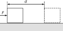
The force is applied for as long as it takes for the mass to be moved by the required distance d. Commonsense tells us that the force must be applied in the direction in which the block needs to move. The work performed is then Fd, which is measured in joules (J). This work is expended as heat which is soon dissipated and is very difficult to recover.
Now suppose we want to lift the same block vertically by a height of h. A force needs to be applied vertically upwards to just overcome the weight mg of the block (remember that weight is a vertical downward force equal to the mass multiplied by the acceleration with which the block would fall down due to gravity if it was unsupported). The mechanical work performed in lifting the block to the required height is therefore
This work is very different from that performed in the first example where it was to overcome friction. Here the work is effectively stored because the block could be released at any time and would fall back to the floor, accelerating as it went. For this reason the block is said to have a potential energy of mgh when it is at a height of h because that amount of work has been carried out at some time in raising it to that level. If the block was now replaced by an item of machinery of the same mass which had been raised piece by piece and then assembled at the top, the potential energy associated with it would still be the same. The object does not have to have been physically raised in one go for the potential energy to be calculated using this equation.
Let us look at another example of potential energy in order to understand better where the name comes from. Suppose you went on a helter-skelter at the fair. You do a great deal of work climbing up the stairs to the top and some of it goes into biological heat. Most of it, however, goes into mechanical work which is stored as potential energy mgh. The reason for the name is that you have the potential to use that energy whenever you are ready to sit on the mat and slide down the chute. Once you are sitting on the mat at the top then you do not need to exert any more force or expend any more energy. You just let yourself go and you accelerate down the chute to the bottom, getting faster all the time. If you had wanted to go that fast on the level then you would have had to use up a great deal of energy in sprinting so clearly there is energy associated with the fact that you are going fast. What has happened is that the potential energy you possessed at the top of the helter-skelter has been converted into kinetic energy. This is the energy associated with movement and is given by the equation
This equation would allow you to calculate your velocity (or strictly your speed) at the bottom of the helter-skelter if there were no friction between the mat on which you have to sit and the chute. In practice there is always some friction and so part of the potential energy is lost in the form of heat. Note that we are not disobeying the conservation of energy law, it is simply that friction converts some of the useful energy into a form that we cannot easily use or recover. This loss of energy in overcoming friction is also a problem in machinery where frictional losses have to be taken into account even though special bearings and other devices may have been used. The way that this loss is included in energy calculations is to introduce the idea of mechanical efficiency to represent how close a piece of mechanical equipment is to being ideal in energy terms.
Machines are always less than 100% efficient and so we never get as much energy out as we put in.
So far we have not included time directly in any of this discussion about work and energy but clearly it is important. Going back to the helter-skelter example, if you were to run up the stairs to the top then you would not be surprised to arrive out of breath. The energy you would have expended would be the same since you end up at rest at the same height, but clearly the fact that you have done it in a much shorter time has put a bigger demand on you. The difference is that in running up the stairs you are performing work faster and therefore operating at a greater power, which is defined as follows
The units of power are joules/second which are also known as watts (W).
This gives us the opportunity to come up with an alternative definition of efficiency. Sometimes it is not possible to measure the total amount of work put into a machine or the total amount of work produced because the machine may be in continuous use. In those circumstances it is possible to think in terms of the rate at which energy is being used and work is being performed. Therefore
This is the definition of mechanical efficiency that is often of most use in the case of rotating machinery so it is appropriate that we should look at how any of these equations could be applied to rotary motion. Using the idea developed in the earlier sections of replacing force F by torque τ, distance moved s by angle of rotationθ, mass m by moment of inertia I and velocity v by angular velocity ω
Example 4.2.3
A farm tractor has an engine with a power output of 90 kW. The tractor travels at a maximum steady speed to the top of a 600 m hill in a time of 4 min 20 s. If the mass of the tractor is 2.4 tonnes, what is the efficiency of the tractor’s drive system?
This is an example of the use of the following equation
The power being put into the drive system of the tractor (i.e. the gearbox, transmission and wheels) is the output power of 90 000 W from the engine. The output power of the drive system can be found from the work involved in raising the tractor up the hill within a given time.
This work is performed in a time of 260 s and so the output power (i.e. the rate of doing work) is

Momentum
When Newton was investigating forces and motion he carried out a series of experiments which involved rolling balls of different masses down inclined planes. This was designed mainly to test his second law of motion concerning forces and accelerations but as part of the experiment he also let the balls collide and measured the result of the collisions. From this he came up with the principle of conservation of momentum. To understand this, let us first look at the concept of momentum.
Suppose you were asked to rate how easy it was to catch the following balls:
You would probably rate the first one the easiest and the last one the most difficult. This is because the tennis ball has small mass and small velocity, whereas the bowling ball in the last case has large mass and large velocity. We found earlier in this chapter that we could think of the mass by itself as inertia, the resistance of an object to being moved, but clearly the mass and the velocity together contribute to the ‘unstopp-ability’ of a moving object. This property of a moving body is known as its momentum, given by
What Newton found in his experiments was that the total momentum of any two balls before a collision was equal to their total momentum after the collision. If we applied this to the third situation described above, but with you standing on a skateboard, then Figure 4.2.5 shows what would happen.
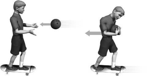
Although you were initially at rest on the skateboard, the act of catching the fast-moving bowling ball would push you backwards slowly. The initial momentum would be mV for the ball but zero for yourself as you are at rest. The final momentum would be equal to the total mass of yourself and the ball (M + m) multiplied by the new, small, common velocity v. The principle of conservation of momentum tells us that
This principle applies to all collisions, however, not just those where the two bodies join together (such as catching the ball). In general the principle of conservation of momentum for two bodies colliding may be stated as
where u refers to velocities before the impact and v refers to velocities after the impact.
This equation is very widely used as it does not only cover the case of two objects colliding, it can handle the situation where two objects are initially united and subsequently separate. Examples of this are shells being fired from guns, stages of a space rocket separating and fuel being ejected from a jet engine. Imagine the special case of two objects that are initially united and are at rest. It could be you on the skateboard again, this time holding the bowling ball. The total momentum would be zero because you are at rest. Now suppose that you throw the ball forward. This would give the ball some forward momentum but, since the total momentum must remain zero, this can only happen if you start to move backwards on the skateboard with equal backwards momentum. What has happened is that you have given the ball an impulse, you have given it forward momentum by pushing it. But at the same time the push has given you an impulse in the opposite direction and it is this that has caused you to move back with equal negative momentum. This is a direct example of Newton’s third law in action. One statement of this law is that
Example 4.2.4
A loaded railway truck of total mass 8600 kg is travelling along a level track at a velocity of 5 m/s and is struck from behind by an empty truck of mass 3500 kg travelling at 8 m/s. The two trucks become coupled together during the collision. Find the velocity of the trucks after the impact.
where V is the common final velocity.
This is quite a simple example in two respects: the trucks join together so there is only a single final velocity and they are both initially moving in the same direction. In general, care has to be taken to make it clear in which direction the objects are moving as it is not always so obvious as in this example. If the two objects were moving towards each other in opposite directions initially then a positive direction would have to be chosen so that one of the objects could be given a positive velocity and the other one a negative velocity. If the two bodies do not start out united or do not join together then there is a major problem in that there are too many unknowns to find from this single equation and another equation is required.
Before we leave this example of the two railway trucks, therefore, it is worthwhile looking at the energy involved. There are only two forms of energy which are of interest in dynamics: kinetic energy and potential energy. For trains on level tracks we can neglect the potential energy as the height of the trucks does not alter. That leaves the kinetic energy to be calculated according to the formula
The initial total kinetic energy is therefore
Clearly some energy was lost in the impact between the two trucks and so the principle of conservation of momentum does not say anythingabout energy being conserved. The question of energy in impacts is left to something called the coefficient of restitution. To understand this, look at the steel ball bouncing on a hard surface in Figure 4.2.6.
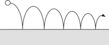
The maximum height of the ball at the top of each bounce gets smaller and smaller as energy is lost in each impact with the hard surface. This shows that the velocity after each impact is less in magnitude than the velocity before the impact. The ratio of the magnitudes of these two velocities is known as the coefficient of restitution e which clearly always has a value of less than one. For simplicity it is best to define e in terms of speed since then we do not have to take into account the fact that the ball changes direction at each bounce.
The idea of using relative speeds is to make it applicable to cases where both bodies are moving before and after the impact, unlike the simple case above where the hard surface is fixed.
Example 4.2.5
A ball of mass 12 kg is moving at a speed of 2 m/s along a smooth surface. It is hit from behind by a ball of the same diameter but a mass of only 4 kg travelling in the same direction with a speed of 8 m/s. The coefficient of restitution between the two balls is 0.75. Calculate the final velocities of the two balls.
First we apply the principle of conservation of momentum
Next we apply the coefficient of restitution
We now have two equations relating the two final velocities and so we can solve them simultaneously or simply make a substitution. Finally this gives us
Angular momentum
Before we leave the topic of momentum, we should again consider how the equations that we have learned for linear motion apply to rotary motion. We have already seen that the linear velocity v in m/s can be replaced by the angular velocity ω in rad/s, such that v = rω. We have also seen that the equivalent of mass m in kg in rotational terms is the moment of inertia I in kgm2. It follows from this that the rotational equivalent of momentum mv is the angular momentum Iω.
The principle of conservation of angular momentum then becomes
where the symbol Ω is used for the final angular velocities.
Problems with angular momentum are solved in exactly the same way as those for linear momentum except that there is rarely any need to use a coefficient of restitution. This is because problems generally involve a single object which changes its shape and therefore its moment of inertia. An example would be a telecommunications satellite which is needed to spin in its final position in space. Usually this is achieved by spinning the satellite while it is still attached to its anchor points in the cargo bay of a space shuttle. The difficulty is that the satellite will unfold very long solar panels once it is released and this will increase its moment of inertia. The engineers in charge of the project will solve the problem by calculating the final momentum with the panels unfolded as well as the initial moment of inertia with the panels folded away. Using the principle of conservation of angular momentum and knowing the final angular velocity required, it is straightforward to calculate the initial angular velocity that must be reached before the satellite can be released.
Example 4.2.6
A telecommunications satellite has a moment of inertia of 82 kg m2 when it is in its final configuration with its solar panels extended. It is required to rotate at a rate of 0.5 rev/s in this configuration. When the satellite is still in the cargo bay of a shuttle vehicle and the panels are still folded away, it has a moment of inertia of 6.8 kg m2. To what rotational speed should it be accelerated before being released and unfolded.
d’Alembert’s principle
The final section in this chapter is really more to do with statics, surprisingly, and concerns a way of tackling dynamics problems that was devised by a French scientist called d’Alembert. At the time of its introduction it was very difficult to understand but nowadays we are all familiar with some of its applications in space travel. Suppose we consider the case of astronauts being launched into space on a space shuttle. During the launch when the shuttle is vertical and accelerating rapidly up through the atmosphere with the rockets at full blast, the astronauts feel as though they have suddenly become extremely heavy; they cannot raise their arms from the arms of the seat, they cannot raise their heads from the headrests and the skin on their faces is pulled back tight because it is apparently so heavy. We know that all this is because the shuttle is accelerating so fast that the astronauts are subjected to what are known as ‘g-forces’, the sort of forces you feel on a roller coaster as it goes through the bottom of a tight curve. However, if you were in the space shuttle and the windows were blacked out so that you could not see any movement, you could be excused for thinking that the astronauts really were being subjected to some large extra force acting in the opposite direction to the acceleration. For an astronaut of mass m experiencing an acceleration of a directly upwards, the extra imaginary force would be F = ma directly down, according to Newton’s second law. From that point on, any engineering dynamics problem concerning the astronaut, such as working out the reaction loads on the seat anchor points, could be carried out as a statics calculation with this imaginary force included. This is d’Alembert’s principle.
Problems 4.2.1
(1) A car of mass 1200 kg accelerates at a rate of 2.8 m/s2. Calculate the resultant driving force which must be acting on it.
(2) A force of 5.4 kN is used to accelerate a fork-lift truck of mass 1845 kg. Calculate the acceleration produced.
(3) A man exerts a horizontal force of 300 N to push a trolley. If the trolley accelerates at 0.87 m/s2, calculate its mass.
(4) A car of mass 1.4 tonnes rests on a 30° slope. If it were allowed to roll down the hill, what would be its acceleration? Assume that the resistance to motion is equivalent to a force of 1000 N acting up the hill.
(5) Two masses are connected by a light cable passing over a frictionless pulley (Figure 4.2.7). If they are released from rest calculate their initial acceleration:
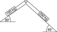
Figure 4.2.7
(6) Two masses are connected as shown in Figure 4.2.8 by a light cable passing over a frictionless pulley. If the coefficient of friction between the mass and the incline is 0.28 find the distance that the large mass falls in the first 30 s after the system is released from rest.
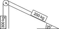
Figure 4.2.8
(7) Calculate the acceleration of the two bodies shown in Figure 4.2.9 if the coefficient of friction on the slope is 0.24.
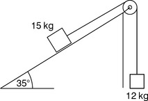
Figure 4.2.9
(8) Calculate the acceleration if the coefficient of friction on the slope shown in Figure 4.2.10 is 0.32:
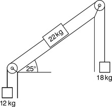
Figure 4.2.10
(9) Calculate the acceleration of the two bodies shown in Figure 4.2.11:
Figure 4.2.11
(10) A harrier jump-jet has a mass of 12 500 kg when fully laden and can take off vertically with an acceleration of 4 m/s2. It then switches to forward flight, while maintaining constant thrust, and initially experiences an air resistance force of 20 kN. Calculate the horizontal acceleration and hence find the distance travelled in the first 15 s of horizontal flight.
(11) A helicopter can accelerate vertically upwards at a rate of 3.5 m/s2 when it is unloaded and has a mass of 2250 kg. Calculate the maximum extra load it could support.
(12) A lunar landing module of mass 5425 kg, including crew and fuel, etc., is designed for a maximum deceleration of 5.6 m/s2 when using half thrust on its rocket motors during a landing on the moon. While on the moon 100 kg of fuel is used, 200 kg of rubbish are jettisoned and 450 kg of equipment are left behind. Calculate the acceleration on take-off at full power.
(13) By the time the module in Problem 12 has reached orbit around the moon, it has used another 675 kg of fuel. Calculate the acceleration it could then achieve at three-quarters thrust.
(14) A lift cage has a mass of 850 kg and the tension in the cable when the lift is moving upwards at a steady velocity with six people inside it, each of mass 150 kg, is 20 kN. Assuming that friction is constant, calculate the tension in the cable when the same lift containing only four of the people accelerates upwards from rest at a rate of 2 m/s2.
(15) An electric motor with a moment of inertia 118.3 kg m2 experiences a torque of 249 Nm. Calculate the angular acceleration of the motor under no-load conditions, and hence find the time to reach a speed of 3600 rpm from rest, assuming the acceleration remains uniform.
(16) A motor is used to accelerate a flywheel from rest to a speed of 2400 rpm in 32 s. The flywheel is a disc of mass 105 kg and radius 0.85 m. Calculate the angular acceleration required and hence find the output torque which must be produced by the motor.
(17) A locomotive turntable is a horizontal disc of diameter 20 m and mass 105 tonnes, which is evenly distributed. It needs to reach its maximum speed of 1 rpm within 20 s when it is unloaded and the resistance due to friction is equivalent to a force of 102 N acting tangentially at the edge of the turntable. Calculate the driving torque required.
(18) A pulley on a shaft (Figure 4.2.12) can be considered as a number of discs mounted on the same axis. If the density of the material is 7800 kg/m3, calculate the moment of inertia of the pulley and shaft, and hence find the torque required to accelerate it from rest to a speed of 5400 rpm in 12 s.
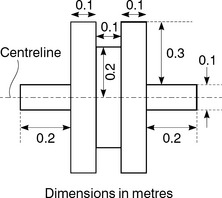
Figure 4.2.12
(19) A flywheel is constructed as shown in Figure 4.2.13. By considering it as a number of discs, both real and imaginary, calculate its moment of inertia. Hence calculate the time it will take to reach a speed of 4800 rpm if the torque which can be applied to give a uniform acceleration is 206 Nm. Density of the material is 8200 kg/m3.
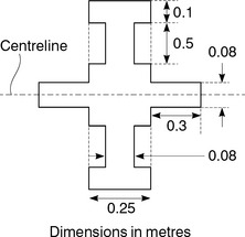
Figure 4.2.13
(20) A winding drum with a built-in flywheel is attached to a suspended mass of 110 kg by a light cord. The drum diameter is 0.2 m and the moment of inertia of the assembly is 59 kg m2. Calculate the distance that the mass will fall in 9 s if it is released from rest.
(21) For the same arrangement, what torque must be applied to the drum to accelerate the mass upwards from rest at a rate of 2 m/s2.
(22) A truck is hauled up a slope by a cable system which is driven by an electric motor (Figure 4.2.14); but also has a counterweight as shown. If the resistance to motion of the truck is 800 N, calculate the torque that the motor must apply at the winding drum in order to pull the truck up the slope a distance of 10 m from rest in 8 s.
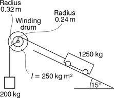
Figure 4.2.14
(23) The waterside at Niagara Falls can be reached by a cable car which moves up and down the side of the gorge (Figure 4.2.15). If the motor which drives it were to fail, calculate the time it would take to move 50 m up the slope, and find the braking force which would need to be applied to the car subsequently to bring it back to rest at the top of the slope.
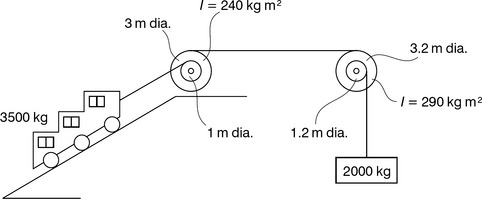
Figure 4.2.15
(24) Calculate the work required to move a packing case along the floor by 18.5 m if the force required to overcome friction is 150 N.
(25) How much work is required to raise a 26 kg box by 16 m?
(26) How much kinetic energy does a car of mass 1.05 tonnes have at a speed of 80 km/hour?
(27) A lump of lead, of mass unknown, is dropped from a tower. Because of air resistance the conversion of its potential energy to kinetic energy is only 86% efficient. Calculate its velocity after it has fallen by 9 m.
(28) A crossbow exerts a steady force of 400 N over a distance of 0.15 m when firing a bolt, of mass 0.035 kg. If the crossbow is 76% efficient, calculate the velocity of the bolt as it leaves the bow.
(29) An electric motor of 60 W power drives a winch which can raise a 10 kg mass by 15 m in 29.9 s. Calculate the efficiency of the winch.
(30) A railway wagon has a velocity of 20 m/s as it reaches the start of an inclined track (angle of elevation 1.2°). How far will it travel up the inclined track, if all resistance can be neglected and it is allowed to freewheel until it comes to rest?
(31) For the same situation as Problem 30, what will be the velocity of the wagon after it has travelled 200 m up the slope?
(32) If the wagon is only 75% efficient at converting kinetic energy to potential energy when freewheeling, calculate its velocity after it has travelled 300 m up the incline.
(33) A car has an engine with a power output of 46 kW. It can travel at a steady speed to the top of a 500 m high hill in 3 min 42 s. How efficient is the car if its mass is 1.45 tonnes?
(34) A 24 kg shell is fired from a 4 m long vertical gun barrel, and reaches a velocity of 450 m/s as it leaves the gun. Calculate:
(a) the constant force propelling it along the barrel;
(b) the maximum height above ground level reached by the shell;
(c) the speed at which it strikes the ground on return.
Assume an average constant resistance due to the air of 45 N once the shell is out of the gun.
(35) The resistance to motion of a car of mass 850 kg can be found using the formula Resistance = 1.2 V2 newtons, where V is the car’s velocity in m/s. Calculate the power required from the car’s engine to produce speeds of 5, 15 and 30 m/s:
(a) along the straight horizontal track;
(b) ascending a slope of sin−1 0.1.
In all cases also calculate the total work done by the tractive force over a distance of 1 km.
(36) A bullet is fired into a sand box suspended on four wires as shown in Figure 4.2.16, and becomes embedded in the sand. The sand box has a mass of 10 kg; the bullet has a mass of 0.01 kg. Only 1% of the bullet’s energy goes towards moving the box; the rest is dissipated in the sand. If θ= 18° for the furthest point of the swing, estimate the velocity of the bullet just before it strikes the box.
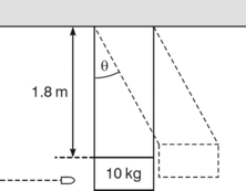
Figure 4.2.16
(37) Water of density 1000 kg/m3 is to be raised by a pump from a reservoir through a vertical height of 12 m at a rate of 5 m3/s. Calculate the required power of the pump, neglecting any energy loss due to friction.
(38) Water emerges from a fire hose in a 50 mm diameter jet at a speed of 20 m/s. Calculate the power of the pump required to produce this jet and estimate the vertical height the jet would reach.density of water = 1000 kg/m3;flow rate in kg/s = jet area velocity density
(39) A body of mass m is at rest at the top of an inclined track of slope 30°. It is released from rest and moves down the slope without friction. Calculate its speed after it has moved 20 m by using the energy method and by using the equation for motion in a straight line.
(40) The body from Problem 39 now starts from rest and moves down another 30° slope, but this time against a friction force of 20 N. Calculate its speed after it has moved 20 m down this slope, again using both methods.
(41) A body of mass 30 kg is projected up an inclined plane of slope 35° with an initial speed of 12 m/s. The coefficient of friction between body and plane is 0.15. Calculate using the energy method:
(a) how far up the slope it travels before coming to rest;
(b) how fast it is travelling when it returns to its initial position.
(42) Two railway trucks, as shown in Figure 4.2.17, collide and become coupled together. Find the velocity of the two trucks after the collision.
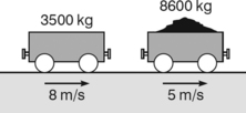
Figure 4.2.17
(43) Two spacecraft, moving in the same direction, are about to undertake a docking manoeuvre (Figure 4.2.18). Find the final velocity of the two craft if the manoeuvring rockets fail and the docking becomes more like a collision.
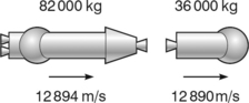
Figure 4.2.18
(44) A large gun is mounted on a railway wagon which is travelling at 5 m/s. The total mass is 3850 kg. The gun fires a 5 kg shell horizontally at a velocity of 1050 m/s back along the track. Find the new velocity of the wagon, which you may assume to be freewheeling.
(45) Two railway wagons are approaching each other from opposite directions, one with mass 1200 kg moving at a velocity of 2 m/s and the other with mass 1400 kg and velocity 3 m/s. If the wagons lock together at collision, find their common velocity finally.
(46) A man of mass 82 kg is skating at 5 m/s carrying his partner, a woman of mass 53 kg, as part of an ice dancing movement. He then throws her forward so that she moves off at 5.9 m/s. Find the man’s velocity just after the throw.
(47) A ball of mass 4 kg and moving at 8 m/s collides with a ball of mass 12 kg moving in the opposite direction at 2 m/s. If the coefficient of restitution between them is 0.75, find the final velocities.
(48) A railway wagon of mass 120 kg and moving at a velocity of 8 m/s runs into the back of a second wagon of mass 180 kg moving in the same direction at 6 m/s. If the coefficient of restitution is 0.8, find the final velocities.
(49) A satellite of mass 40 kg and travelling at a speed of 5 m/s accidentally collides with a larger satellite of mass 80 kg. It rebounds and moves in the opposite direction at a speed of 5 m/s. If the coefficient of restitution between the two satellites is 0.8, find the initial velocity of the larger satellite.