
Fluid mechanics
3.1 Hydrostatics – fluids at rest
The first half of this chapter is devoted to hydrostatics, the study of fluids at rest. It is a subject that is most commonly associated with civil engineers because of their interest in dams and reservoirs, but it is necessary for mechanical engineers too as it leads on to the subject of hydrodynamics, fluids in motion.
What are fluids?
Fluids are any substances which can flow. We normally think of fluids as either liquids or gases, but there are also cases where solids such as fine powders can behave as fluids. For example, much of the ground in Japan is made up of fine ash produced by the many volcanoes which were active on the islands until quite recently. Earthquakes are still common there and the buildings run the risk of not only collapsing during the tremors but also sinking into the ground as the powdery ash deposits turn into a sort of fluid due to the vibration. Nevertheless we shall only consider liquids and gases for simplicity, and most of the time we shall narrow the study down even further to liquids because we can look at the basic principles without the complications that apply to gases because of their compressibility. There are only a few major differences between liquids and gases, so let us have a look at them first.
Liquids and gases
It is easiest if we arrange the differences between liquids and gases as a double list (see Figures 3.1.1–3.1.6).


From this list of differences it is plain to see that it is much easier to study liquids, and so that is what we shall do most of the time since the basic principles of fluid mechanics apply equally well to liquids and gases. There is only one instance where liquids are more complicated to study than gases and that is to do with the fact that liquids are much more dense.
Pressure in liquids
The drawback to this approach of concentrating on liquids is that liquids are very dense compared with gases and so we do not have to go very far down into a liquid before the pressure builds up enormously due to the weight of all the mass of liquid above us. This variation of pressure with depth is almost insignificant in gases. If you were to climb to the top of any mountain in the UK then you would not notice any difference in air pressure even though your altitude may have increased by about 1000 metres. In a liquid, however, the difference in pressure is very noticeable in just a few metres of height (or depth) difference. Anyone who has ever tried to swim down to the bottom of a swimming pool will have noticed the pressure building up on the ears after just a couple of metres. This phenomenon is, of course, caused by gravity which makes the water at the top of the swimming pool press down on the water below, which in turn presses down even harder on the ears. In order to quantify this increase of pressure with depth we need to look at the force balance on a submerged surface, so let us make that surface an ear drum, as shown in Figure 3.1.7
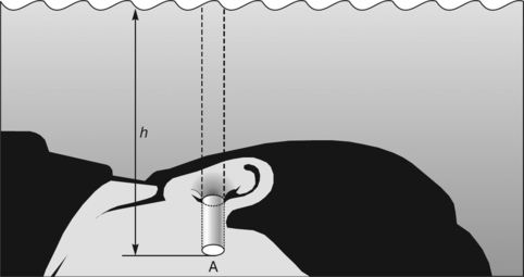
We are dealing with gravitational forces, which always act vertically, and so we only need to consider the effect of any liquid, in this case water, which is vertically above the ear drum. Water which is to either side of the vertical column drawn in the diagram will not have any effect on the pressure on the ear drum, it will only pressurize the cheek or the neck, etc.
The volume of water which is pressing down on the ear drum is the volume of a cylinder of height h, equal to the depth of the ear, and end area A, equal to the area of the ear drum,
Therefore the mass of water involved is
Volume × density = ρhA where ρis the density in kg/m3
We are interested in the pressure p rather than this force, so that we can apply the result to any shaped surface. This pressure will be uniform across the whole of the area of the ear drum and we can therefore rewrite the force due to the water as pressure × area. Hence:
Cancelling the areas we end up with:
Since the area of the eardrum cancelled out, this result is not specific to the situation we looked at; this equation applies to any point in any liquid. We can therefore apply this formula to calculate the pressure at a given depth in any liquid in an engineering situation. There are two further important features that need to be stressed:
• Two points at the same depth in the same liquid must be at the same pressure even if one of them is not directly underneath the full depth (Figure 3.1.8).

• The same pressure due to depth can be achieved with a variety of different shaped columns of a liquid since only the vertical depth matters (Figure 3.1.9).

Pressure head
We can relate a liquid’s pressure to the height of a column of that liquid whether there really is a column there or not. We could be producing the pressure with a pump, for example, but it can still be useful to talk in terms of a height of liquid since this is a simple measurement which is easier to understand and visualize than the correct units of pressure (pascals or N/m2). This height can be calculated by rearranging Equation (3.1.1) to give
and it is known as the pressure head or the static head (since it refers to liquids at rest). The idea of ‘head’ comes from the early British engineers who built canals and reservoirs, and realized that the amount of pressure or even power they could get from the water depended on the vertical height difference between the reservoir surface and the place where they were working. The idea was taken up by the steam engineers of the Victorian era who talked about the ‘head of steam’ they could produce in a boiler, and it is such a useful concept that it is still used today even though it sounds old fashioned.
In order to get a better understanding of the meaning of a head, and to gain practice in converting from head to pressure, we shall now look at ways of using the height of a column of liquid to measure pressure.
Manometry
Manometry is the measurement of pressure using columns of liquid, although more modern electronic pressure measurement devices often also get called manometers. Liquid manometers are still widely used for pressure measurement and so this study is far from being of just historical interest. They are used in a great many configurations, so the four examples we shall look at here are just illustrations of how to go about calculating the conversions from a height of liquid in metres to a pressure in pascals.
Piezometer tube (or simple manometer tube) (Figure 3.1.10)
The pressurized liquid in the horizontal pipe rises up the vertical glass tube until the pressure from the pipe is balanced by the pressure due to the column of liquid, and the liquid comes to rest. At that point the pressure head is simply the height of the liquid in the tube, measured from the centreline of the pipe. The pressure in the pipe can be found from the formula
where ρis the density of the liquid filling the pipe and the manometer tube. This is a beautifully simple device that is inherently accurate; as mentioned earlier it is only the vertical height that matters so any inclination of the tube or any variation in diameter does not affect the reading so long as the measuring scale itself is vertical. In practice the piezometer tube is limited to measuring heads of about 1 metre because otherwise the glass tube would be too long and fragile.

U-tube manometer (Figure 3.1.11)
For higher pressures we can use a higher density liquid in the tube. Clearly the choice of liquids must be such that the liquid in the tube does not mix with the liquid in the pipe. Mercury is the most commonly used liquid for the manometer tube because it has a high density (relative density of 13.6, i.e. mercury is 13.6 times denser than water) and it does not mix with common liquids since it is a metal. To prevent it escaping from the manometer tube a U-bend is used.
Note that in the diagram the height of the mercury column is labelled as x and not as h. This is because the head is always quoted as the height of a column of the working liquid (the one in the pipe), rather than the measuring liquid (the one in the manometer tube). We therefore need to convert from x to obtain the head of working liquid that would be obtained if we could build a simple manometer tube tall enough. To solve any conversion problem with manometers it is usually best to work from the lowest level where the two liquids meet, in this case along the level AA’.
Pressure at A is due to the left-hand column so
Pressure at A’ is partly due to the right-hand column and partly due to the pressure in the pipe, so
We can interpret the pressure in the pipe as a pressure head using pwl = ρwlghwl
Now we know that the pressure in a liquid is constant at a constant depth, so the pressure at A must equal the pressure at A’ just inside the mercury. Therefore
To simplify this and find the pressure head:
Example 3.1.1
A U-tube manometer containing mercury of density 13600 kg/m3 is used to measure the pressure head in a pipe containing a liquid of density 850 kg/m3. Calculate the head in the pipe if the reading on the manometer is 245 mm and the lower meniscus is 150 mm vertically below the centreline of the pipe.
The set-up is identical to the manometer shown in Figure 3.1.11 and so we can use Equation (3.1.2) directly. Remember to convert any measurements in millimetres to metres.

Differential inverted U-tube manometer
In many cases it is not just the pressure that needs to be measured, it is the pressure difference between two points that is required. This can often be measured directly by connecting a single manometer to the two points and recording the differential head, as shown in Figure 3.1.12.
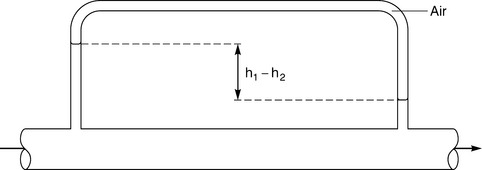
Since it is the working liquid itself that fills the manometer tubes and there is no separate measuring liquid, the head difference is given directly by the difference in the heights in the tubes (h1 − h2). In this case the difference is limited again to about 1 metre because of the need for a glass tube in order to see the liquid levels.
Differential mercury U-tube manometer (Figure 3.1.13)
To make it possible to record higher differential pressures, again we can use mercury for the measuring liquid, giving a device which is by far the most common form of manometer because of its ability to be used on various flow measuring devices.
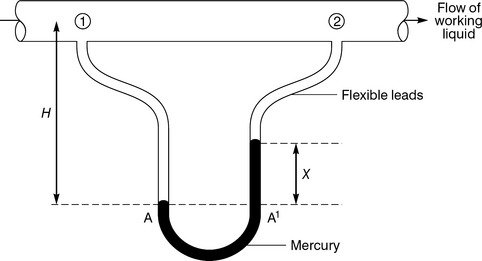
Again we tackle the problem of converting from the reading x into the head difference of the working liquid (h1 − h2) by working from the lowest level where the two liquids meet. So we start by equating the pressures at A and A’ (i.e. at the same depth in the same liquid).
Pressure at A is equal to the pressure at point 1 in the pipe plus the pressure due to the vertical height of the column of working liquid in the left-hand tube: p1 + ρwlgH.
Pressure at A’ is equal to the pressure at point 2 in the pipe plus the pressure due to the vertical height of the short column of working liquid sitting on the column of mercury in the right-hand tube:
Rewriting the pressure terms to get heads h1 and h2, and equating the pressures at A and A’ we get:
Cancel g because it appears in all terms and cancel the term pwlgH because it appears on both sides.
Finally we have
This equation is well worth learning because it is such a common type of manometer, but remember that it only applies to this one type.
Example 3.1.2
A mercury U-tube manometer is to be used to measure the difference in pressure between two points on a horizontal pipe containing liquid with a relative density of 0.79. If the reading on the manometer scale for the difference in height of the two levels is 238 mm, calculate the head difference and the pressure difference between the two points.
We can use Equation (3.1.3) directly to solve this problem and give the head difference, but remember to convert millimetres to metres (divide by 1000) and convert relative density to real density (multiply by 1000 kg/m3).

The pressure difference is found by using p = ρgh and remembering that the density to use is the density of the liquid in the pipeline; once we have converted from x to h in the first part of the calculation then the mercury plays no further part.
Hydrostatic force on plane surfaces
In the previous section we looked at the subject of hydrostatic pressure variation with depth in a liquid, and used the findings to explore the possibilities for measuring pressure with columns of liquids (manometry). In this section we are going to extend this study of hydrostatic pressure to the point where we can calculate the total force due to liquid pressure acting over a specified area. One of the main reasons that we study fluid mechanics in mechanical engineering is so that we can calculate the size of forces acting in a situation where liquids are employed. Knowledge of these forces is essential so that we can safely design a range of devices such as valves, pumps, fuel tanks and submersible housings. Although we shall not look at all the many different situations that can arise, it is vital that you understand the principles involved by studying a few of the most common applications.
Hydraulics
The first thing to understand is the way that pressure is transmitted in fluids. Most of this is common sense but it is worthwhile spelling it out so that the most important features are made clear.
Look at Figures 3.1.14 and 3.1.15. In Figure 3.1.14 a short solid rod is being pushed down onto a solid block with a force F. The cross-sectional area of the rod is A and so a localized pressure of
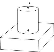
is felt underneath the base of the rod. This pressure will be experienced in the block mainly directly under the rod, but also to a much lesser extent in the small surrounding region. It will not be experienced in the rest of the solid block towards the sides.
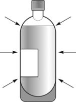
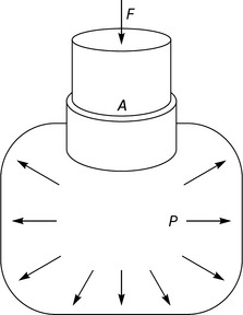
Now look at Figure 3.1.15 where the same rod is used as a piston to push down with the same force on a sealed container of liquid. The result is very different because the pressure of
will now be experienced by all the liquid equally. If the container were to spring a leak we know that the liquid would spurt out normal to the surface that had the hole in it. If the leak were in the top surface of the container then the liquid would spurt upwards, in completely the opposite direction to the force that is being applied to the piston. This means that the liquid was being pushed in that upwards direction and that can only happen if the pressure acts normally to the inside surface.
This simple imaginary experiment therefore has two very important conclusions:
• Pressure is transmitted uniformly in all directions in a fluid.
• Fluid pressure acts normal (i.e. at right angles) to any surface that it touches.
These two properties of fluid pressure are the basis of all hydraulic systems and are the reason why car brakes work so successfully. The force applied by the driver’s foot to the small cross-section piston and cylinder produces a large pressure in the hydraulic fluid that completely fills the system. This large pressure is transmitted along the hydraulic pipes under the car to the larger area pistons and cylinders at the wheels where it produces a large force that operates the brakes themselves. The force on the piston faces is at right angles to the face and therefore exactly in the direction where it can have most effect.
The underlying principle behind hydraulics is that by applying a small force to a small area piston we can generate a large pressure in the hydraulic fluid that can then be fed to a large area piston to produce an enormous force. The reason that this principle works is that the hydraulic fluid transmits the applied pressure uniformly in all directions, as we saw above.
It sometimes seems as though we are getting something for nothing in examples of hydraulics because small, applied forces can be used to produce very large output forces and shift massive objects such as cars on jacks. Of course we cannot really get something for nothing and the penalty that we have to pay is that the small piston has to be replaced by a pump which is pushed backwards and forwards many times in order to displace the large volume of fluid required to make the large piston move any appreciable distance. This means that the small force on the driving piston is applied over a very large distance (i.e. many times the stroke length of the pump) in order to make the large force on the big piston move through one stroke length, as illustrated in Figure 3.1.16.
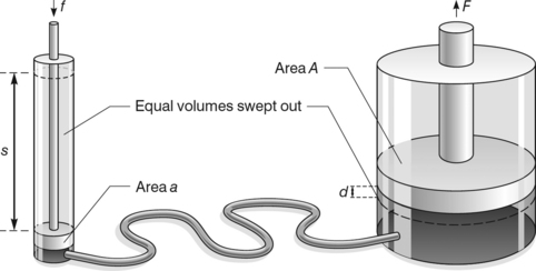
The volume of hydraulic fluid expelled by the small piston in one stroke is given by:
where s and a are the stroke length and area of the small piston respectively.
The work done by the piston during this stroke is given by:
This volume of fluid expelled travels to the large cylinder, which moves up by some distance d such that the extra volume in the cylinder is given by:
The work done on the load on the large piston is given by: Work
Now the volume expelled from the small cylinder is the same as the volume received by the large cylinder, because liquids are incompressible for all practical purposes, therefore:
So Workout = Fsa/A = Psa = fs = Workin. (Note: pressure is uniform so P = f/a = F/A.)
In practice there would be a slight loss of energy due to friction and so it is clear that hydraulic systems actually increase the amount of work to be done rather than give us something for nothing, but their big advantage is that they allow us to carry out the work in a manner which is more convenient to us.
Example 3.1.3
A small hydraulic cylinder and piston, of diameter 50 mm, is used to pump oil into a large vertical cylinder and piston, of diameter 250 mm, on which sits a lathe of mass 350 kg. Calculate the force which must be applied to the small piston in order to raise the lathe.
The pressures in the two cylinders must be equal and so
Where the lower case refers to the small components and the upper case refers to the large components. We are trying to find the small force f and we do not need to calculate P, so this equation can be rearranged:
The large force F is equal to the mass of the lathe multiplied by the acceleration due to gravity, i.e. it is the lathe’s weight. The two areas do not need to be calculated because the ratio of areas is equal to the square of the ratio of the diameters. Note that we do not need to convert the millimetres to metres in the case of a ratio. Therefore

Pressure on an immersed surface
We now need to look at fluid forces in a more general way. Suppose that you were required to design a watertight housing for an underwater video camera that is used to traverse up and down the legs of a giant oil rig looking for structural damage, as shown in Figure 3.1.17.

In order to specify the thickness, and hence the strength, of the housing material, you would need to know the maximum force that each face of the housing would be likely to experience. This means that the pressure on the camera at maximum depth would need to be known, using Equation (3.1.1)
The maximum pressure on the camera is therefore:
The total force on one of the large faces of the camera housing would then be equal to this pressure times the area of the face.

This is clearly a very simple calculation and the reason why we do not have to employ anything more complicated is that the dimensions of the camera housing are tiny compared with the depth. This means that we do not need to consider the variation of pressure from top to bottom of the housing, or the fact that the camera might not be in an upright position.
This is therefore a very special solution which would not apply to something like a lock gate in a shipping canal, where the hydrostatic pressure is enormous at the bottom but close to zero at the top of the structure close to the surface of the liquid. We must look a little further to find a general solution that will accurately predict the total force in any situation, taking into account the variation of all the factors.
Consider the vertical rectangular surface shown in Figure 3.1.18; we need to add up all the pressure forces acting over the entire area in order to find the total force F. This means that we will have to carry out an integration, and so the first step is to identify a suitable area element of integration.

We know that pressure varies with depth, but it is constant at a constant depth. Therefore if we use a horizontal element with an infinitesimal height dy, we can treat it just like the underwater camera above and say that the pressure on it is a constant.
Hence the small force dF is given by (pressure × area)
The total force is now found by integrating from top to bottom.

This is a final answer for this particular problem but we can interpret it in a more meaningful way as
Any force can be thought of as a pressure times an area, so by taking out the total area of the flat rectangle wh we must be left with a ‘mean’ pressure as the other term. Therefore ρgh/2 must be an average value of pressure which can be thought to act over the total area. In fact it is the pressure which would be experienced half way down the rectangle, i.e. at the centroid or geometrical centre.
where ![]() is the pressure at the centroid.
is the pressure at the centroid.
It turns out that this expression is completely general for a flat surface and we could apply it to triangles, circles, etc.
Location of the hydrostatic force
Having calculated the size of the total hydrostatic force it would be an advantage now if we could calculate where it acts so that we could treat fluid mechanics as we would solid mechanics. The total force would then be considered to act at a single point, rather like the distributed weight of a solid body that is taken to act through the centre of gravity. This corresponding single point for a fluid force is the centre of pressure (Figure 3.1.19). For the case of the vertical rectangle with one edge along the surface of the liquid, as used above, this can be found quite easily.

Again we need to use integration, but this time we are interested in taking moments because that is the way in which we generally locate the position of a force. We will use the same element of integration as in the first case, and will consider the small turning moment dT caused by the small force dF about the top edge.
This is the total torque about the top edge due to the hydrostatic force. We could also have calculated it by saying that it is equal to the total force F (calculated earlier) multiplied by the unknown depth D to the centre of pressure.
By comparison with the expression for T found above, it can be seen that
Again it must be stressed that this result applies only to the situation found in such devices as lock gates; it would not apply to any other shape or any other arrangement of a rectangle. Nevertheless it is always true that the centre of pressure is lower than the centroid of the immersed surface. To understand this, consider the predicament of the unfortunate waiter shown in Figure 3.1.20; someone has stacked the pots very unevenly on the left tray so that there is a linear distribution from one end to the other. Where should the waiter support the two trays?

The answer for the evenly stacked tray is easy – he should support it in the middle. The other tray must be supported closer to the heavily stacked end, and in fact the exact position is two-thirds of the way from the lightly stacked end. This is just the same sort of situation as the lock gate, but turned through 90° so that the load due to the water increases linearly from the top to the bottom. If we had to support the gate with a single horizontal force then we would need to locate it two-thirds of the way down, showing that this must be the depth at which all the force distribution due to the water appears to act as a single force.
Example 3.1.4
(a) The maximum resultant force that a lock gate (Figure 3.1.21) can safely withstand from hydrostatic pressure is 2 MN. The lock gate is rectangular and 5.4 m wide. If the height of water on the lower side is 4 m, how high can the water be allowed to rise on the other side?

(b) When this depth is achieved, at what height above the bottom of the gate does the resultant force act?
(a) Resultant force R is F2 − F1 = 2 × 10⁶

(b) Take moments about the base of the gate: the total moment due to the water trying to push the gate over is 2 × 10⁶ × d, but this could also be calculated from the individual moments due to the forces F1 and F2.

which finally gives

Hydrostatic forces on curved surfaces
In the previous section we found out how to calculate the total hydrostatic force acting on any immersed flat surface, using the equation
We now have to consider the way to calculate the force acting on a curved surface, because many engineering applications such as fuel tanks, pipes and ships involve shapes which cannot be constructed from flat surfaces. Clearly the simple equation above cannot be used without some modification because we need to take into account the fact that pressures will act in different directions at different points on a curved surface. (Hydrostatic pressure always acts perpendicularly to the immersed surface, so as the surface curves around then the direction of the perpendicular must also change.)
This sounds as though we are going to need to employ some fairly complicated integration to add up the effect of the variation of pressure with depth and direction, but fortunately there are some short cuts we can take to make this into quite a simple problem.
Resolving the force on a curved surface (Figure 3.1.22)
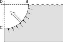
The key to this simple treatment is the resolution of the total force into horizontal and vertical components which we can then treat completely separately. Suppose we have the problem of calculating the total hydrostatic force acting on a large dam wall holding the water back in a reservoir.

We are looking for the single force F which represents the sum of all the little forces acting over all the dam wall. We can find this if we can calculate separately the horizontal and vertical forces acting on the wall due to the water. Let us begin with the vertical force.
Vertical force component
The vertical force caused by a static liquid which has a free surface open to the atmosphere results solely from gravity. In other words, the vertical force on this dam wall is simply the weight of the water pressing down on it. Clearly we only need to consider any water which is directly above any part of the wall, i.e. in the volume BCD, since gravity always acts vertically. Any water beyond BC only presses down on the bed of the reservoir, not on the wall.
Calculation of the volume BCD may seem complicated but in engineering the shapes usually have clearly defined profiles such as ellipses, parabolas or circles, which greatly simplify the problem.
Horizontal force component
The horizontal force component is what is left of the total force once we have removed the vertical component. It is therefore exactly the same as the force acting on a flat vertical wall of the same height and width. All we need to do then is calculate the force which would act on an imaginary vertical wall erected along BC, using the method developed in the previous section.
Total force (Figure 3.1.23)
Once the two components have been found it is a simple matter to calculate the single total force acting on the dam wall by recombining them:

It is also possible to calculate the direction of the total force to the horizontal or vertical:
Example 3.1.5
Fuel of relative density 0.8 is stored in a reservoir which is a tank of overall depth 5 m. One end of the tank is composed of two sections: a flat vertical plate of width 1.5 m and height 3 m, and below that is a curved plate that is a quadrant of a horizontal cylinder of radius 2 m. The two plates are welded together so that the curve bulges into the reservoir. If the tank is full to the brim, calculate the total liquid force on the curved plate.
First of all, we shall calculate the vertical force pressing down on the curve. This is the weight of fuel directly above the curve and so the first step is to work out the volume of this liquid. The curve protrudes into the tank by a distance of 2 m horizontally, i.e. its radius. Therefore the volume is the rectangular volume
minus the volume of the quadrant
Hence the total volume over the curve is 10.288 m3 and the weight pressing down is
Now we shall calculate the horizontal force acting on the curve. This is the force which would act on a flat vertical plate of the same width and height as the curved plate. Therefore this force is the product of the flat plate area and the mean pressure acting on it:
Note that the mean pressure is calculated half way down the flat plate that replaces the curved plate. The top of this is already at a depth of 3 m and so the total depth to the centroid works out to be 4 m.
We have now worked out the vertical and horizontal components of the hydrostatic thrust on the curved plate. It simply remains to combine them using Pythagoras’ theorem to find the resultant force F.
Upthrust
Sometimes it is necessary to calculate the total force on a curved surface which is arranged as in Figure 3.1.24.
In this case the small pressure forces all have an upwards component, unlike the example on the dam wall. It would seem that we can no longer use the simplification of calculating the vertical force component from the weight of liquid directly above the curved surface because, clearly, there is no liquid directly above to produce any weight.
However, suppose that the curve had not been there and so the end wall was simply a flat surface; the liquid would then occupy the extra volume BCD, and this liquid would be supported by the liquid underneath the curve BC. The liquid beneath BC must therefore be capable of exerting an upwards vertical force to balance the weight of the liquid that we have imagined to be filling the volume BCD. Hence the vertical force on the real curved surface BC is an upthrust whose magnitude is equal to the weight of the liquid which could be put into volume BCD.
This type of problem is therefore simply the inverse of the problem concerning the dam wall, and the calculation method is identical except that the vertical force will be upwards.
Archimedes’ principle
Imagine that we now have two surfaces joined back to back to form the hull of a ship (Figure 3.1.25).

The total force on the left side of the hull can be split up into a horizontal component and a vertical component, as can the total force on the right side. Each vertical component is an upthrust equal to the weight of liquid which could be put into half of the hull, up to the outside water level. Each horizontal component is the force which would act on a flat vertical wall with the same area as a side projection of the hull.
If we are interested in the total force on the whole ship, then the two horizontal components can be ignored because they are of equal magnitude and opposite direction, so they cancel each other out. The total force on the ship is therefore simply the sum of the two upthrusts, each one of which is equal to the weight of water which would fit into one half of the hull up to the waterline. In other words:
The upthrust on an immersed object is equal to the weight of liquid displaced.
This is known as Archimedes’ principle after the famous Greek philosopher who is said to have discovered it. It shows why large ships made out of very dense materials such as steel can nevertheless float if they are made large enough to displace a sufficient volume of water, contrary to the belief which was popularly held at one time that ships could only be made from materials such as wood which were less dense than water. It is worth noting that large crowds attended the launching of the first steel-hulled ship built by Brunel, fully expecting to witness a disaster caused by building it from a material which would not float.
It is also worth noting that for objects such as submarines which become completely submerged and can go to great depths, there is no increase in the upthrust with depth. Once a submarine is completely under the surface of the water, the upthrust does not get any bigger no matter how deep the vessel may dive since it only depends on the weight of water displaced.
Example 3.1.6
A crane is to lower a vertical cylindrical pillar, of diameter 1.2 m, into position on a plinth submerged in water. The pillar has a mass of 5 tonnes. What will be the tension experienced in the supporting cable when the lower end of the pillar is submerged to a depth of 2.3 m?
We need to calculate the weight of water displaced by the partly submerged pillar in order to find the upthrust and hence calculate the resultant tension in the support cable. The starting point is to calculate the volume of the pillar that is submerged. This is the volume of a cylinder of radius 0.6 m and length 2.3 m.

Hence the resultant tension in the cable with the pillar partly submerged is:
Buoyancy
This phenomenon of solid objects being able to float is part of a larger subject area known as buoyancy that includes examples of submerged objects which are not allowed to float but nevertheless experience a buoyancy force because of a surrounding liquid. It is one of the most important subjects studied by marine architects because it decides the stability of a ship. It can also become very complex, but it is worth taking a quick look at some of the main features.
The upthrust, or buoyancy force, is a summation of all the small upward forces acting on an immersed object. The usefulness of this summation lies in being able to think of the upthrust as a single force acting at a single point. The location of this single point must be the centre of gravity of the displaced liquid since only then can the upthrust fully cancel out the lost downward force. The point at which the buoyancy force acts is called the centre of buoyancy.
Stability of a floating body
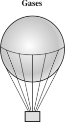
Have you ever wondered why the passenger basket on a hot air balloon is suspended underneath and not simply strapped to the top of the balloon? After all, most hot air balloons are used for sightseeing and a basket on the top would give much better views.
Consider the balloon shown in the left-hand diagram of Figure 3.1.26. The balloon floats because the hot air inside it is less dense than the cold air surrounding it, giving rise to a buoyancy force acting upwards through B. When this force equals the total weight of the balloon and basket, acting through the centre of gravity G, the balloon will float at a constant altitude. As the wind changes and the occupants of the basket move around, the balloon will rock through a small angleθ. Since the centre of buoyancy is higher than the centre of gravity, any angular displacement produces a turning moment which acts to restore the balloon to an upright position. Such an arrangement is said to be in stable equilibrium.

Now look at the bizarre case in the right-hand diagram. The buoyancy force again equals the weight, but here any angular displacement causes a turning moment which makes the basket topple over. The reason for this is that the centre of buoyancy B is below G. The situation is known as unstable equilibrium.
Something very similar applies to ships, but there are cases where stable equilibrium can be achieved even where the centre of buoyancy is below the centre of gravity. This occurs because the shape of the displaced water alters as the ship rocks and so the centre of buoyancy moves sideways in the same direction as the ship is leaning. Therefore the line of action of the buoyancy force also moves to the side of the ship which is further down in the water, and the buoyancy force tries to lift the ship back to the upright position.
Whether or not the restoring moment is enough to make the ship stable depends on the position of the point where the line of action of the buoyancy force crosses the centreline of the ship, known as the metacentre, M (Figure 3.1.27).

The distance between G and M is known as the metacentric height.
If M is above G then the metacentric height is positive and the ship is in stable equilibrium.
If G is above M then the metacentric height is negative and the ship is in unstable equilibrium. This is the situation which led to the sinking of King Henry VIII’s flagship, the Mary Rose, off Portsmouth. This had sailed successfully for a number of years and was just stable as it cast off on its fateful last voyage, even though an unusually large shipment of weapons and soldiers had raised the centre of gravity to danger level. Finally, when the soldiers crowded up onto deck for a last glimpse of land as the ship put out to sea, the centre of gravity rose so high that the first big wave they encountered away from the shelter of the harbour caused the ship to topple completely over.
Problems 3.1.1
(1) Find the height of a column of water which will produce a pressure equal to that of the atmosphere.
(2) Find the equivalent height to Problem 1 for a column of mercury.
(3) Referring to Figure 3.1.28, find:
(4) Find the difference in pressure head between two points on a horizontal pipe containing water if a mercury U-tube differential manometer gives a reading of 200 mm.
(5) What is the pressure difference between the two points in Problem 4?
(6) A mercury U-tube manometer indicates a reading of 135 mm when connected to a pipeline at points A and B, both at the same level but at some distance apart. If the pipe contains oil of density 800 kg/m3, what is the pressure difference between A and B?
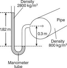
(7) A pipe contains water at a pressure of pA which is equivalent to a head of 150 mm of water (Figure 3.1.29). The pressure recorded on the manometer filled with liquid of density 2800 kg/m3 gives a scale reading of x on the right side, with the left-hand level on the zero of the scale. Calculate x.
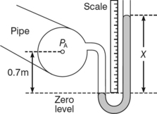
(8) If now the pressure pA increases to 2.0 kPa, find the new value of the height reading for the right-hand side of the manometer, assuming the scale is not moved.
(9) In a hydraulic jack a force is applied to a small piston to lift the load on a large piston. For a hydraulic jack which has a small piston of diameter 15 mm and a large piston of diameter 200 mm, determine the force required to lift a car of mass 1 tonne.
(10) A hydraulic testing machine is designed to exert a maximum load of 0.5 MN and utilizes a hand-operated pump. The hand lever itself has a ratio of 8:1 between the force output and the force exerted by the hand. The lever operates a piston of 20 mm diameter. The test head on the machine is operated by a hydraulic piston of 300 mm diameter. The two pistons are connected by a hydraulic pipe and the whole system contains a hydraulic oil. For maximum load, determine the pressure in the hydraulic oil and the force which must be applied to the lever by hand.
(11) A tank 1.5 m high, 1 m wide and 2.5 m long is filled with oil of relative density 0.9. Calculate the total force acting on:
(12) A rectangular lock gate 3.6 m wide can just withstand a resultant force of 1 MN. If the depth of water on the lower side is 3 m, to what depth can the water on the other side be allowed to rise?
(13) Calculate the hydrostatic thrust acting on the large side of a fish tank of length 2.8 m and height 1 m if the water is 85 cm deep.
If this side is hinged along its bottom edge so that it can be swung forward and down for cleaning, calculate the horizontal force experienced by a fastener at the top edge when it is holding the side in place and the tank is filled as above.
(14) Find the resultant hydrostatic force on two vertical plates used as gates to two separate pipes leading from a reservoir. In each case the centre of the plate is 1.2 m below the surface of the water:
(15) A square section, open irrigation channel of width 0.85 m is normally sealed at the outlet end by a vertical square flap which will swing downwards about an axis along the bottom edge of the channel when the hydrostatic torque is greater than 420 Nm. To what depth can the channel be filled before this flap opens and releases the water to the fields?
(16) A swimming pool is to have an underwater window consisting of a 10 m length quadrant, of radius 1 m, as shown in Figure 3.1.30. Calculate the magnitude and direction of the resultant hydrostatic thrust on the window.

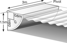
(17) A sluice gate (Figure 3.1.31) consists of a quadrant of a cylinder of radius 1.5 m, pivoted so that it can be rotated upwards to open. Its centre of gravity is at G, its mass is 6000 kg and its length (into the paper) is 3 m. Calculate:
(18) A 10 m deep dolphin pool is to be fitted with an observation tunnel on the horizontal base of the pool so that visitors can see the dolphins from underneath (Figure 3.1.32). The tunnel is made from plate glass panels of radius 2.4 m and width 0.9 m. If the pool is filled with seawater of relative density 1.06, calculate the magnitude and direction of the hydrostatic thrust on one panel.

(19) A cruise liner is to be fitted with a hemispherical glass observation window, which will be let into the side of the hull below the waterline. The radius of the hemisphere will be 2.6 m and its top edge will be 3 m below the water surface. If the sea water has a density of 1058 kg/m3, calculate the horizontal and vertical hydrostatic forces acting on the window.
(20) A tank of water of total mass 6 kg stands on a set of scales. An iron block of mass 2.8 kg and relative density 7.5 is lowered into the water on the end of a fine wire hanging from a spring balance. When the block is completely immersed in the water, what will be the reading on the scales and on the balance?
3.2 Hydrodynamics – fluids in motion
This section deals with hydrodynamics – fluids in motion. There are two important concepts that apply here: conservation of energy and Newton’s second law. Both of these will be familiar to the reader from earlier studies and so the treatment here concentrates on their application to fluids. The section starts with a detailed description of the types of fluid flow in order to build an understanding of the way in which energy can be lost by a fluid to its surroundings.
Fluid flow
Much of fluid mechanics for engineers is concerned with flowing liquids: pumped flow of fuel and lubricants, flow of water through generators, etc. To understand how we can analyse these flows we must first be able to recognize different types of flow, and fortunately there are only two important types. Flow of a fluid is generally either streamlined or turbulent. The key to understanding the difference lies in remembering that the fluid is made up of molecules and we can look in detail at the way in which they move in addition to looking on a large scale at the way in which the fluid moves as a whole.
Streamlined flow (Figure 3.2.1) is when a particle in the liquid can be traced and shown to move along a smooth line in the direction of flow. Suppose we could take a series of very high-speed photographs of a single particle in the fluid and build up a multiple exposure record of what the particle does. In streamlined flow we would see that the particle followed exactly the line of flow of the liquid, as in this illustration of a particle flowing along in a tube. In this case the line of flow of the fluid is known as a streamline because the individual particles stream along it.

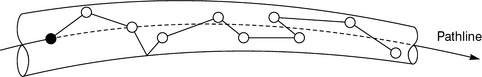
Turbulent flow is when the individual particles do not follow any regular path but their overall motion gives rise to the liquid flow. The particles are clearly being stirred around in the fluid and undergo many collisions with their colleagues. As a result they are knocked sideways from the direction of flow, and sometimes may even travel against the direction of flow for a short distance. Nevertheless the liquid in the example shown below is still flowing in the same direction as that in the example above and so we know that the particles must ultimately travel along the tube from left to right. The route taken by the fluid at any point is called a pathline. In the example in Figure 3.2.2 the pathline looks identical to the streamline in Figure 3.2.1, but the difference is that the individual particles do not follow it.
The difference between the two extreme types of flow is rather like the difference between taking a dog for a walk on a lead and off a lead. When the dog is on the lead it follows exactly the same route as its owner but displaced slightly to one side, just like two adjacent molecules in laminar or streamlined flow. When the dog is let off the lead on a country path it will race around exploring its surroundings, sometimes going back down the path for a short distance, but overall it follows the same route as its owner. This is like turbulent flow.
Since these two diagrams look so similar and we can only tell the detailed molecular pictures apart with the aid of a high-speed camera connected to a high power microscope, how can we predict when we will get one kind of flow and not the other?
Osborne Reynolds
This question was the big thing on the mind of a Manchester scientist called Osborne Reynolds who became involved in the development work for one of the greatest Victorian engineering projects of the late nineteenth century, Tower Bridge in London. At the time this was conceived as an enormous advance in engineering terms since it involved the bridge’s roadway being divided into two halves which could be lifted like drawbridges at the entrance to a castle. The bearings required for supporting the roadways as they were raised when a ship needed to pass into the Pool of London were many times larger than any that had been constructed up to that point for applications such as railway locomotives. Suddenly engineers realized that they had no real idea how fluid bearings worked in detail, largely because they did not understand in detail how fluids flowed, and so nobody could design the new giant bearings. This is where Reynolds came to the rescue, eventually producing a long equation which described how fluid bearings can generate enough pressure to keep the metal surfaces apart. He began, however, by carrying out some simple experiments on fluid flow.
The apparatus he used was something like that shown in Figure 3.2.3.
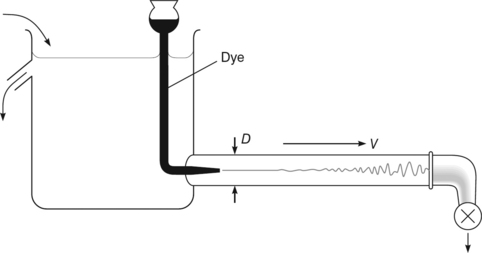
Reynolds filled the large tank with a range of liquids of different densities and viscosities and allowed them to flow at different rates by adjusting the valve at the end of the glass tube. He also could change the glass tube for others of different diameters. The clever part was to mark the flow by injecting a dye into the entrance of the glass tube via a funnel connected to a fine jet.
Reynolds found that if the liquid velocity was low then the fine stream of dye remained undisturbed all the way along the glass tube. He had discovered streamlined flow (Figure 3.2.4), because the fact that the dye did not get mixed up showed that the fluid itself was flowing very smoothly. This type of flow is also known as laminar flow, from a Latin origin which means that it is in distinct layers. Reynolds obtained particularly good results when the tube was of small diameter and the liquid was very viscous.
If the liquid velocity was high, because the valve was opened wide, the dye was stirred up almost as soon as it left the jet on the end of the funnel. This effect was strongest when the tube diameter was large and the liquid had a low viscosity. This was turbulent flow (Figure 3.2.5) and the mixing was caused by the fact that the molecules themselves were flowing along in a very agitated manner.
In between these two extremes the transition from smooth dye streams to stirred-up dye took place at different lengths along the glass tube as one type of fluid flow gave way to another. Reynolds managed to make sense of the different combinations of velocities, tube diameters, viscosities and even liquid densities (although density does not generally vary much from one liquid to another) by coming up with the idea of a dimensionless quantity which determined what kind of flow could be expected. This is now known as the Reynolds number, given by:
where:
Streamlined flow occurs at low Reynolds numbers, while turbulent flow occurs at high Reynolds numbers. The transition from streamlined to turbulent flow occurs at a Reynolds number of about 2000. This transition can be illustrated by looking at the results of measuring the differential pressure applied to the two ends of a pipe to produce an increasing flow rate (like plotting voltage against current for an electrical circuit) (Figure 3.2.6).

Within the linear, streamlined region at low velocities the flow rate can be doubled by doubling the pressure applied. However, within the turbulent region the flow rate can only be doubled by quadrupling the pressure. This gives us one of the big conclusions to be drawn from Reynolds’ work:
Turbulent flow requires large applied pressures and that can lead to high energy losses.
This is a big generalization and sometimes turbulent flow is an advantage (e.g. dishwashers use high velocity jets of water to create turbulent flow because the jets of swirling liquid achieve a better cleaning action than a smooth jet of streamlined flow). Nevertheless it is usually advantageous to try to achieve as smooth a flow pattern as possible. Hence there is great emphasis on ‘streamlining’ of cars, for example. Different definitions of Reynolds number are required to overcome the fact that airflow around a car is not the same as flow in a tube, but the principle is the same.
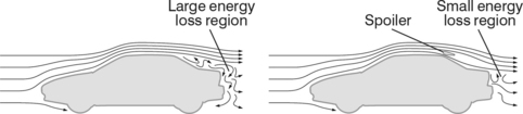
Figure 3.2.7 shows the idea behind the spoilers which are attached to the tailgate or boot of some cars.
Continuity
Having studied the work of Reynolds we are now ready to apply some of our knowledge to the flow of real liquids along pipes since this is the situation which is most important to mechanical engineers. For most practical applications the flow of liquids along pipes is turbulent because the combination of values which have to be put into Reynolds number leads to it being well over 2000. For example, consider water flowing along a pipe in your home. The density of water is 1000 kg/m3 and its dynamic viscosity is approximately 0.001 pascal seconds, as shown in the table of fluid properties in Section 3.1 (page 127). Together these two terms account for a total of one million in Reynolds number and so the velocity and diameter would need to be very small to bring the final value down to less than 2000. Typically the water pipe diameter in your home would be 12 mm (i.e. 0.012 m for substitution into any calculation) and the water would leave a fully opened tap at a speed of about 1 m/s. The final value for Reynolds number in this situation is therefore about 12 000 and so the flow is very turbulent. This means that the liquid is stirred around as it flows along a pipe and so any differences in velocity from one side of the pipe to the other are eliminated. Hence all the fluid moves along the pipe with the same mean velocity, except for a tiny fraction around the edge which is slowed down by contact with the pipe wall.
Figure 3.2.8 shows what happens to the liquid in a pipe during a time span of 1 second.

If all the liquid is travelling down the pipe at a velocity of v metres/second then in the time span of 1 second the chosen cross-section in the liquid will move by a distance of v metres along the pipe. Therefore the volume of liquid which has passed the starting position is the volume of the cylinder which has been shaded. This volume is end area × length, which equals A × v. Since this is the volume of liquid which has passed an arbitrary point in 1 second, the volume flow rate of liquid along the pipe is given by:
Suppose now that the pipe considered above is connected to a smaller diameter pipe by a tapered section, as shown in Figure 3.2.9.
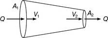
The volume flow rate Q must stay the same all the way along the pipes, even though the velocities v1 and v2 will be different, because whatever enters the pipe at one end must leave it at the other end at the same rate otherwise the pipe would inflate and eventually explode. Therefore the flow rate at the entry, Q = A1v1, must equal the flow rate at the other end, Q = A2v2.
This is known as the continuity equation and is very important in calculations involving pipe flow. It is part of a much more universal principle known as the continuity law, which is to do with the fact that fluids cannot be torn apart like a solid.
Sometimes it is necessary to work out the velocities and flow rates in a network of pipes, such as the case where a number of pumps are forcing oil into a large undersea pipeline which subsequently splits into several branches at a tanker loading terminal. This situation can be analysed using the continuity law provided it is remembered that what goes in at one end, from all the different inlets, must come out at the same rate at the other end, through all its branches.
Although we deliberately stated at the start of this section on continuity that we were looking at turbulent flow, this equation applies equally well to laminar flow so long as we remember to use the mean or average velocity. This is because the velocity variation across a pipe containing laminar or streamlined flow is very wide. The relationship between the mean velocity and the maximum velocity for laminar flow will be developed in the next section.
Example 3.2.2
A liquid is flowing along a tapering pipe at a volume flow rate of 15 m3/min. The cross-sectional area of the pipe at the start is 0.05 m2 and this reduces to 0.02 m2 at the outlet. Calculate the flow velocity at the inlet and outlet to the pipe.
This is an example of the use of the continuity law represented in Equation (3.2.3). We must remember to convert the volume flow rate to cubic metres per second from cubic metres per minute.

Laminar flow
Before we can consider flow of fluids in much more detail, we must take a closer look at the property of fluids known as viscosity. We have already met viscosity as one of the quantities in Reynolds equation where we have used it to represent the ‘oiliness’ of a fluid. Fluids such as oils and syrup that flow sluggishly have a high value of viscosity, while thin, watery fluids have a low viscosity. The concept of viscosity is generally credited to Newton who studied it experimentally and came up with an equation which essentially defines viscosity. In fact Newton was not directly interested in the flow of liquids; his life’s work was devoted to the study of the stars and planets, eventually coming up with the idea of gravity. He became involved with the study of viscosity almost by chance as a means of explaining the small variations in speed of the planets when they are closest to one of their neighbouring planets. For example, he had studied the fact that the earth temporarily moves faster along its orbit when its quicker neighbour, Venus, overtakes it from time to time. As a result of Newton’s later work we now know that this effect is caused by the gravitational attraction between the two planets but initially Newton thought that it was due to viscous drag in the celestial fluid or ether that was held to fill the universe. When Venus passed the earth it would shear this fluid in the relatively small gap between the two planets and there would be a resistance or drag force which would act to slow Venus down while speeding up the earth. Newton pursued this theory to the point of tabletop experiments with liquids and plates and produced an equation which basically describes and defines viscosity, before discarding the idea in favour of gravity.
The equation that Newton developed to define the viscosity of a fluid is:
In its simplest form this can be applied to two flat plates, one moving and one stationary, in the following equation:
Here the force F applied to one of the plates, each of area A and separated by a gap of width h filled with fluid of viscosityμ, produces a difference in velocity of u. The viscosity is correctly known as the dynamic viscosity and has the units of Pascal seconds (Pa s). These are identical to N s/m2 and kg/m/s.
For the case where these two plates are adjacent lamina or layers:
We have replaced the term u/h with something called the velocity gradient which will allow us later to apply Newton’s equation to situations where the velocity does not change evenly across a gap.
We can apply this to pipe flow if we now wrap the lamina into cylinders.
Laminar flow in pipes (Figure 3.2.10)
We said earlier that most fluid flow applications of interest to mechanical engineers involve turbulent flow, but there are some increasingly important examples of laminar flow where the pipe diameter is small and the liquid is very viscous. The field of medical engineering has many such examples, such as the flow of viscous blood along the small diameter tubes of a kidney dialysis machine. It is therefore necessary for us to study this kind of pipe flow so that we may be able to calculate the pumping pressure required to operate this type of device.

Consider flow at a volume flow rate Q m3/s along a pipe of radius R and length L. The liquid viscosity is μand a pressure drop of P is required across the ends of the pipe to produce the flow. Let us look at the forces on the cylindrical core of the liquid in the pipe, up to a radius of r.
If we take the outlet pressure as 0 and the inlet pressure as P then the force pushing the core to the right, the pressure force, is given by
The force resisting this movement is the viscous drag around the cylindrical surface of the core. Using Newton’s defining equation for viscosity, Equation (3.2.4),

For steady flow these forces must be equal and opposite,
So the velocity gradient is
This is negative because v is a maximum at the centre and decreases with radius.
We need to relate the pressure to the flow rate Q and the first step is to find the velocity v at any radius r by integration.

To evaluate the constant C we note that the liquid is at rest (v = 0) at the pipe wall (r = R). Even for liquids which are not sticky or highly viscous, all the experimental evidence points to the fact that the last layer of molecules close to the walls fastens on so tightly that it does not slip (Figure 3.2.11).

Therefore
This is the equation of a parabola so the average or mean velocity equals half the maximum velocity, which is on the central axis.
Now volume flow rate is Q = Vmean × area.
This is the continuity equation and up to now we have only applied it to turbulent flow where all the liquid flows at the same velocity and we do not have to think of a mean. So
Finally
This is called Poiseuille’s law after the French scientist and engineer who first described it and this type of flow is known as Poiseuille flow.
Note that this is analogous to Ohm’s law with flow rate Q equivalent to current I, pressure drop P equivalent to voltage E and the term
representing fluid resistance Ω, equivalent to resistance R.
Hence Ohm’s law E = IR becomes P = QΩ when applied to viscous flow along pipes. This can be very useful when analysing laminar flow through networks of pipes. For example, the combined fluid resistance of two different diameter pipes in parallel and both fed with the same liquid at the same pressure can be found just like finding the resistance of two electrical resistors in parallel.
Example 3.2.3
A pipe of length 10 m and diameter 5 mm is connected in series to a pipe of length 8 m and diameter 3 mm. A pressure drop of 120 kPa is recorded across the pipe combination when an oil of viscosity 0.15 Pa s flows through it. Calculate the flow rate.
First we must calculate the two fluid resistances, one for each section of the pipe.

Total resistance = 70.139 × 10¹⁰ Pa s/m3

Examples of laminar flow in engineering
We have already touched on one example of laminar flow in pipes which is highly relevant to engineering but it is worthwhile looking at some others just to emphasize that, although turbulent flow is the more important, there are many instances where knowledge of laminar flow is necessary.
One example from mainstream mechanical engineering is the dashpot. This is a device which is used to damp out any mechanical vibration or to cushion an impact. A piston is pushed into a close-fitting cylinder containing oil, causing the oil to flow back along the gap between the piston and the cylinder wall. As the gap is small and the oil has a high viscosity, the flow is laminar and the pressure drop can be predicted using an adaptation of Poiseuille’s law.
A second example which is more forward looking is from the field of micro-fluidics. Silicon chip technology has advanced to the point where scientists can build a small patch which could be stuck on a diabetic’s arm to provide just the right amount of insulin throughout the day. It works by drawing a tiny amount of blood from the arm with a miniature pump, analysing it to determine what dose of insulin is required and then pumping the dosed blood back into the arm. The size of the flow channels is so small, a few tens of microns across, that the flow is very laminar and therefore so smooth that engineers have had to go to great lengths to ensure effective mixing of the insulin with the blood.
Conservation of energy
Probably the most important aspect of engineering is the energy associated with any application. We are all painfully aware of the cost of energy, in environmental terms as well as in simple economic terms. We therefore now need to consider how to keep account of the energy associated with a flowing liquid. The principle that applies here is the law of conservation of energy which states that energy can neither be created nor destroyed, only transferred from one form to another. You have probably met this before, and so we have a fairly straightforward task in applying it to the flow of liquids along pipes. If we can calculate the energy of a flowing liquid at the start of a pipe system, then we know that the same total of energy must apply at the end of the system even though the values for each form of energy may have altered. The only problem is that we do not know at the moment how to calculate the energy associated with a flowing liquid or even how many types of energy we need to consider. We must begin this calculation therefore by examining the different forms of energy that a flowing liquid can have (Figure 3.2.12).

If we ignore chemical energy and thermal energy for the purposes of flow calculations, then we are left with potential energy due to height, potential energy due to pressure and kinetic energy due to the motion.
In Figure 3.2.12 adding up all three forms of energy at point 1 for a small volume of liquid of mass m:
Potential energy due to height is calculated with reference to some datum level, such as the ground, in the same way as for a solid.
Potential energy due to pressure is a calculation of the fact that the mass m could rise even higher if the pipe were to spring a leak at point 1. It would rise by a height of h1 equal to the height of the liquid in a manometer tube placed at point 1, where h1 is given by h1 = p1/ρ g. Therefore the energy due to the pressure is again calculated like the height energy of a solid.
Note that the height h1 is best referred to as a pressure head in order to distinguish it from the physical height z1 of the pipe at this point.
Kinetic energy is calculated in the same way as for a solid.
Therefore the total energy of the mass m at point 1 is given by
Similarly the energy of the same mass at point 2 is given by
From the principle of conservation of energy we know that these two values of the total energy must be the same, provided that we can ignore any losses due to friction against the pipe wall or within the liquid. Therefore if we cancel the m and divide through by g, we produce the following equation:
This is known as Bernoulli’s equation after the French scientist who developed it and is the fundamental equation of hydrodynamics. The dimensions of each of the three terms are length and therefore they all have units of metres. For this reason the third term, representing kinetic energy, is often referred to as the velocity head, in order to use the familiar concept of head which already appears as the second term on both sides of the equation. The three terms on each side of the equation, added together, are sometimes known as the total head. A second advantage to dividing by the mass m and eliminating it from the equation is that we no longer have to face the problem that it would be very difficult to keep track of that fixed mass of liquid as it flowed along the pipe. Turbulent flow and laminar flow would both make the mass spread out very rapidly after the starting point.
Bernoulli’s equation describes the fact that the total energy in an ideal flowing liquid stays constant between two points. It is very much a practical engineering equation and for this reason it is commonly reduced to the form given here where all the terms are measured in metres. A pipeline designer, for example, could use it to keep track of how the pressure head would change along a pipe system as it followed the local terrain over hill and valley, without any need to ever work in joules, the true units of energy.
When carrying out calculations on Bernoulli’s equation it is sometimes useful to use the substitution h = p/ρ g to change from head to pressure, and it is often useful to use the substitution v = Q/A because the volume flow rate is the most common way of describing the liquid’s speed.
An example of the use of Bernoulli’s equation is given later in Example 3.2.5.
Venturi principle
Bernoulli’s equation can seem very daunting at first sight, but it is worthwhile remembering that it is simply the familiar conservation of energy principle. Therefore it is not always necessary to put numbers into the equation in order to predict what will happen in a given flow situation. One of the most useful applications in this respect is the behaviour of the fluid pressure when the fluid, either liquid or gas, is made to go through a constriction.
Consider what happens in Figures 3.2.13 and 3.2.14
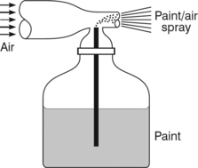

In both cases the fluid, air, is pushed through a narrower diameter pipe by the high pressure in the large inlet pipe. The velocity in the narrow pipe is increased according to the relationship v = Q/A since the volume flow rate Q must stay constant. Hence the kinetic energy term v2/2g in Bernoulli’s equation is greatly increased, and so the pressure head term h or p/ρ g must be much reduced if we can ignore the change in physical height over such a small device. The result is that a very low pressure is observed at the narrow pipe, which can be used to suck paint in through a side pipe in the case of the spray gun in Figure 3.2.13, or petrol in the case of the carburettor in Figure 3.2.14. This effect is known as the Venturi principle after the Italian scientist and engineer who discovered it.
Measurement of fluid flow
Fluid mechanics for the mechanical engineer is largely concerned with transporting liquid from one place to another and therefore it is important that we have an understanding of some of the ways of measuring flow. There are many flow measurement methods, some of which can be used for measuring volume flow rates, others which can be used for measuring flow velocity, and yet others which can be used to measure both. We shall limit ourselves to analysis of one example of a simple flow rate device and one example of a velocity device.
Measurement of volume flow rate – the Venturi meter
In the treatment of Bernoulli’s equation we found that changing the velocity of a fluid through a change of cross-section leads to a change in the pressure as the total head remains constant. In the Venturi effect the large increase in velocity through a constriction causes a marked reduction in pressure, with the size of this reduction depending on the size of the velocity increase and therefore on the degree of constriction. In other words, if we made a device which forced liquid through a constriction and we measured the pressure head reduction at the constriction, then we could use this measurement to calculate the velocity or the flow rate from Bernoulli’s equation.
Such a device is called a Venturi meter since it relies on the Venturi effect. In principle the constriction could be an abrupt change of cross-section, but it is better to use a more gradual constriction and an even more gradual return to the full flow area following the constriction. This leads to the formation of fewer eddies and smaller areas of recirculating flow. As we shall see later, this leads to less loss of energy in the form of frictional heat and so the device creates less of a load to the pump producing the flow. A typical Venturi meter is shown in Figure 3.2.15.

The inlet cone has a half angle of about 45° to produce a flow pattern which is almost free of recirculation. Making the cone shallower would produce little extra benefit while making the device unnecessarily long.
The diffuser has a half angle of about 8° since any larger angle leads to separation of the flow pattern from the walls, resulting in the formation of a jet of liquid along the centreline, surrounded by recirculation zones.
The throat is a carefully machined cylindrical section with a smaller diameter giving an area reduction of about 60%.
Measurement of the drop in pressure at the throat can be made using any type of pressure sensing device but, for simplicity, we shall consider the manometer tubes shown. The holes for the manometer tubes – the pressure taps – must be drilled into the meter carefully so that they are accurately perpendicular to the flow and free of any burrs.
Analysis of the Venturi meter
The starting point for the analysis is Bernoulli’s equation:
Since the meter is being used in a horizontal position, which is the usual case, the two values of height z are identical and we can cancel them from the equation.
The constriction will cause some non-uniformity in the velocity of the liquid even though we have gone to the trouble of making the change in cross-section gradual. Therefore we cannot really hope to calculate the velocity accurately. Nevertheless we can think in terms of an average or mean velocity defined by the familiar expression:
Therefore, remembering that the volume flow rate Q does not alter along the pipe:
We are trying to get an expression for the flow rate Q since that is what the instrument is used to measure, so we need to gather all the terms with it onto the left-hand side:

Since h1 > h2 it makes sense to reverse the order in the first set of brackets, compensating by reversing the order in the second set as well:
Finally we have:
This expression tells us the volume flow rate if we can assume that Bernoulli’s equation can be applied without any consideration of head loss, or energy loss, in the device. In practice there will always be losses of energy, and head, no matter how well we have guided the flow through the constriction. We could experimentally measure a head loss and use this in a modified form of Bernoulli’s equation, but it is customary to stick with the analysis carried out above and make a final correction at the end.
Any loss of head will lead to the drop in heights of manometer levels across the meter being bigger than it should be ideally. Therefore the calculated flow rate will be too large and so it must be corrected by applying some factor which makes it smaller. This factor is known as the discharge coefficient CD and is defined by:
In a well-manufactured Venturi meter the energy losses are very small and so CD is very close to 1 (usually about 0.97).
In some situations it would not matter if the energy losses caused by the flow measuring device were considerably higher. For example, if you wanted to measure the flow rate of water entering a factory then even a considerable energy loss caused by the measurement would only result in the pumps at the local water pumping station having to work a little harder; there would be no disadvantage as far as the factory was concerned. In these circumstances it is not necessary to go to the trouble of having a carefully machined, highly polished Venturi meter, particularly since they are complicated to install. Instead it is sufficient just to insert an orifice plate at any convenient joint in the pipe, producing a device known as an Orifice meter (Figure 3.2.16). The orifice plate is rather like a large washer with the central hole, or orifice, having the same sort of area as the throat in the Venturi meter.
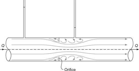
The liquid flow takes up a very similar pattern to that in the Venturi meter, but with the addition of large areas of recirculation. In particular the flow emerging from the orifice continues to occupy a small cross-section for quite some distance downstream, leading to a kind of throat. The analysis is therefore identical to that for the Venturi meter, but the value of the discharge coefficient CD is much smaller (typically about 0.6). Since there is not really a throat, it is difficult to specify exactly where the downstream pressure tapping should be located to get the most reliable reading, but guidelines for this are given in a British Standard.
Measurement of velocity – the Pitot-static tube
Generally it is the volume flow rate which is the most important quantity to be measured and from this it is possible to calculate a mean flow velocity across the full flow area, but in some cases it is also important to know the velocity at a point. A good example of this is in a river where it is essential for the captain of a boat to know what strength of current to expect at any given distance from the bank; calculating a mean velocity from the volume flow rate would not be much help even if it were possible to measure the exact flow area over an uneven river bed.
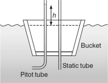
It was exactly this problem which led to one of the most common velocity measurement devices. A French engineer called Pitot was given the task of measuring the flow of the River Seine around Paris and found that a quick and reliable method could be developed from some of the principles we have already met in the treatment of Bernoulli’s equation. Figure 3.2.17 shows the early form of Pitot’s device.

The horizontal part of the glass tube is pointed upstream to face the oncoming liquid. The liquid is therefore forced into the tube by the current so that the level rises above the river level (if the glass tube was simply a straight, vertical tube then the water would enter and rise until it reached the same level as the surrounding river). Once the water has reached this higher level it comes to rest.
What is happening here is that the velocity head (kinetic energy) of the flowing water is being converted to height (potential energy) inside the tube as the water comes to rest. The excess height of the column of water above the river level is therefore equal to the velocity head of the flowing water:
Therefore the velocity measured by a Pitot tube is given by:
In practice Pitot found it difficult to note the level of the water in the glass tube compared to the level of the surrounding water because of the disturbances on the surface of the river. He quickly came up with the practical improvement of using a straight second tube (known as a static tube) to measure the river level because the capillary action in the narrow tube damped down the fluctuations (Figure 3.2.18).
The Pitot-static tube is still widely used today, most notably as the speed measurement device on aircraft (Figure 3.2.19).
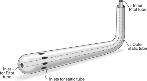
The two tubes are now combined to make them co-axial for the purposes of ‘streamlining’, and the pressure difference would be measured by an electronic transducer, but essentially the device is the same as Pitot’s original invention. Because the Pitot tube and the static tube are united, the device is called a Pitot-static tube.
Example 3.2.4
A Pitot-static tube is being used to measure the flow velocity of liquid along a pipe. Calculate this velocity when the heights of the liquid in the Pitot tube and the static tube are 450 mm and 321 mm respectively.
The first thing to do is calculate the manometric head difference, i.e. the difference in reading between the two tubes.
Then use Equation (3.2.7),
Losses of energy in real fluids
So far we have looked at the application of the familiar ‘conservation of energy’ principle to liquids flowing along pipes and developed Bernoulli’s equation for an ideal liquid flowing along an ideal pipe. Since energy can neither be created nor destroyed, it follows that the three forms of energy associated with flowing liquids – height energy, pressure energy and kinetic energy – must add up to a constant amount even though individually they may vary. We have used this concept to understand the working of a Venturi meter and recognized that a practical device must somehow take into account the loss of energy from the fluid in the form of heat due to friction. This was quite simple for the Venturi meter as the loss of energy is small but we must now consider how we can take into account any losses in energy, in the form of heat, caused by friction in a more general way. These losses can arise in many ways but they are all caused by friction within the liquid or friction between the liquid and the components of the piping system. The big problem is how to include what is essentially a thermal effect into a picture of liquid energy which deliberately sets out to exclude any mention of thermal energy.
Modified Bernoulli’s equation
Bernoulli’s equation, as developed previously, may be stated in the following form:
All the three terms on each side of Bernoulli’s equation have dimensions of length and are therefore expressed in metres. For this reason the total value of the three terms on the left-hand side of the equation is known as the initial total head in just the same way as we used the word head to describe the height h associated with any pressure p through the expression
Similarly the right-hand side of the equation is known as the final total head. Bernoulli’s equation for an ideal situation may also be expressed in words as:
What happens when there is a loss of energy due to friction with a real fluid flowing along a real pipe is that the final total head is smaller than the initial total head. The loss of energy, as heat generated by the friction and dissipated through the liquid and the pipe wall to the surroundings, can therefore be expressed as a loss of head. Note that we are not destroying this energy, it is just being transformed into thermal energy that cannot be recovered into a useful form again. As far as the engineer in charge of the installation is concerned this represents a definite loss which needs to be calculated even if it cannot be reduced any further.
What happens in practice is that manufacturers of pipe system components, such as valves or couplings, will measure this loss of head for all their products over a wide range of sizes and flow rates. They will then publish this data and make it available to the major users of the components. Provided that the sum of the head losses of all the components in a proposed pipe system remains small compared to the total initial head (say about 10%) then it can be incorporated into a modified Bernoulli’s equation as follows:
With this equation it is now possible to calculate the outlet velocity or pressure in a pipe, based on the entry conditions and knowledge of the energy losses expressed as a head loss in metres. Once again we see the usefulness of working in metres since engineers can quickly develop a feel for what head loss might be expected for any type of fitting and how it could be compensated. This would be extremely difficult to do if working in conventional energy units.
Example 3.2.5
Water is flowing downwards along a pipe at a rate of 0.8 m3/s frompoint A, where the pipe has a diameter of 1.2 m, to point B, where the diameter is 0.6 m. Point B is lower than point A by 3.3 m. The pipe and fittings give rise to a head loss of 0.8 m. Calculate the pressure at point B if the pressure at point A is 75 kPa (Figure 3.2.20).

Since the information in the question gives the flow rate Q rather than the velocities, we shall use the substitution
Therefore the modified Bernoulli’s equation becomes:
The absolute heights of point A and point B do not matter, it is only the relative difference in heights which is important. Therefore we can put z1 = 3.3 m and z2 = 0

Therefore:
The cause of energy losses
Earlier we looked at the way that liquids flow along pipes and we showed that almost all practical cases involved turbulent flow where the liquid molecules continually collide with each other and with the walls. It is the collisions with the walls which transfer energy from the liquid to the surroundings; the molecules hit a roughness point on the wall and lose some of their kinetic energy as a tiny amount of localized heating of the material in the pipe wall.
The molecules therefore bounce off the walls with slightly lower velocity, but this is rapidly restored to its original value in collisions with other molecules. If this velocity remained lower following a collision then the liquid would not flow along the pipe at the proper rate. This cannot happen since it would violate the continuity law, which states that the flow rate must remain constant. In fact the energy to keep the molecules moving at their original speed following a collision with the wall comes from the pressure energy, which is why the effect of friction appears as a loss of head.
Losses in pipe fittings
Let us look at a typical pipe fitting to see where the energy loss arises (see Figure 3.2.21).
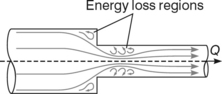
The sudden contraction of the flow caused by joining two pipes of different diameters gives rise to regions of recirculating flow or eddies. The liquid which enters these regions is trapped and becomes separated from the rest of the flow. It goes round and round, repeatedly hitting the pipe walls and losing kinetic energy, only to be restored to its original speed by robbing the bulk flow of some of its pressure energy. The energy is dissipated as heat through the pipe walls. If the overall pressure drop was critical and the head loss needed to be kept to a minimum, then a purpose-built pipe fitting could be designed to connect the two pipes with much less recirculation. Essentially this would round off the sharp corners (Figure 3.2.22).

Since it is kinetic energy which is lost in the collisions which are a feature of recirculating eddies, it follows that faster liquids will lose more energy than slower liquids in the same situation. In extensive experiments it has been found that the energy loss in fact depends on the overall kinetic energy of the liquid as it meets the obstruction. The proportion of the kinetic energy that is lost is approximately a constant for any given shape of obstruction, such as a valve or a pipe fitting, irrespective of the size.
For the purposes of calculations involving Bernoulli’s equation it is convenient to work in terms of the velocity head (i.e. the third term v2/2 g in Bernoulli’s equation) when considering kinetic energy. Therefore a head loss for a particular type of pipe fitting is usually expressed as:

Some typical values of k are shown below, but it must be remembered that they are only approximate.
Turbulent flow in pipes – frictional losses
One of the basic things that engineers need to know when designing and building anything involving flow of fluids along pipes is the amount of energy lost due to friction for a given pipe system at a given flow rate. We have just looked at the losses in individual fittings as these are of most importance in a short pipe system, such as would be found in the fuel or hydraulic system in a car. Increasingly, however, mechanical engineers are becoming involved in the design of much larger pipe systems such as would be found in a chemical plant or an oil pipeline. For these pipe lengths the head loss due to friction becomes appreciable for the pipes themselves, even though modern pipes are seemingly very smooth.
The energy loss due to friction appears as a loss of pressure (remember pressure and kinetic energy are the two important forms of energy for flow along a horizontal pipe – loss of kinetic energy becomes transformed into a loss of pressure). Therefore if we use simple manometers to record the pressure head along a pipeline then we observe a gradual loss of head. The slope of the manometer levels is known as the hydraulic gradient (Figure 3.2.23).

The head reading on the manometers can be held constant if the pipe itself goes downhill with a slope equal to the hydraulic gradient. Of course we do not really need to install manometer tubes every few metres; we can simply calculate the total head at any point and keep track of its gradual reduction mathematically.
There is no way of predicting the loss of head completely analytically and so we rely on an empirical law based on the results of a large number of experiments carried out by a French engineer Henri Darcy (or d’Arcy) in the nineteenth century. His results for turbulent flow were summed up as follows:
where:
Intuitively we can see where each of these terms comes from in the overall equation, as follows:
• The frictional head loss clearly depends on the length of the pipe, L, as we would expect a pipe that is twice as long to have a head loss that is also twice as great.
• Head loss decreases with increasing pipe diameter because a smaller proportion of the liquid comes into contact with the pipe wall.
• Friction arises from loss of kinetic energy and so the expression must have velocity head (V2/2g) in it (which is why we do not cancel the 2 and the 4).
• Head loss also depends on the resistance offered by the roughness of the pipe wall, as represented by the friction factor f.
The friction factor is generally quoted by a pipe manufacturer. It depends on the material and the type of production process (both of which affect the roughness), on the diameter and the flow velocity, and on the amount of turbulence (Reynolds number).
D’Arcy’s equation was used successfully for almost 100 years, relying on values of the friction coefficient f that were found experimentally for the very few types of pipes that were available and mostly for gravity feed systems. Once pumping stations and standardized pipes came into common use, however, a more accurate estimate of head loss at the much higher flow rates was required. It became apparent that the friction coefficient f varied quite considerably with type of pipe, diameter, flow rate, type of liquid, etc. The problem was solved by an American engineer called Moody who carried out a vast number of experiments on as many combinations of pipes and liquids as he could find. He assembled all the experimental data into a special chart, now called a Moody chart, as shown in Figure 3.2.24.

This has a series of lines on a double logarithmic scale. Each line corresponds to a pipe of a given ‘relative roughness’ and is drawn on axes which represent friction factor and Reynolds number. To understand the chart we must first look at the pipe roughness as this is the parameter which gives rise to most of the friction.
The roughness on the inside of the pipe is firstly expressed as an ‘equivalent height’ of roughness. This is an averaging process which imagines the actual randomly scattered roughness points being replaced by a series of identical rough points, all of one height, which produce the same effect. The pipe manufacturers will produce this information using a surface measurement probe linked to a computer. This equivalent roughness height K is then divided by the pipe diameter d to give the relative roughness, K/d, plotted down the right-hand edge of the chart. Note that the relative roughness has no units, it is simply a ratio. Therefore the whole chart is dimensionless since the axes themselves are friction factor and Reynolds number, neither of which has units.
To use the chart, calculate the relative roughness if it is not given, and then locate the nearest line (or lines) at the right-hand edge. Be prepared to estimate values between the curves. Then move to the left along the curve until the specified value of Reynolds number Re is reached along the bottom edge. If the flow is turbulent (Re > 2–4000) then it is possible to read off the value of friction factor f corresponding to where the experimental line cuts the Re line. This value is then used in d’Arcy’s equation. For example,
Notes on the Moody chart
(1) The shaded region is for transitional flows, neither fully turbulent nor fully laminar, so generally the worst case is assumed, i.e. the highest value of friction factor is taken.

Using Q = VA = Vπd2/4,
Comparing this with Poiseuille’s law,
and noting that
Then
This is the straight line on the left of the chart.
This is an artificial use of friction factor because the pressure drop in laminar flow is really directly proportional to V, whereas in turbulent flow it is proportional to V2 (i.e. kinetic energy).
Nevertheless, the laminar flow line is included on the Moody chart so that the design engineer can quickly move from the common turbulent situations to the less frequent applications where the flow rate is small and the product in the pipeline is very viscous. If the pressure drop along a pipe containing laminar flow is required then normally Poiseuille’s equation would be used.
The momentum principle
This section deals with the forces associated with jets of fluid and therefore has applications to jet engines, turbines and compressors. It is an application of Newton’s second law which is concerned with acceleration. Since acceleration covers changes of direction as well as changes of speed, the forces on pipe bends due to the fluid turning corners is also covered. As usual we shall concentrate on liquids for the sake of simplicity.
When a jet of liquid is produced, for example from a fire hose as shown in Figure 3.2.25, it is given a large velocity by the action of the nozzle; the continuity law means that the liquid has to go faster to pass through the small cross-section at the same flow rate. The idea behind giving it this large velocity in this case is to allow the jet of water to reach up into tall buildings.

In the short time it takes to flow along the nozzle the liquid therefore receives a great deal of momentum. According to Newton’s second law of motion, the rate of change of this momentum is equal to the force which must be acting on the liquid to make it accelerate. Similarly from Newton’s third law there will be a reaction force on the hose itself. That is why it usually takes two burly fire fighters to hold a hose and point it accurately when it is operating at full blast.
At the other end of the jet there is a similar change of momentum as the jet is slowed down when it hits a solid object. Again this can be a considerable force; in some countries the riot police are equipped with water cannon which project a high velocity water jet to knock people off their feet!
Calculation of momentum forces
To calculate the forces associated with jets we must go back to Newton’s original definition of forces in order to see how liquids differ from solids.
What Newton stated was that the force on an accelerating body was equal to the rate of change of the body’s momentum.
For a solid this differentiation is straightforward because the mass m is usually constant. Therefore we get:
Since dv/dt is the definition of acceleration, this becomes:
For a liquid, things are very different because we have the problem that we have met before – it is impossible to keep track of a fixed mass of liquid in any process which involves flow, especially where the flow is turbulent, as in this case. We need some method of working with the mass flow rate rather than the mass itself, and this is provided by the control volume method.
We can think of the liquid entering a control volume with a constant uniform velocity and leaving with a different constant velocity but at the same volume flow rate. What happens inside the control volume to alter the liquid’s momentum is of no concern, it is only the effect that matters. In the case of the fire hose considered above, the control volume would be the nozzle; water enters at a constant low velocity from the large diameter hose and leaves at a much higher velocity through the narrow outlet, with the overall volume flow rate remaining unaltered, according to the continuity law. This can be represented as in Figure 3.2.26.
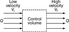
The rate of change of momentum for the control volume is the force on the control volume and is given by:
For the fire hose this would be the force on the nozzle, but normally we calculate in terms of the force on the liquid. This is equal in size but opposite in direction, so finally:
We shall now go on to consider three applications of liquid jets, but it is important to note that this equation is the only one to remember.
Normal impact on a flat plate
A jet of liquid is directed to hit a flat polished plate with a normal impact, i.e. perpendicular to the plate in all directions so that the picture is symmetrical, as shown in Figure 3.2.27.

If this is carried out with the nozzle and the plate fixed firmly, then the water runs exceptionally smoothly along the plate without any rebound. Therefore in the x-direction the final velocity of the jet is zero since the water ends up travelling radially along the plate. Due to the symmetry, the forces along the plate must cancel out and leave only the force in the x-direction.

The negative sign indicates that the force on the liquid is from right to left, so the force on the plate is from left to right:
In this case the direction is obvious but in later examples it will be less clear so it is best to learn the sign convention now.
Example 3.2.6
A jet of water emerges from a 20 mm diameter nozzle at a flow rate of 0.04 m3/s and impinges normally onto a flat plate. Calculate the force experienced by the plate.
The equation to use here is Equation (3.2.10), but first we need to calculate the mass flow rate and the initial velocity.
This is the initial velocity and the final velocity is zero in the direction of the jet. Hence:
The force on the plate is +5.09 kN, in the direction of the jet.
Impact on an inclined flat plate (Figure 3.2.28)
In this case the symmetry is lost and it looks as though we will have to resolve forces in the x- and y-directions. However, we can avoid this by using some commonsense and a little knowledge of fluid mechanics. In the y-direction there could only be a force on the plate if the liquid had a very large viscosity to produce an appreciable drag force. Most of the applications for this type of calculation are to do with water turbines and, as we have seen in earlier sections, water has a very low viscosity. Therefore we can neglect any forces in the y-direction, leaving only the x-direction.
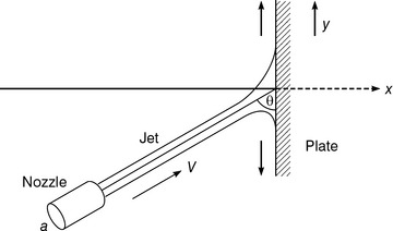
The final velocity in the x-direction is zero, as in the previous example, but the initial velocity is now v sin θbecause of the inclination of the jet to the x-axis. The velocity to be used in the part of the calculation which relates to the mass flow rate is still the full velocity; however, since the mass flow rate is the same whether the plate is there or not, let alone whether it is inclined.
Therefore the force on the plate is
Stationary curved vane
This is a simplified introduction to the subject of turbines and involves changes of momentum in the x- and y-directions. Since the viscosity is low and the vanes are always highly polished, we can assume initially that the liquid jet runs along the surface of the vane without being slowed down by any frictional drag (Figure 3.2.29).

Fx and Fy are calculated separately from the formula ![]()

These two components can then be combined using a rectangle of forces and Pythagoras’ theorem to give a single resultant force. The force on the turbine blade is equal and opposite to this resultant force on the liquid.
In practice the liquid does not leave the vane at quite the same speed as it entered because of friction. Even so the amount of slowing is still quite small, and we can take it into account by simply multiplying the final velocities by some correction factor. For example, if the liquid was slowed by 20% then we would use a correction factor of 0.8 on the final velocity.
Forces on pipe bends
Newton’s second law relates to the forces caused by changes in velocity. Velocity is a vector quantity and so it has direction as well as magnitude. This means that a force will be required to change the direction of a flowing liquid, just as it is required to change the speed of the liquid. Therefore if a liquid flows along a pipeline which has a bend in it then a considerable force can be generated on the pipe by the liquid even though the liquid may keep the same speed throughout. In practical terms this is important because the supports for the pipe must be designed to be strong enough to withstand this force.
The calculation for such a situation is similar to that for the curved vane above except that pipe bends are usually right angles and so the working is easier. The liquid is brought to rest in the original direction and accelerated from rest up to full speed in the final direction. Hence the two components of force are of the same size, as long as the pipe diameter is constant round the bend, and the resultant force on the bend will be outwards and at 45° to each of the two arms of the pipe.
Problems 3.2.1
(1) Look back in this textbook and find out the SI unit for viscosity.
(2) Using the correct SI units to substitute into the expression for Reynolds number, show that Re is dimensionless.
(3) What is the Reynolds number for flow of an oil of density 920 kg/m3 and viscosity 0.045 Pa s along a tube of radius 20 mm with a velocity of 2.4 m/s?
(4) Liquid of density 850 kg/m3 is flowing at a velocity of 3 m/s along a tube of diameter 50 mm. What is the approximate value of the liquid’s viscosity if it is known that the flow is in the transition region?
(5) For the same conditions as in Problem 4, what would the diameter need to be to produce a Reynolds number of 12 000?
(6) Imagine filling a kettle from a domestic tap. By making assumptions about diameter and flow rate, and looking up values for density and viscosity, calculate whether the flow is laminar or turbulent.
(7) The cross-sectional area of the nozzle on the end of a hosepipe is 1000 mm2 and a pump forces water through it at a velocity of 25 m/s. Find (a) the volume flow rate, (b) the mass flow rate.
(8) Oil of relative density 0.9 is flowing along a pipe of internal diameter 40 cm at a mass flow rate of 45 tonne/hour. Find the mean flow velocity.
(9) A pipe tapers from an external diameter of 82 mm to an external diameter of 32 mm. The pipe wall is 2 mm thick and the volume flow rate of liquid in the pipe is 45 litres/min. Find the flow velocity at each end of the pipe.
(10) In the pipe system in Figure 3.2.30 Find vA, vB, vC.
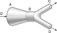
(11) Calculate the pressure differential which must be applied to a pipe of length 10.4 m and diameter 6.4 mm to make a liquid of viscosity 0.12 Pa s flow through it at a rate of 16 litres/hour (1000 litres = 1 m3).
(12) Calculate the flow rate which will be produced when a pressure differential of 6.8 MPa is applied across a 7.6 m long pipe, of diameter 5 mm, containing liquid of viscosity 1.8 Pa s.
(13) Referring to Figure 3.2.31, calculate the distance of the join in the pipes away from the right-hand end.
(14) Referring to Figure 3.2.32, calculate the flow rate from the outlet pipe.

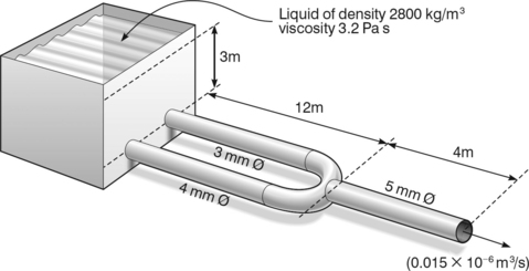
(15) Water is flowing along a pipe of diameter 0.2 m at a rate of 0.226 m3/s. What is the velocity head of the water, and what is the corresponding pressure?
(16) Water is flowing along a horizontal pipe of internal diameter 30 cm, at a rate of 60 m3/min. If the pressure in the pipe is 50 kN/m2 and the pipe centre is 6 m above ground level, find the total head of the water relative to the ground.
(17) Oil of relative density 0.9 flows along a horizontal pipe of internal diameter 40 cm at a rate of 50 m3/min. If the pressure in the pipe is 45 kPa and the centre of the pipe is 5 m above ground level, find the total head of the oil relative to the ground.
(18) The pipe in Problem 17 joins a smaller pipe of internal diameter 35 cm which is at a height of 0.3 m above the ground. What will be the pressure of the oil in this second pipe?
(19) In a horizontal Venturi meter the pipe diameter is 450 mm, the throat diameter is 150 mm, and the discharge coefficient is 0.97. Determine the volume flow rate of water in the meter if the difference in levels in a mercury differential U-tube manometer connected between the inlet pipe and the throat is 225 mm.
(20) A horizontal Venturi meter with a main diameter of 30 mm and a throat diameter of 16 mm is sited on a new lunar field station. It is being used to measure the flow rate of methylated spirits, of relative density 0.8. The difference in levels between simple manometer tubes connected to the inlet and the throat is 220 mm. Calculate the mass rate of flow.
(21) An orifice meter consists of a 100 mm diameter orifice in a 250 mm diameter pipe and has a discharge coefficient of 0.65. The pipe conveys oil of relative density 0.9 and the pressure difference between the sides of the orifice plate is measured by a mercury U-tube manometer which shows a reading of 760 mm. Calculate the volume flow rate in the pipeline.
(22) An orifice meter is installed in a vertical pipeline to measure the upwards flow of a liquid polymer, of relative density 0.9. The pipe diameter is 100 mm, the orifice diameter is 40 mm and the discharge coefficient is 0.6. The pressure difference across the orifice plate, measured from a point 100 mm upstream to a point 50 mm downstream, is 8.82 kPa.
Starting with Bernoulli’s equation and remembering to take into account the height difference between the pressure tappings, find the volume rate of flow along the pipe.
(23) A Pitot tube is pointed directly upstream in a fast flowing river, showing a reading of 0.459 m. Calculate the velocity of the river.
(24) For a liquid flowing along a pipe at 10.8 m/s calculate the height difference between levels in a Pitot-static tube.
(25) A powerboat is to be raced on the Dead Sea, where the relative density of the salt water is 1.026. The speed will be monitored by a Pitot-static tube mounted underneath and connected to a pressure gauge. Calculate the pressure differences corresponding to a speed of 70 km/hour.
(26) A prototype aeroplane is being tested and the only means of establishing its speed is a simple Pitot-static tube with both leads connected to a mercury U-tube manometer. Calculate the speed if the manometer reading is 356 mm.
(27) Water is flowing along a pipe at a rate of 24 m3/min from point A, area 0.3 m2, to point B, area 0.03 m2, which is 15 m lower. If the pressure at A is 180 kN/m2 and the loss of total head between A and B is 0.6 m, find the pressure at B.
(28) Water flows downwards through a pipe at a rate of 0.9 m3/min from point A, diameter 100 mm, to point B, diameter 50 mm, which is 1.5 m lower. PA = 70 kPa, PB = 50 kPa. Find the head loss between A and B.
(29) Water is flowing along a horizontal pipe of diameter 0.2 m, at a rate of 0.226 m3/s. The pipe has a 90° threaded elbow, a 90° mitred elbow and a fully open globe valve, all fitted into a short section. Find:
(30) A short piping system is as shown in Figure 3.2.33. Calculate the loss of total head caused by the pipe fittings and hence find the pressure at point B, using the table on p. 155.

(31) Calculate the head loss due to friction in a 750 m long pipe of diameter 620 mm when the flow rate is 920 m3/hour and the friction factor f = 0.025.
(32) A pressure drop of 760 kPa is caused when oil of relative density 0.87 flows along a pipe of length 0.54 km and diameter 0.18 m at a rate of 3000 m3/hour. Calculate the friction factor.
(33) A head loss of 5.6 m is produced when water flows along an 850 m long pipe of radius 0.12 m which has a friction factor of 0.009. Calculate the flow rate of the water in tonnes/hour.
(34) Liquid of relative density 1.18 flows at a rate of 3240 tonnes/hour along a 0.8 km long pipe, of diameter 720 mm and friction factor 0.00095. Calculate the gradient at which the pipe must fall in order to maintain a constant internal pressure.
(35) The volume rate of flow of a liquid in a 300 mm diameter pipe is 0.06 m3/s. The liquid has viscosity of 1.783 × 10⁻⁵ Pas and relative density 0.7. The equivalent surface roughness of the pipe is 0.6 mm.
(a) Determine Re and state whether the flow is turbulent.
(b) Determine f from a Moody chart.
(c) Determine the pressure drop over a 100 m horizontal length of pipe.
(36) Determine the head loss due to friction when water flows through 300 m of 150 mm dia galvanized steel pipe at 50 l/s.
(37) Determine the size of galvanized steel pipe needed to carry water a distance of 180 m at 85 l/s with a head loss of 9 m. (Conditions as above in Problem 36.)
This is an example of designing a pipe system where the Moody chart has to be used in reverse. Assume turbulent flow and be prepared to iterate. Finally you must calculate Re to show that your assumption of the turbulent flow was correct.
(38) A flat rectangular plate is suspended by a hinge along its top horizontal edge. The centre of gravity of the plate is 100 mm below the hinge. A horizontal jet of water of diameter 25 mm impinges normally on to the plate 150 mm below the hinge with a velocity of 5.65 m/s. Find the horizontal force which needs to be applied to the centre of gravity to keep the plate vertical.
(39) The velocity of the jet in Problem 38 is increased so that a force of 40 N is now needed to maintain the vertical position. Find the new value of the jet velocity.
(40) The nozzle of a fire hose produces a 50 mm diameter jet of water when the discharge rate is 0.085 m3/s. Calculate the force of the water on the nozzle if the jet velocity is 10 times the velocity of the water in the main part of the hose.
(41) A jet of water, of cross-section area 0.01 m2 and discharge rate 100 kg/s, is directed horizontally into a hemispherical cup so that its velocity is exactly reversed. If the cup is mounted at one end of a 4.5 m bar which is supported at the other end, find the torque produced about the support by the jet.
(42) A helicopter with a fully laden weight of 19.6 kN has a rotor of 12 m diameter. Find the mean vertical velocity of the air passing through the rotor disc when the helicopter is hovering. (Density of air = 1.28 kg/m3)
(43) A horizontal jet of water of diameter 25 mm and velocity 8 m/s strikes a rectangular plate of mass 5.45 kg which is hinged along its top horizontal edge. As a result the plate swings to an angle of 30° to the vertical. If the jet strikes at the centre of gravity, 100 mm along the plate from the hinge, find the horizontal force which must be applied 150 mm along the plate from the hinge to keep it at that angle.
(44) A 15 mm diameter nozzle is supplied with water at a total head of 30 m. 97% of this head is converted to velocity head to produce a jet which strikes tangentially a vane that is curved back on itself through 165°. Calculate the force on the vane in the direction of the jet (the x-direction) and in the y-direction.
(45) If the jet in Problem 44 is slowed down to 80% of its original value in flowing over the vane, calculate the new x and y forces.