5.4 Beams
A beam can be defined as a structural member which is subject to forces causing it to bend and is a very common structural member. This section is about such structural members and the analysis of the forces, moments and stresses concerned.
Bending occurs when forces are applied which have components at right angles to the member axis and some distance from a point of support; as a consequence beams become curved. Generally beams are horizontal and the loads acting on the beam act vertically downwards.
Beams
The following are common types of beams:
• Cantilever (Figure 5.4.1(a)) This is rigidly fixed at just one end, the rigid fixing preventing rotation of the beam when a load is applied to the cantilever. Thus there will be a moment due to a load and this, for equilibrium, has to be balanced by a resisting moment at the fixed end. At a free end there are no reactions and no resisting moments.

Figure 5.4.1 Examples of beams: (a) cantilever; (b) simply supported; (c) simply supported with overhanging ends; (d) built-in
• Simply supported beam (Figure 5.4.1(b)) This is a beam which is supported at its ends on rollers or smooth surfaces or one of these combined with a pin at the other end. At a supported end or point there are reactions but no resisting moments.
• Simply supported beam with overhanging ends (Figure 5.4.1(c)) This is a simple supported beam with the supports set in some distance from the ends. At a support there are reactions but no resisting moments; at a free end there are no reactions and no resisting moments.
• Built-in beam (encastre) (Figure 5.4.1(d)) This is a beam which is built-in at both ends and so both ends are rigidly fixed. Where an end is rigidly fixed there is a reaction force and a resisting moment.
The loads that can be carried by beams may be concentrated or distributed. A concentrated load is one which can be considered to be applied at a point while a distributed load is one that is applied over a significant length of the beam. With a distributed load acting over a length of beam, the distributed load may be replaced by an equivalent concentrated load at the centre of gravity of the distributed length. For a uniformly distributed load, the centre of gravity is at the midpoint of the length (Figure 5.4.2). Loading on a beam may be a combination of fixed loads and distributed loads.

Beams can have a range of different forms of section and the following (Figure 5.4.3) are some commonly encountered forms:

• Simple rectangular sections, e.g. as with the timber joists used in the floor construction of houses. Another example is the slab which is used for floors and roofs in buildings; this is just a rectangular section beam which is wide and shallow.
• An I-section, this being termed the universal beam. The universal beam is widely used and available from stockists in a range of sizes and weights. The I-section is an efficient form of section in that the material is concentrated in the flanges at the top and bottom of the beam where the highest stresses will be found.
• Circular sections or tubes, e.g. tubes carrying liquids and supported at a number of points.
Shear force and bending moment
There are two important terms used in describing the behaviour of beams: shear force and bending moment. Consider a cantilever (Figure 5.4.4(a)) which has a concentrated load F applied at the free end. If we make an imaginary cut through the beam at a distance x from the free end, we will think of the cut section of beam (Figure 5.4.4(b)) as a free body, isolated from the rest of the beam and effectively floating in space. With just the force indicated in Figure 5.4.4(b)), the body would not be in equilibrium. However, since it is in equilibrium, we must have for vertical equilibrium a vertical force V acting on it such that V = F (Figure 5.4.4(c)). This force V is called the shear force because the combined action of V and F on the section is to shear it (Figure 5.4.5). In general, the shear force at a transverse section of a beam is the algebraic sum of the external forces acting at right angles to the axis of the beam on one side of the section concerned.


In addition to vertical equilibrium we must also have the section of beam in rotational equilibrium. For this we must have a moment M applied (Figure 5.4.4(d)) at the cut so that M = Fx. This moment is termed the bending moment. In general, the bending moment at a transverse section of a beam is the algebraic sum of the moments about the section of all the forces acting on one (either) side of the section concerned.
Sign conventions
The conventions most often used for the signs of shear forces and bending moments are:
When the left-hand side of the beam section is being pushed upwards and the right-hand side downwards, i.e. the shear forces on either side of the section are in a clockwise direction, then the shear force is taken as being positive (Figure 5.4.6(a)). When the left-hand side of the beam is being pushed downwards and the right-hand side upwards, i.e. when the shear forces on either side of a section are in an anticlockwise direction, the shear force is taken as being negative (Figure 5.4.6(b)).

Bending moments are positive if they give rise to sagging (Figure 5.4.7(a)) and negative if they give rise to hogging (Figure 5.4.7(b)).

Example 5.4.1
Determine the shear force and bending moment at points 0.5 m and 1.5 m from the left-hand end of a beam of length 4.5 m which is supported at its ends and subject to a point load of 9 kN a distance of 1.5 m from the left-hand end (Figure 5.4.8). Neglect the weight of the beam.

Figure 5.4.8 Example 5.4.1
The reactions at the supports can be found by taking moments about the left-hand end support A:
to give RB = 3 kN. Since, for vertical equilibrium we have:
then RA = 6 kN. The forces acting on the beam are thus as shown in Figure 5.4.9.

Figure 5.4.9 Example 5.4.1
If we make an imaginary cut in the beam at 3.5 m from the left-hand end (Figure 5.4.9), then the force on the beam to the right of the cut is 3 kN upwards and that to the left is 9 − 6 = 3 kN downwards. The shear force V is thus negative and −3 kN.
If we make an imaginary cut in the beam at 0.5 m from the left-hand end (Figure 5.4.10), then the force on the beam to the right of the cut is 9 − 3 = 6 kN downwards and that to the left is 6 kN upwards. The shear force V is thus positive and +6 kN.

Figure 5.4.10 Example 5.4.1
The bending moment at a distance of 3.5 m from the left-hand end of the beam, for that part of the beam to the right, is 3 × 1 = 3 kNm. Since the beam is sagging the bending moment is +3 kNm. At a distance of 0.5 m from the left-hand end of the beam, the bending moment, for that part of the beam to the right, is 3 × 4 − 9 × 0.5 = +7.5 kN m.
Example 5.4.2
A uniform cantilever of length 3.0 m (Figure 5.4.11) has a uniform weight per metre of 120 kN. Determine the shear force and bending moment at distances of (a) 1.0 m and (b) 3.0 m from the free end if no other loads are carried by the beam.

Figure 5.4.11 Example 5.4.2
(a) With a cut 1.0 m from the free end, there is 1.0 m of beam to the right with a weight of 120 kN (Figure 5.4.12(a)). Thus, since the total force on the section to the right of the cut is 120 kN the shear force V is +120 kN; it is positive because the forces are clockwise.

Figure 5.4.12 Example 5.4.2
The weight of this section can be considered to act at its centre of gravity which, because the beam is uniform, is at its midpoint. Thus the 120 kN weight force can be considered to be 0.5 m from the cut end of the right-hand section and so the bending moment is −120 × 0.5 = −60 kN m; it is negative because there is hogging.
(b) At 3.0 m from the free end, there is 3.0 m of beam to the right and it has a weight of 360 kN (Figure 5.4.12(b)). Thus, since the total force on the section to the right of the cut is 360 N the shear force V is +360 kN; it is positive because the forces are clockwise.
The weight of this section can be considered to act at its midpoint, a distance of 1.5 m from the free end. Thus the bending moment is −360 × 1.5 = −540 kN m; it is negative because there is hogging.
Shear force and bending moment diagrams
Shear force diagrams and bending moment diagrams are graphs used to show the variations of the shear forces and bending moments along the length of a beam. The convention that is generally adopted is to show positive shear forces and bending moments plotted above the axial line of the beam and below it if negative.
Simply supported beam with point load at mid-span
For a simply supported beam with a central load F (Figure 5.4.13), the reactions at each end will be F/2.

Figure 5.4.13 (a) Simply supported beam with point load; (b) shear force diagram; (c) bending moment diagram
At point A, the forces to the right are F − F/2 and so the shear force at A is +F/2. This shear force value will not change as we move along the beam from A until point C is reached. To the right of C we have just a force of −F/2 and this gives a shear force of − F/2. To the left of C we have just a force of +F/2 and this gives a shear force of +F/2. Thus at point C, the shear force takes on two values. Figure 5.4.13(b) shows the shear force diagram.
At point A, the moments to the right are F × L/2 − F/2 × L = 0. The bending moment is thus 0. At point C the moment to the right is F/2 × L/2 and so the bending moment is + FL/4; it is positive because sagging is occurring. At point B the moment to the left is F × L/2 − F/2 × L = 0. Between A and C the bending moment will vary, e.g. at one-quarter the way along the beam it is FL/8. In general, between A and C the bending moment a distance x from A is Fx/2 and between C and B is Fx/2 − F (x −L/2) = F/2(L − x). Figure 5.4.13(c) shows the bending moment diagram. The maximum bending moment occurs under the load and is ![]() FL.
FL.
Simply supported beam with uniformly distributed load
A simply supported beam which carries just a uniformly distributed load of w/unit length (Figure 5.4.14) will have the reactions at each end as wL/2.

Figure 5.4.14 (a) Simply supported beam with distributed load; (b) shear force diagram; (c) bending moment diagram
For the shear force a distance x from the left-hand end of the beam, the load acting on the left-hand section of beam is wx and thus the shear force is:
When ![]() , the shear force is zero. When
, the shear force is zero. When ![]() the shear force is positive and when
the shear force is positive and when ![]() it is negative. Figure 5.4.14(b) shows the shear force diagram.
it is negative. Figure 5.4.14(b) shows the shear force diagram.
At A the moment due to the beam to the right is −wL × L/2 + wL/2 × L = 0. At the midpoint of the beam the moment is − wL/2 × L/4 + wL/2 × L/2 = wL2/8 and so the bending moment is +wL2/8. At the quarter-point along the beam, the moment due to the beam to the right is −3L/4 × 3L/8 + wL/2 × 3L/4 = 3wL2/32. In general, the bending moment due to the beam at distance x from A is:
Differentiating the equation gives dM/dx = − wx + wL/2. Thus dM/dx = 0 at x = L/2. The bending moment is thus a maximum at x = L/2 and so the bending moment at this point is wL2/8. Figure 5.4.14(c) shows the bending moment diagram.
Cantilever with point load at free end
For a cantilever which carries a point load F at its free end (Figure 5.4.15(a)) and for which the weight of the beam is neglected, the shear force at any section will be +F, the shear force diagram thus being as shown in Figure 5.4.15(b). The bending moment at a distance x from the fixed end is:
The minus sign is because the beam shows hogging. We have dM/dx =F and thus the bending moment diagram is a line of constant slope F. At the fixed end, when x = 0, the bending moment is FL. At the free end, when x = L, the bending moment is 0.

Cantilever with uniformly distributed load
Consider a cantilever which has just a uniformly distributed load of w per unit length (Figure 5.4.16(a)). The shear force a distance x from the fixed end is:
Thus at the fixed end the shear force is +wL and at the free end it is 0. Figure 5.4.16(b) shows the shear force diagram. The bending moment at a distance x from the fixed end is, for the beam to the right of the point, given by:
This is a parabolic function. At the fixed end, where x = 0, the bending moment is ![]() . At the free end the bending moment is 0. Figure 5.4.16(c) shows the bending moment diagram.
. At the free end the bending moment is 0. Figure 5.4.16(c) shows the bending moment diagram.

General points about shear force and bending moment diagrams
From the above examples of beams, we can conclude that:
• Between point loads, the shear force is constant and the bending moment variation with distance is a straight line.
• Throughout a length of beam which has a uniformly distributed load, the shear force varies linearly with distance and the bending moment varies with distance as a parabola.
• The bending moment is a maximum when the shear force is zero.
• The shear force is a maximum when the slope of the bending moment diagram is a maximum and zero when the slope is zero.
• For point loads, the shear force changes abruptly at the point of application of the load by an amount equal to the size of the load.
Maximum value of the bending moment occurs at a point of zero shear force
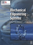
The following is a proof of the above statement. Consider a very small segment of beam (Figure 5.4.17) of length δx and which is supporting a uniformly distributed load of w per unit length. The load on the segment is w δ x and can be considered to act through its centre. The values of the shear force V and bending moment M increase by δV and δM from one end of the segment to the other.
If we take moments about the left-hand edge of the segment then:
Neglecting multiples of small quantities gives V δ x = δM and hence, as δx tends to infinitesimally small values, we can write:
Thus, the shear force is the gradient of the bending moment –distance graph and so V = 0 when this gradient dM/dx = 0. The gradient of a curve is zero when it is a maximum or a minimum. Thus a local maximum or minimum bending moment occurs when the shear force is zero.
Integrating the above equation gives:
Hence the bending moment at any point is represented by the area under the shear force diagram up to that point.
Example 5.4.3
A cantilever has a length of 3 m and carries a point load of 3 kN at a distance of 2 m from the fixed end and a uniformly distributed load of 2 kN/m over a 2 m length from the fixed end. Draw the shear force and bending moment diagrams and determine the position and size of the maximum bending moment and maximum shear force.
Figure 5.4.18(a) shows the beam. To the right of C there are no forces and so the shear force for that section of the beam is zero. To the right of A the total force is 4 + 3 = 7 kN and so this is the value of the shear force at A. At a point 1 m from A the total force to the right is 2 + 3 = 5 kN and so this is the shear force at that point. The shear force a distance x from A, with x less than 2 m, is 2(2 − x) + 3 kN. At C, when x = 2, the shear force is 3 kN. Figure 5.4.18(b) shows the shear force diagram.

Figure 5.4.18 Example 5.4.3
The bending moment at C for the beam to the right is 0. At A the bending moment for the beam to the right is –(4 × 1 + 2 × 3) = −10 kN m; it is negative because there is hogging. At a distance x from the fixed end, the bending moment is −[2(2 − x) ×![]() (2 − x) + 3 ×(2 − x)] kN m. Figure 5.4.18(c) shows the resulting bending moment diagram.
(2 − x) + 3 ×(2 − x)] kN m. Figure 5.4.18(c) shows the resulting bending moment diagram.
The maximum bending moment will be at a point on the shear force diagram where the shear force is zero and is thus at the fixed end and has the value 10 kN m.
Example 5.4.4
A beam of length 4 m is supported at its ends and carries loads of 80 N and 120 N at 1 m and 2 m from one end (Figure 5.4.19(a)). Draw the shear force and bending moment diagrams and determine the position and size of the maximum bending moment. Neglect the weight of the beam.

Figure 5.4.19 Example 5.4.4
Hence R2 = 80 N. Since R1 + R2 = 80 + 120, then R1 = 120 N.
At any point in AC the shear force is 80 + 120 − 80 = 120 N. In CD the shear force is 120 − 80 = 40 N. In DB the shear force is −80 N. Figure 5.4.19(b) shows the resulting shear force diagram.
At any point a distance x from A in AC the bending moment is 120x, reaching 120 Nm at C. At any point a distance x from A in CD the bending moment is 120x − 80(x − 1) = 40x + 80, reaching 160 Nm at D. At any point a distance x from A in DB the bending moment is 120x − 80(x − 1) −120(x − 2) = −80x + 320, reaching 0 at B. Figure 5.4.19(c) shows the resulting bending moment diagram.
Localized maximum bending moments will be at points on the shear force diagram where the shear force is zero. The maximum is at 2 m from A and has the value 160 Nm.
Bending stress
The following is a derivation of equations which enable us to determine the stresses produced in beams by bending. When a bending moment is applied to a beam it bends, as in Figure 5.4.20, and the upper surface becomes extended and in tension and the lower surface becomes compressed and in compression. The upper surface increasing in length and the lower surface decreasing in length implies that between the upper and lower surface there is a plane which is unchanged in length when the beam is bent. This plane is called the neutral plane and the line where the plane cuts the cross-section of the beam is called the neutral axis.

Figure 5.4.20 Bending stretches the upper surface and contracts the lower surface, in between there is an unchanged in length surface
Consider a beam, or part of a beam, and assume that it is bent into a circular arc. A section through the beam aa which is a distance y from the neutral axis (Figure 5.4.21) has increased in length as a consequence of the beam being bent and the strain it experiences is the change in length ΔL divided by its initial unstrained length L. For circular arcs, the arc length is the radius of the arc multiplied by the angle it subtends, and thus, L + ΔL = (R + y)θ. The neutral axis NA will, by definition, be unstrained and so for it we have L = Rθ. Hence, the strain on aa is:

The strain thus varies linearly through the thickness of the beam being larger the greater the distance y from the neutral axis. The maximum strains thus occur at the outer surfaces of a beam, these being the most distant from the neutral axis.
Provided we can use Hooke’s law, the stress due to bending which is acting on aa is:
The maximum stresses thus occur at the outer surfaces of a beam, these being the most distant from the neutral axis. Figure 5.4.22 shows how the stress will vary across the section of rectangular cross-section beam, such a beam having a central neutral axis. It is because the highest stresses will be at the maximum distances from the neutral axis that the I-section girder makes most effective use of material, placing most material where the stresses are the highest.

The general bending equations
For the beam, shown in Figure 5.4.21, which has been bent into the arc of a circle, if the element aa has a cross-sectional area δA in the cross-section of the beam at a distance y from the neutral axis of radius R, the element will be stretched as a result of the bending with stress σ= Ey/R, where E is the modulus of elasticity of the material. The forces stretching this element aa are:
The moment of the force acting on this element about the neutral axis is:
The total moment M produced over the entire cross-section is the sum of all the moments produced by all the elements of area in the cross-section. Thus, if we consider each such element of area to be infinitesimally small, we can write:
The integral is termed the second moment of area I of the section:
Thus we can write:
Since the stress σon a layer a distance y from the neutral axis is yE/R:
The above two equations are generally combined and written as the general bending formula:
This formula is only an exact solution for the case of pure bending, i.e. where the beam is bent into the arc of a circle. This only occurs where the bending moment is constant; however, many beam problems involve bending moments which vary along the beam. The equation is generally still used since it provides answers which are usually accurate enough for engineering design purposes.
Example 5.4.5
A uniform rectangular cross-section horizontal beam of length 4 m and depth 150 mm rests on supports at its ends (Figure 5.4.23) and supports a concentrated load of 10 kN at its midpoint. Determine the maximum tensile and compressive stresses in the beam if it has a second moment of area of 2.8 × 10⁻⁵ m4 and the weight of the beam can be neglected.

Figure 5.4.23 Example 5.4.5
Taking moments about the left-hand end gives 4R2 = 2 × 10 and so R2 = 5 kN. Since R1 + R2 = 10 then R1 = 5 kN. The maximum bending moment will occur at the midpoint and is 10 kN m. The maximum bending stress will occur at the cross-section where the bending moment is a maximum and on the outer surfaces of the beam, i.e. y = ±75 mm. Hence:
Section modulus
For a beam which has been bent, the maximum stress σmax will occur at the maximum distance ymax from the neutral axis. Thus:
The quantity I/ymax is a purely geometric function and is termed the section modulus Z. Thus we can write:
with:
Figure 5.4.24 gives values for typical sections. Standard section handbooks give values of the second moment of area and section modulus for different standard section beams, Table 5.4.1 being an illustration of the information provided.


Figure 5.4.25 Table 5.4.1
Example 5.4.6
A beam has a section modulus of 3 × 106mm3, what is the maximum bending moment that can be used if the stress in the beam must not exceed 6 MPa?
Example 5.4.7
A rectangular cross-section beam of length 4 m rests on supports at each end and carries a uniformly distributed load of 10 kN/m. If the stress must not exceed 8 MPa, what will be a suitable depth for the beam if its width is 100 mm?
For a simply supported beam with a uniform distributed load over its full length, the maximum bending moment is wL2/8 and thus the maximum bending moment for this beam is 10 × 42/8 = 20 kNm. Hence, the required section modulus is:
For a rectangular cross-section Z = bd2/6 and thus:
A suitable beam might thus be one with a depth of 400 mm.
Moments of area
The product of an area and its distance from some axis is called the first moment of area; the product of an area and the square of its distance from an axis is the second moment of area. By considering the first moment of area we can determine the location of the neutral axis; the second moment of area enables us, as indicated above, to determine the stresses present in bent beams.
First moment of area and the neutral axis
In the above discussion of the bending of beams it was stated that the position of the neutral axis for a rectangular cross-section beam was its central axis. Here we derive the relationship which enables the position of the neutral axis to be determined for any cross-section. Consider a beam bent into the arc of a circle. The forces acting on a segment a distance y from the neutral axis are:
The total longitudinal force will be the sum of all the forces acting on such segments and thus, when we consider infinitesimally small areas, is given by:
But since the beam is only bent, it is only acted on by a bending moment and there is no longitudinal force stretching the beam. Thus, since E and R are not zero, we must have:
The integral ![]() y dA is called the first moment of area of the section.
y dA is called the first moment of area of the section.
The only axis about which we can take such a moment and obtain 0 is an axis through the centre of the area of the cross-section, i.e. the centroid of the beam. Thus the neutral axis must pass through the centroid of the section when the beam is subject to just bending. Hence we can determine the position of the neutral axis by finding the position of the centroid.
Example 5.4.8
Determine the position of the neutral axis for the T-section beam shown in Figure 5.4.26

Figure 5.4.26 Example 5.4.8
The neutral axis will pass through the centroid. We can consider the T-section to be composed of two rectangular sections with the centroid of each at its centre. Hence, taking moments about the base of the T-section:
Hence the distance of the centroid from the base is (total moment)/(total area):
Second moment of area
The integral ![]() y2 dA defines the second moment of area I about an axis and can be obtained by considering a segment of area δA some distance y from the neutral axis, writing down an expression for its second moment of area and then summing all such strips that make up the section concerned, i.e. integrating. As indicated in the discussion of the general bending equation, the second moment of area is needed if we are to relate the stress produced in a beam to the applied bending moment.
y2 dA defines the second moment of area I about an axis and can be obtained by considering a segment of area δA some distance y from the neutral axis, writing down an expression for its second moment of area and then summing all such strips that make up the section concerned, i.e. integrating. As indicated in the discussion of the general bending equation, the second moment of area is needed if we are to relate the stress produced in a beam to the applied bending moment.
As an illustration of the derivation of a second moment of area from first principles, consider a rectangular cross-section of breadth b and depth d (Figure 5.4.27). For a layer of thickness δy a distance y from the neutral axis, which passes through the centroid, the second moment of area for the layer is:

Example 5.4.9
Determine the second moment of area about the neutral axis of the I-section shown in Figure 5.4.28.

Figure 5.4.28 Example 5.4.9
We can determine the second moment of area for such a section by determining the second moment of area for the entire rectangle containing the section and then subtracting the second moments of area for the rectangular pieces ‘missing’ (Figure 5.4.29).

Figure 5.4.29 Example 5.4.9
Thus for the rectangle containing the entire section, the second moment of area is given by I = bd3/12 = (50 × 703)/12 = 1.43 × 106mm4. Each of the ‘missing’ rectangles will have a second moment of area of (20 × 503)/12 = 0.21 × 106 mm4. Thus the second moment of area of the I-section is 1.43 × 10⁶ − 2 × 0.21 × 106 = 1.01 × 106mm4.
Parallel axis theorem
The parallel axis theorem is useful when we want to determine the second moment of area about an axis which is parallel to the one for which we already know the second moment of area. If we had a second moment of area I = ![]() y2 dA of an area about an axis and then considered a situation where the area was moved by a distance h from the axis, the new second moment of area Ih, would be:
y2 dA of an area about an axis and then considered a situation where the area was moved by a distance h from the axis, the new second moment of area Ih, would be:
But ![]() and
and ![]() . Hence:
. Hence:

Thus the second moment of area of a section about an axis parallel with an axis through the centroid is equal to the second moment of area about the axis through the centroid plus the area of the section multiplied by the square of the distance between the parallel axes. This is called the theorem of parallel axes.
Example 5.4.10
Determine, using the theorem of parallel axes, the second moment of area about the neutral axis of the I-section shown in Figure 5.4.28.
This is a repeat of Example 5.4.9. Consider the section as three rectangular sections with the web being the central rectangular section and the flanges a pair of rectangular sections with their neutral axes displaced from the neutral axis of the I-section by 30 mm (Figure 5.4.30). The central rectangular section has a second moment of area of I = bd3/12 = (10 × 503)/12 = 0.104 × 106mm4. Each of the outer rectangular areas will have a second moment of area given by the theorem of parallel axes as Ih = I + Ah2 = (50 × 103)/12 + 50 × 10 × 302 = 0.454 × 106 mm4. Thus the second moment of area of the I-section is 1.01 × 106mm4.

Figure 5.4.30 Example 5.4.10
Perpendicular axis theorem
The perpendicular axis theorem is useful when we want the second moment of area about an axis which is perpendicular to one about which we already know the second moment of area. Consider the second moment of an area with respect to an axis which is perpendicular to the plane of a section. Such an axis is termed the polar axis. Thus for the elemental section δA shown in Figure 5.4.31, this is the z-axis. The second moment of area of this section about the x-axis is:
The second moment of area of this section about the y-axis is:
Thus:
But r2 = y2 + x2 and thus
Since r is the distance of the elemental area from the z-axis, then the integral of r2 dA is the second moment of area Iz about that axis, often termed the polar second moment. Thus:
Thus the second moment of area with respect to an axis through a point perpendicular to a section is equal to the sum of the second moments of area with respect to any two mutually perpendicular axes in the plane of the area through the same point. This is known as the perpendicular axis theorem.

Second moments of area of a circular section
To obtain the second moment of area Iz about an axis perpendicular to the plane of the circular section, consider an annular element of radius r and thickness δr (Figure 5.4.32). The area of the element is 2πr dr. Thus:
This is the polar second moment of area. To obtain the second moments of area about two mutually perpendicular axes x and y we can use the perpendicular axes theorem. Since, as a result of symmetry, we have Ix = Iy, then:

Radius of gyration
A geometric property which is widely quoted for beams, of various cross-sections, is the radius of gyration k of a section. This is the distance from the axis at which the area may be imagined to be concentrated to give the same second moment of area I. Thus I = Ak2 and so:
Beam deflections
By how much does a beam deflect when it is bent as a result of the application of a bending moment? The following is a derivation of the basic differential equation which can be used to derive deflections. We then look at how we can solve the differential equation to obtain the required deflections.
The differential equation
When a beam is bent (Figure 5.4.33) as a result of the application of a bending moment M it curves with a radius R given by the general bending equation in 4.3.3 as:
This radius can be expressed in terms of the vertical deflection y as 1/R = d2y/dx2, where x is the distance along the beam from the chosen origin at which the deflection is measured, and so:
This differential equation provides the means by which the deflections of beams can be determined. The product EI is often termed the flexural rigidity of a beam.

The sign convention that is generally used is that deflections are measured in a downward direction and defined as positive and thus the bending moment is negative, since there is hogging. Hence, with this convention, the above equation is written as:
Figure 5.4.34 lists solutions of the above equation for some common beam loading situations.

This is a derivation of the differential equation describing the curvature of a beam when bent. Consider a beam which is bent into a circular arc and the radius R of the arc. For a segment of circular arc (Figure 5. 4.35), the angle δθ subtended at the centre is related to the arc length δs by δs = R δθ. Because the deflections obtained with beams are small δx is a reasonable approximation to δs and so we can write δx = R δθ and 1/R = δθ/δ x The slope of the straight line joining the two end points of the arc is and thus tan δθ = δy/δ x Since the angle will be small we can make the approximation that δθ = δy/δ x Hence:

Deflections by double integration
The deflection y of a beam can be obtained by integrating the differential equation d2y/dx2 = −M/EI with respect to x to give:
with A being the constant of integration and then carrying out a further integration with respect to x to give:
with B being a constant of integration.
At the point where maximum deflection occurs, the slope of the deflection curve will be zero and thus the point of maximum deflection can be determined by equating dy/dx to zero.
Example 5.4.12
Show that the deflection y at the free end of a cantilever (Figure 5.4.36) of length L when subject to just a point load F located at the free end is given by y = FL3/3EI.

Figure 5.4.36 Example 5.4.12
The bending moment a distance x from the fixed end is M = −F (L − x) and so the differential equation becomes:
Integrating with respect to x gives:
Since we have the slope dy/dx = 0 at the fixed end where x = 0, then we must have A = 0 and so:
Integrating again gives:
Since we have the deflection y = 0 at x = 0, then we must have B = 0 and so:
When x = L:
Example 5.4.13
Show that the deflection y at the mid-span of a beam of length L supported at its ends (Figure 5.4.37) and subject to just a uniformly distributed load of w/unit length is given by y = 5wL4/384EI.

Figure 5.4.37 Example 5.4.13
The bending moment a distance x from the left-hand end is M = ![]() wLx − wx
wLx − wx![]() x and so the differential equation becomes:
x and so the differential equation becomes:
Integrating with respect to x gives:
Since the slope dy/dx = 0 at mid-span where x = ![]() L, then A = wL3/24 and so:
L, then A = wL3/24 and so:
Integrating with respect to x gives:
Since y = 0 at x = 0, then B = 0 and so:
When x = ![]() L:
L:
Superposition
When a beam is subject to more than one load, while it is possible to write an equation for the bending moment and solve the differential equation, a simpler method is to consider the deflection curve and the deflection for each load separately and then take the algebraic sum of the separate deflection curves and deflections to give the result when all the loads are acting. The following example illustrates this.
Example 5.4.14
Determine the deflection curve for a cantilever of length L which is loaded by a uniformly distributed load of w/unit length over its entire length and a concentrated load of F at the free end.
For just a uniformly distributed load:
For just the concentrated load:
Thus the deflection curve when both loads are present is:
Macaulay’s method
For beams with a number of concentrated loads, i.e. where there are discontinuities in the bending moment diagram, we cannot write a single bending moment equation to cover the entire beam but have to write separate equations for each part of the beam between adjacent loads. Integration of each such expression then gives the slope and deflection relationships for each part of the beam. An alternative is to write a single equation using Macaulay’s brackets. The procedure is:
(1) Take the point from which distances are measured as the left-hand end of the beam. Denote the distance to a section as x.
(2) Write the bending moment expression at a section at the right-hand end of the beam in terms of the loads to the left of the section.
(3) Do not simplify the bending moment expression by expanding any of the terms involving the distance x which are contained within brackets. Indeed it is customary to use { } for such brackets since we will treat them differently from other forms of bracket.
(4) Integrate the bending moment equation, keeping all the bracketed terms within the { } brackets.
(5) Apply the resulting slope and deflection equations to any part of the beam but all terms within brackets which are negative are taken as being zero.
Where a distributed load does not extend to the right-hand end of the beam, as, for example, shown in Figure 5.4.38(a), then introduce two equal but opposite dummy loads, as in Figure 5.4.38(b). These two loads will have no net effect on the behaviour of the beam.

The following examples illustrate the use of this method to determine the deflections of beams.
Example 5.4.15
A beam of length 10 m is supported at its ends and carries a point load of 2 kN a distance of 4 m from the left-hand end and another point load of 5 kN a distance of 6 m from the left-hand end (Figure 5.4.39). Determine (a) the deflection under the 2 kN load, (b) the deflection under the 5 kN load and (c) the maximum deflection. The beam has a modulus of elasticity of 200 GPa and a second moment of area about the neutral axis of 108mm4.

Figure 5.4.39 Example 5.4.15
Taking moments about the left-hand end gives 10R2 = 4 × 2 + 6 × 5 and hence R2 = 3.8 kN. Since R1 + R2 = 7 then R1 = 3.2 kN.
For a section near the right-hand end a distance x from the left-hand end, the bending moment for the section to the left 3.2x − 2{x − 4} − 5{x − 6}. Hence:
Integrating with respect to x gives:
Integrating again with respect to x gives:
When x = 0, y = 0 and so B = 0. When x = 10, y = 0 and thus 0 = 0.53 × 1000 − 0.33 × 63 − 0.83 × 43 + 10 A and so A = −40.6.
(a) The deflection under the 2 kN load is at x = 4 m and thus we have:
Hence y = 128.5 × 10³/(200 × 109 × 108 × 10−12) = 8.5 × 10⁻³ m = 8.5 mm.
(b) The deflection under the 5 kN load is at x = 6 m and thus we have:
Hence y = 131.8 × 10³/(200 × 109 × 108 × 10−12) = 6.6 × 10⁻³ m = 6.6 mm.
(c) The maximum deflection occurs when dy/dx = 0 and so:
The maximum deflection can be judged to be between the two loads and thus we omit the {x − 6} term to give:

Using the equation for roots of a quadratic equation gives:
Hence the maximum deflection is given by:
Note that in the above equation the forces have been in kN. Hence y = 137.2 × 10³/(200 × 109 × 108 × 10−12) = 6.9 × 10⁻³m = 6.9 mm.
Example 5.4.16
A beam of length 8 m is supported at both ends and subject to a distributed load of 20 kN/m over the 4 m length of the beam from the left-hand support and a point load of 120 kN at 6 m from the left-hand support (Figure 5.4.40). Determine the mid-span deflection. The beam has a modulus of elasticity of 200 GPa and a second moment of area about the neutral axis of 108 mm4.

Figure 5.4.40 Example 5.4.16
Taking moments about the left-hand end gives, for the right-hand end support reaction R2, 8R2 = 80 × 2 + 120 × 6 and so R2 = 110 kN. Since R + R2 = 80 + 120, then R1 = 90 kN.
To apply the Macaulay method we need to introduce two dummy distributed loads so that distributed loads are continuous from the right-hand end. Thus the loads are as in Figure 5.4.41. The bending moment a distance x from the left-hand end is 90x −![]() x × 20x +
x × 20x + ![]() {x − 4} × 20{x − 4} − 120{x − 6}. Hence we can write:
{x − 4} × 20{x − 4} − 120{x − 6}. Hence we can write:
Integrating with respect to x gives:
Integrating again with respect to x gives:
When x = 0 we have y = 0 and so B = 0. When x = 8 then y = 0 and so the above equation gives 0 = −(15 × 83 − 10 × 84/12 + 10× 44/12 + 8A). Hence A = −540 and so we have:
The deflection at mid-span, i.e. x = 4, is thus:
Note that in the above equation the forces have been in kN. With El = 200 × 109 × 108 × 10−12 then y = 1413.3 × 103/(200 × 105) = 0.071 m.

Figure 5.4.41 Example 5.4.16
Problems 5.4.1
(1) A beam of length 4.0 m rests on supports at each end and a concentrated load of 100 N is applied at its midpoint. Determine the shear force and bending moment at distances of (a) 3.0 m, (b) 1.5 m from the left-hand end of the beam. Neglect the weight of the beam.
(2) A cantilever has a length of 2 m and a concentrated load of 1 kN is applied to its free end. Determine the shear force and bending moment at distances of (a) 1.5 m, (b) 1.0 m from the free end. Neglect the weight of the beam.
(3) A cantilever of length 4.0 m has a uniform weight per metre of 1 kN. Determine the shear force and bending moment at (a) 2.0 m, (b) 1.0 m from the free end. Neglect the weight of the beam.
(4) Draw the shear force and bending moment diagrams and determine the position and size of the maximum bending moment for the beams shown in Figure 5.4.42.
(5) Draw the shear force and bending moment diagrams for the beam shown in Figure 5.4.43.

(6) For a beam AB of length a + b which is supported at each end and carries a point load F at C, a distance a from A, show that (a) the shear force a distance x from A between A and C is Fb/(a + b) and the bending moment Fbx/(a + b), (b) between C and B the shear force is −Fa/(a + b) and the bending moment Fa(a + b − x)/(a + b), (c) the maximum bending moment is Fab/(a + b).
(7) A beam AB has a length of 9 m and is supported at each end. If it carries a uniformly distributed load of 6 kN/m over the 6 m length starting from A, by sketching the shear force and bending moment diagrams determine the maximum bending moment and its position.
(8) A beam AB has a length of 4 m and is supported at 0.5 m from A and 1.0 m from B. If the beam carries a uniformly distributed load of 6 kN/m over its entire length, by sketching the shear force and bending moment diagrams determine the maximum bending moment and its position.
(9) A beam AB has a length of 8 m and is supported at end A and a distance of 6 m from A. The beam carries a uniformly distributed load of 10 kN/m over its entire length and a point load of 80 kN a distance of 3 m from A and another point load of 65 kN a distance of 8 m from A. By sketching the shear force and bending moment diagrams determine the maximum bending moment and its position.
(10) By sketching the shear force and bending moment diagrams, determine the maximum bending moment and its position for the beam in Figure 5.4.44 where there is a nonuniform distributed load, the load rising from 0 kN/m at one end to 6 kN/m at the other end.

(11) A uniform rectangular cross-section horizontal beam of length 6 m and depth 400 mm rests on supports at its ends and supports a uniformly distributed load of 20 kN/m. Determine the maximum tensile and compressive stresses in the beam if it has a second moment of area of 140 × 106 mm4.
(12) A steel tube has a section modulus of 5 × 10⁻⁶ m3. What will be the maximum allowable bending moment on the tube if the bending stresses must not exceed 120 MPa?
(13) An I-section beam has a section modulus of 3990 cm3. What will be the maximum allowable bending moment on the beam if the bending stresses must not exceed 120 MPa?
(14) Determine the section modulus required of a steel beam which is to span a gap of 6 m between two supports and support a uniformly distributed load over its entire length, the total distributed load being 65 kN. The maximum bending stress permissible is 165 MPa.
(15) An I-section girder has a length of 6 m, a depth of 250 mm and a weight of 30 kN/m. If it has a second moment of area of 120 × 10−6 m4 and is supported at both ends, what will be the maximum stress?
(16) A rectangular section beam has a length of 4 m and carries a uniformly distributed load of 10 kN/m. If the beam is to have a width of 120 mm, what will be the maximum permissible beam depth if the maximum stress in the beam is to be 80 MPa?
(17) Determine the second moment of area of an I-section, about its horizontal neutral axis when the web is vertical, if it has rectangular flanges each 144 mm by 18 mm, a web of thickness 12 mm and an overall depth of 240 mm.
(18) Determine the second moment of area of a rectangular section 100 mm × 150 mm about an axis parallel to the 100 mm side if the section has a central hole of diameter 50 mm.
(19) A compound girder is made up of an I-section with a plate on the top flange, as shown in Figure 5.4.45. Determine the position of the neutral axis above the base of the section.

(20) Determine the position of the neutral axis above the base of the I-section shown in Figure 5.4.46.

(21) Determine the second moment of areas about the xx and yy axes through the centroid for Figure 5.4.47.

(22) Determine the radius of gyration of a section which has a second moment of area of 2.5 × 106mm4 and an area of 100 mm2.
(23) Determine the radius of gyration about an axis passing through the centroid for a circular area of diameter d and in the plane of that area.
(24) Determine the position of the neutral axis xx and the second moment of area Ixx about the neutral axis for the sections shown in Figure 5.4.48.

(25) Determine the second moment of area of a rectangular section tube of external dimensions 200 mm × 300 mm and wall thickness 24 mm about the axes parallel to the sides and through the centroid.
(26) A steel beam of length 12 m has the uniform section shown in Figure 5.4.49 and rests on supports at each end. Determine the maximum stress in the beam under its own weight if the steel has a density of 7900 kg/m3.

(27) A cantilever has the uniform section shown in Figure 5.4.50 and a length of 1.8 m. If it has a weight of 400 N/m and supports a load of 160 N at its free end, what will be the maximum tensile and compressive stresses in it?

(28) Show, by the successive integration method, that the deflection y at the mid-span of a beam of length L supported at its ends and subject to just a point load F at mid-span is given by y = FL3/48EI.
(29) A circular beam of length 5 m and diameter 100 mm is supported at both ends. Determine the maximum value of a central span point load that can be used if the maximum deflection is to be 6 mm. The beam material has a tensile modulus of 200 GPa.
(30) A rectangular cross-section beam 25 mm × 75 mm has a length of 3 m and is supported at both ends. Determine the maximum deflection of the beam when it is subject to a distributed load of 2500 N/m. E = 200 GPa.
(31) Determine the maximum deflection of a cantilever of length 3 m when subject to a point load of 50 kN at its free end. The beam has a second moment of area about the neutral axis of 300 × 106mm4 and a tensile modulus of 200 GPa.
(32) Show that for a cantilever of length L subject to a uniformly distributed load of a length a immediately adjacent to the fixed end, for 0 ≤ x ≤ a:
and for a ≤ x ≤ L:
(33) Show that for a cantilever of length L subject to a concentrated load F a distance a from the fixed end, for 0 ≤ x ≤ a:
and for a ≤ x ≤ L:
(34) Determine, using the principle of superposition, the mid-span deflection of a beam of length L supported at its ends and subject to a uniformly distributed load of w/unit length over its entire length and a point load of F at mid-span.
(35) A beam of length L is subject to two point loads F, as shown in Figure 5.4.51. Determine, using the principle of superposition, the deflection curve.

(36) Determine the Macaulay expressions for the deflections of the beams shown in Figure 5.4.52.

(37) Determine the maximum deflection of a cantilever of length L which has a uniformly distributed load of w/unit length extending from the fixed end to the midpoint of the beam.
(38) Determine the mid-span deflection of a beam of length 8 m which is supported at each end and carries a point load of 20 kN a distance of 2 m from the left-hand end, another point load of 40 kN a distance of 6 m from the left-hand end and a distributed load of 15 kN/m over the length of the beam between the point loads. El = 36 × 106 Nm2.
(39) Determine the mid-span deflection of a beam of length L which is supported at each end and carries a uniformly distributed load of w/unit length from one-quarter span to three-quarter span.
5.5 Cables
Flexible cables are structural members that are used in such applications as suspension bridges, electrical transmission lines and telephone cables. Such cables may support a number of concentrated loads and/or a distributed load. The following is an analysis of such situations. It should be noted that cables are flexible and so can only resist tensile forces.
A cable with a point load
Consider a cable supporting a single point load (Figure 5.5.1) and assume the cable itself is so light that its weight is negligible. The points at which the cable are tethered are not assumed to be on the same level. The tensile forces in the two sections of the cable can be determined by resolving the forces at the load point. Thus:

Example 5.5.1
A cable of negligible mass is tethered between two points at the same height and 10 m apart (Figure 5.5.2). When a load of 20 kN is suspended from its midpoint, it sags by 0.2 m. Determine the tension in the cable.

Figure 5.5.2 Example 5.5.1
Because there is symmetry about the midpoint, the tension will be the same in each half of the cable. Thus 2 T sin θ = 2 T[0.2/√![]() ] = 20 and so T = 250 kN.
] = 20 and so T = 250 kN.
Cable with distributed load
In the above discussion there was just a single point load; the cable was thus assumed to form straight lines between the supports and the point load. Suppose, however, we have a distributed load over the length of the cable. This type of loading is one that can be assumed to occur with suspension bridges where a uniform weight per length bridge desk is suspended from numerous points along the length of the cable and gives a uniformly distributed load per unit horizontal length (Figure 5.5.3); the weight of the cable is not distributed uniformly with horizontal distance but is neglected. A cable which sags under its own weight will, however, have a uniform load per unit length of cable and not per unit horizontal distance. These two types of distributed loading will result in the cables sagging into different shapes. The curve in which a flexible cable sags under its own weight is called a catenary; the curve into which it will sag under a uniform distributed load per unit horizontal distance is a parabola.

Uniform distributed load per unit horizontal distance
The following is a derivation of an equation to give the tension in a cable subject to a uniform distributed load per unit horizontal distance w and suspended from two fixed points at the same height. The system is symmetrical and Figure 5.5.4 shows the forces acting on a section of the cable between a fixture point A and the midpoint O. The vertical component Tv of the tension T at the point of suspension B must be half the distributed load acting on the entire cable and so wx. For equilibrium we must have the sum of the clockwise moments on the segment of cable equal to the anticlockwise moments and thus, taking moments about O, wx × x/2 + Thy = Tvx = (wx)x. Hence Th = wx2/2y. Hence the tension in the cable is:


The above equation gives the tension for a cable subject to a uniform loading per unit horizontal distance; where a cable is subject to a uniform loading per unit length, e.g. its own weight, then the above equation gives a reasonable approximation when the cable sags only a small amount and the loading per unit length is effectively the same as the loading per unit horizontal distance.
Example 5.5.2
A light cable supports a load of 100 N per metre of horizontal length and is suspended between two points on the same level 240 m apart. If the sag is 12 m, determine the tension at the fixture points.

The following is a more general derivation of the relationships for cables when subject to distributed loads. It involves deriving a differential equation and then solving it for different loading conditions.
Consider the free-body diagram for a small element of a cable with a distributed load (Figure 5.5.5). The element has a length δx and is a distance x from the point of maximum sag. The load on the element is wδx. Equilibrium of the vertical components of the forces gives:
Using the relationship sin(A + B) = sin A cos B + cos A sin B and making the approximation sin δθ = δθ and cos δθ = 1:
Neglecting δθ δT term then gives:
Since d(T sin θ)/dθ = T cos θ + sin θ dT/dθ then the above expression can be written as:
Equilibrium of the horizontal components gives:
Using the relationship cos(A + B) = cos A cos B − sin A sin B and making the approximation sin δθ = δθ and cos δθ = 1:
Neglecting δθ δT term then gives:
If we let T0 equal the horizontal component of the tension in the cable then T0 = T cos θ and dTo/dθ = −T sin θ+ cos θdT/dθ. Thus the above expression is just stating that the horizontal component of the tension remains unchanged.

Substituting T = T0/cos θin δ(T sin θ) = wδ x gives:

But tan θ = δy/δ x and so, in the limit, we can write:
This is the basic differential equation which can be solved for the different types of loading conditions.
Consider the solution of this differential equation for a cable that has a uniformly distributed load per unit horizontal length. Integration with respect to x gives:
If we choose the co-ordinate axes such that the point of maximum sag is the origin then dy/dx = 0 at x = 0 and so A = 0. Integrating again with respect to x gives:
y = 0 at x = 0 and so B = 0. Thus:
This is the equation of a parabola. The maximum tension in the cable will occur at the end A of the cable on the side the greater distance from the point of maximum sag since it will be supporting a greater proportion of the load (Figure 5.5.6). The tension TA in the cable at A will have a vertical component TA sin θwhich must equal the total load on the cable in the distance xA. Since we have a uniform load per horizontal distance we have TA sin θ = wxA. But, for a parabola:
Hence:

Now consider a cable with a uniform weight μ per unit length. For an element of this cable of length δs (Figure 5.5.7) the vertical load is μ δ s If this arc gives a horizontal displacement of δx the vertical load per unit horizontal distance is μ δ s/δ x. Thus the differential equation becomes:
To a reasonable approximation (δs)2 = (δx)2 + (δy)2 and so:
and thus we can write:
If we let p = dy/dx then we can write the above equation as:
To integrate with respect to x we can use the substitution p = sinh u and since 1 + sinh2 u = cosh2 u and dp/du = cosh u we obtain:

Since dy/dx = p = 0 when x = 0 then A = 0. Thus we have:
Integrating with respect to x gives:
When x = 0 we have y = 0 and thus B = −T0/μ to give the equation of the curve of the cable as:
This is the equation of a catenary.


For a segment of the cable measured from the lowest sag point where the tension is horizontal and T0 (Figure 5.5.8), then for equilibrium the horizontal component of the tension T must equal T0, i.e. T cos θ= T0. The vertical component must equal the weight of the element of cable and so T sin θ= μs. Hence tan θ= μs/T0. To a reasonable approximation dy/dx = tan θ and thus we can write dy/dx = μs/T0. But dy/dx = sinh(μx/T0) and so:
Since T cos θ= T0 and T sin θ= μs, then:

Using the equation derived above for y (5.5.8), we can write this equation as:

Example 5.5.3
A cable is used to support a uniform loading per unit horizontal distance between the support points of 120 N/m. If the two support points are at the same level, a distance of 300 m apart, and the cable sags by 60 m, what will be the tension in the cable at its lowest sag point and at the supports?
The uniform loading per unit horizontal distance means that the cable will assume a parabolic curve. Using y = wx2/2 T0 for y = 60 m we have the tension at the lowest sag point T0 = 120 × 1502/(2 × 60) = 22 500 N = 22.5 kN. The tension at the supports is given by:

and so is 28.8 kN.
Example 5.5.4
A cable has a weight per unit length of 25 N/m and is suspended between two points at the same level, a distance of 20 m apart, and the sag at its midpoint is 4 m. Determine the tension in the cable at its midpoint and at its fixed ends.

We might guess a value and try it. Suppose we try T0 = 200 N, then, using the cosh function on a calculator, we obtain 8(1.9 − 1) = 7.2. With T0 = 250 N we obtain 10(1.5 − 1) = 5.4. With T0 = 300 N we obtain 12(1.37 − 1) = 4.4. With 350 N we obtain 14(1.27 − 1) = 3.7. With 325 N we obtain 13(1.31 − 1) = 4.0. The tension is thus 325 N. For the tension at a fixed end we can use T = T0 + μy = 325 + 25 × 4 = 425 N.
Problems 5.5.1
(1) A point load of 800 N is suspended from a cable arranged as shown in Figure 5.5.9. Determine the tensions in the cable either side of the load.

(2) A light cable spans 100 m and carries a uniformly distributed load of 10 kN per horizontal metre. Determine the tension at the fixture points if the sag is 15 m.
(3) A suspension bridge has a span of 120 m between two equal height towers to which the suspension cable is attached. The cable supports a uniform load per horizontal unit distance of 12 N/m and the maximum sag is 8 m. Determine the minimum and maximum tensions in the cable.
(4) Determine the minimum tension in a cable which has a weight per unit length of 120 N/m and spans a gap of 300 m, the points at which the cable is suspended being at the same level and 60 m above the lowest point of the cable.
(5) A light cable spans 100 m and carries a uniformly distributed load of 10 kN per horizontal metre. If the maximum tension allowed for the cable is 1000 kN, what will be the maximum sag that can be permitted?
(6) A light cable spans 90 m and carries a uniformly distributed load of 5 kN per horizontal metre. What will be the maximum tension in the cable if it has a sag of 4 m?
(7) A suspension bridge has a span of 130 m between two towers to which the suspension cable is attached, one point of suspension being 8 m and the other 4 m above the lowest point of the cable. The cable supports a uniform load per horizontal unit distance of 12 kN/m. Determine the minimum and maximum tensions in the cable.
(8) A cable is suspended from two equal height points 100 m apart and has a uniform weight per unit length of 150 N/m. If the sag in the cable is 0.3 m, what is the minimum cable tension?
5.6 Friction
If you try to push a box across a horizontal floor and only apply a small force then nothing is likely to happen. So, since there is no resultant force giving acceleration, there must be another force which cancels out your push. The term frictional force is used to describe this tangential force that arises when two bodies are in contact with one another and that is in a direction that opposes the motion of one body relative to the other (Figure 5.6.1). If you apply a big enough force to move the box and eventually it moves, the frictional forces that are occurring and being overcome by your push result in a loss of energy which is dissipated as heat.

In some machines we want to minimize frictional forces and the consequential loss of energy, e.g. in bearings and gears. In other machines we make use of frictional forces, e.g. in brakes where the frictional forces are used to slow down motion and belt drives where without frictional forces between the drive wheel and the belt no movement would be transferred from wheel to belt. In walking we depend on friction between the soles of our shoes and the ground in order to move – think of the problems of walking on ice when the frictional forces are very low. When you use a ladder with the base resting on horizontal ground and the other end up a vertical wall, you rely on friction to stop the bottom of the ladder sliding away when you attempt to climb up it.
There are two basic types of frictional resistance encountered in engineering:
This is encountered when one solid surface is attempting to slide over another solid surface and there is no lubricant between the two surfaces.
This is encountered when adjacent layers in a fluid are moving at different velocities.
In this chapter we will consider only dry friction, fluid friction being discussed in Chapter 3, Section 3.2 ‘Hydrodynamics – fluids in motion’.
Dry friction
When two solid surfaces are in contact, because surfaces are inevitably undulating, contact takes place at only a few points (Figure 5.6.2) and so the real area of contact between surfaces is only a small fraction of the apparent area of contact. It is these small areas of real contact that have to bear the load between the surfaces. With metals the pressure is so high that appreciable plastic deformation of the metal at the points of contact occurs and cold welding results. Thus when surfaces are slid over one another, these junctions have to be sheared. The frictional force thus arises from the force to shear the junctions and plough the ‘hills’ of one surface through those of the other.

Figure 5.6.2 Surfaces in contact, even when apparently smooth are likely to be only in contact at a few points
The term static friction is used when the bodies are at rest and the frictional force is opposing attempted motion; the term kinetic friction is used when the bodies are moving with respect to each other and the frictional force is opposing motion with constant velocity.
The laws of friction
If two objects are in contact and at rest and a force applied to one object does not cause motion, then this force must be balanced by an opposing and equal size frictional force so that the resultant force is zero. If the applied force is increased a point is reached when motion just starts. When this occurs there must be a resultant force acting on the object and thus the applied force must have become greater than the frictional force. The value of the frictional force that has to be overcome before motion starts is called the limiting frictional force. The following are the basic laws of friction:
• Law 1. The frictional force is always in such a direction as to oppose relative motion and is always tangential to the surfaces in contact.
• Law 2. The frictional force is independent of the apparent areas of the surfaces in contact.
• Law 3. The frictional force depends on the surfaces in contact and its limiting value is directly proportional to the normal reaction between the surfaces.
The coefficient of static friction μs is the ratio of the limiting frictional force F to the normal reaction N:
The coefficient of kinetic friction μk is the ratio of the kinetic frictional force F to the normal reaction N:
Typical values for steel sliding on steel are 0.7 for the static coefficient and 0.6 for the kinetic coefficient.
Example 5.6.1
If a block of steel of mass 2 kg rests on a horizontal surface, the coefficient of static friction being 0.6, what horizontal force is needed to start the block in horizontal motion? Take g to be 9.8 m/s2.
Figure 5.6.3 shows the forces acting on the block. The normal reaction force N = mg. The maximum, i.e. limiting, frictional force is F = μN = 0.6 × 2 × 9.8 = 11.8 N. Any larger force will give a resultant force on the block and cause it to accelerate while a smaller force will be cancelled out by the frictional force and give no resultant force and hence no acceleration. Thus the force which will just be on the point of starting the block in motion is 11.8 N.

Figure 5.6.3 Example 5.6.1
Example 5.6.3
One end of a uniform ladder, of length L and weight W, rests against a rough vertical wall and the other end rests on rough horizontal ground (Figure 5.6.4). If the coefficient of static friction at each end is the same, determine the inclination of the ladder to the horizontal when it is on the point of slipping.

Figure 5.6.4 Example 5.6.3
There will be frictional forces where the ladder is in contact with the vertical wall (F2) and where it is in contact with the horizontal ground (F1). Taking moments about the foot of the ladder:
and since F2 = μs N2:

For equilibrium in the vertical direction N1 + F2 = W and so:
For equilibrium in the horizontal direction F1 = N2 and so:
Thus the above two equations give:
Eliminating N2 then gives:

Body on rough inclined plane
Consider a block of material resting on an inclined plane (Figure 5.6.5) and the force necessary to just prevent sliding down the plane. The normal reaction force N is equal to the component of the weight of the block which is at right angles to the surfaces of contact and is thus mg cos θ. The limiting frictional force F must be equal to the component of the weight of the block down the plane and so is F = mg sin θ. Hence, the maximum angle such a plane can have before sliding occurs is given by:

This angle is sometimes called the angle of static friction.
If we have an angle less than the angle of static friction then no sliding occurs. If the angle is greater than the angle of static friction then sliding occurs. Then the resultant force acting down the plane is mg sin θ − μk mg cos θ and there will be an acceleration a of:
Example 5.6.4
Determine the minimum horizontal force needed to make a body of mass 2 kg begin to slide up a plane inclined to the horizontal at 30° if the coefficient of static friction is 0.6. Take g to be 9.8 m/s2.
Figure 5.6.6 shows the forces acting on the object. As the body is just on the point of sliding, there will be no resultant force acting on it. Thus for the components of the forces at right angles to the plane:
and for the components parallel to the plane:
Since F = μsN, then:


Figure 5.6.6 Example 5.6.4
Rolling resistance
A cylinder rolling over the ground will experience some resistance to rolling, though such resistance is generally much smaller than the resistance to sliding produced by friction. This rolling resistance arises mainly as a result of deformation occurring at the point of contact between it and the surface over which it is rolling (Figure 5.6.7). As the cylinder rolls to the right, ahead of it a ridge of material is pushed along. Think of the problem of pushing a garden roller across a lawn when the ground is ‘soggy’. Over the contact area between the two surfaces there is an upward directed pressure (think of the ground being like a stretched rubber membrane with the cylinder pressing into it) and this gives rise to a resultant force R which acts at some point on the circumference of the cylinder in a radial direction. If we take moments about point A, for a cylinder of radius r with the force R at an angle h to the vertical:

For small angles we can make the approximation Fr ≈ Wa and thus, for a cylinder rolling along a horizontal surface, the force F necessary to overcome rolling resistance is found to be proportional to the normal force W and can be written as:
where μr is the coefficient of rolling resistance.
Problems 5.6.1
(1) What is the maximum frictional force which can act on a block of mass 2 kg when resting on a rough horizontal plane if the coefficient of friction between the surfaces is 0.7? Take g to be 9.8 m/s2.
(2) If the angle of a plane is raised from the horizontal, it is found that an object just begins to slide down the plane when the angle is 30°. What is the coefficient of static friction between the object and surface of the plane?
(3) A body of mass 3 kg rests on a rough inclined plane at 60° to the horizontal. If the coefficient of static friction between the body and the plane is 0.35, determine the force which must be applied parallel to the plane to just prevent motion down the plane. Take g to be 9.8 m/s2.
(4) A ladder, of weight 250 N and length 4 m, rests with one end against a smooth vertical wall and the other end on the rough horizontal ground a distance of 1.6 m from the base of the wall. Determine the frictional force acting on the base of the ladder.
(5) An object of weight 120 N rests on a rough plane which is inclined so that it rises by 4 m in a horizontal distance of 5 m. What is the coefficient of static friction if a force of 60 N parallel to the plane is just sufficient to prevent the object sliding down the plane?
(6) An object of mass 40 kg rests on a rough inclined plane at 30° to the horizontal. If the coefficient of static friction is 0.25, determine the force parallel to the plane that will be necessary to prevent the object sliding down the plane. Take g to be 9.8 m/s2.
(7) A body of mass m rests on a rough plane which is at 30° to the horizontal. The body is attached to one end of a light inextensible cord which passes over a pulley at the top of the inclined plane and hangs vertically with a mass M attached to the end of the cord. If M is greater than m, show that the bodies will move with an acceleration of (M − m)g/(M + m) if the coefficient of dynamic friction between the body on the plane and its surface is ![]() .
.
(8) A body with a weight W rests on a rough plane inclined at angle θto the horizontal. A force P is applied to the body at an angle φto the slope. Show that value of this force necessary to prevent sliding down the plane is W sin(θ−α)cos(φ−α) where a is the angle of static friction and hence that the minimum value of P is when φ =α.
(9) A uniform pole rests with one end against a rough vertical surface and the other on the rough horizontal ground. Determine the maximum angle at which the pole may rest in this position without sliding if the coefficient of static friction between the ends of the pole and vertical and horizontal surfaces is 0.25.
(10) A body of mass 60 kg rests on a rough plane inclined at 45° to the horizontal. If the coefficient of static friction is 0.25, determine the force necessary to keep the body from sliding if the force is applied (a) parallel to the inclined plane, (b) horizontally. Take g to be 9.8 m/s2.
(11) A body of mass 40 kg rests on a rough plane inclined at 45° to the horizontal. If the coefficient of static friction is 0.4 and the coefficient of kinetic friction is 0.3, determine (a) the force parallel to the plane required to prevent slipping, (b) the force parallel to the plane to pull the body up the plane with a constant velocity. Take g to be 9.8 m/s2.
(12) A ladder of mass 20 kg and length 8 m rests with one end against a smooth vertical wall and the other end on rough horizontal ground and at an angle of 60° to the horizontal ground. If the coefficient of static friction between the ladder and the ground is 0.4, how far up the ladder can a person of mass 90 kg climb before the ladder begins to slide? Take g to be 9.8 m/s2.
5.7 Virtual work
So far in this chapter the equilibrium of bodies has been determined by drawing a free-body diagram and considering the conditions necessary for there to be no resultant force and no resulting moment. There is, however, another method we can use called the principle of virtual work. This is particularly useful when we have interconnected members that allow relative motion between the connected parts and we want to find the position of the parts which will give equilibrium.
Before considering the principle of virtual work we will start off with a review of the work done by forces and couples.
Work
The work done by a force is the product of the force and the displacement in the direction of that force. Thus, for the force F in Figure 5.7.1, the displacement in the direction of the force is s cos θand so the work done in moving the object through a horizontal distance s is Fs cosθ. The same result is obtained if we multiply the component of the force in the direction of the displacement with the displacement.

The two forces of a couple do work when the couple rotates about an axis perpendicular to the plane of the couple. Thus, for the couple shown in Figure 5.7.2 where M = Fr, for a rotation by δθ then the point of application of each of the forces moves through ![]() r δθ and so the total work done by the couple is
r δθ and so the total work done by the couple is ![]() Frδθ +
Frδθ + ![]() Frδθ = Frδθ. Thus the work done by the couple is M δθ.
Frδθ = Frδθ. Thus the work done by the couple is M δθ.

The principle of virtual work
The principle of virtual work may be stated as: if a system of forces acts on a particle which is in static equilibrium and the particle is given any virtual displacement consistent with the constraints imposed by the system then the net work done by the forces is zero. A virtual displacement is any arbitrary displacement which does not actually take place in reality but is purely conceived as taking place mathematically and is feasible given the constraints imposed by the system.
Thus if we have a body in equilibrium and subject to a number of forces F1, F2 and F3, as in Figure 5.7.3, then, if it is given an arbitrary displacement which results in displacements δs1, δs2 and δs3 in the direction of these forces, the virtual work principle gives:
If the resultant of the above forces is F then with a resultant displacement δS in the direction of the resultant force, the virtual work principle would mean that:
This can only be the case if either F or δS is 0. Since δs need not be zero then we must have zero resultant force F and so the condition for static equilibrium.

In applying the principle of virtual work to a system of interconnected rigid bodies:
• Externally applied loads are forces capable of doing virtual work when subject to a virtual displacement.
• Reactive forces at fixed supports will do no virtual work since the constraints of the system mean that they are not capable of having virtual displacements.
• Internal forces in members always act in equal and oppositely directed pairs and so a virtual displacement will result in the work of one force cancelling out the work done by the other force. Thus the net work done by internal forces is zero.
Example 5.7.1
Determine the force F that has to be applied for the system shown in Figure 5.7.4 to be in equilibrium.

Figure 5.7.4 Example 5.7.1
Let us give F a small virtual displacement of δs. As a consequence, the beam rotates through an angle δθ (Figure 5.7.5) and the points of applications of the 60 N and 100 N forces move. The vertical height through which the point of application of the 100 N force moves is δh100 = 4 sin δθ, which approximates to δh100 = 4 δθ. Likewise, for the 60 N force we have δh60 = 2 δθ. Hence, applying the principle of virtual work, we have:
Since δs/8 = sin δθ, and this can be approximated to δS/8 = δθ:
Hence F = 55 N.

Figure 5.7.5 Example 5.7.1
Example 5.7.2
Determine the angle θbetween the two plane pin-jointed rods shown in Figure 5.7.6 when the system is in equilibrium. Each rod has a length L and a mass m.

Figure 5.7.6 Example 5.7.2
Suppose we give the force F a virtual displacement of δx in the direction of x. As a consequence, the weights mg will both be lifted vertically by δh. Applying the principle of virtual work:
Since the vertical height h of a weight equals ![]() L cos θ/2 (Figure 5.7.7) then, as a result of differentiating, δh = −
L cos θ/2 (Figure 5.7.7) then, as a result of differentiating, δh = −![]() L sin θ/2 δθ; the displacement δh is in the opposite direction to the force mg. For a positive displacement δx, i.e. one resulting in an increase in x, then there is a decrease in the height h. Thus the work resulting from the displacement of F is positive and that resulting from the displacement of mg is negative and this is taken account of by the sign given to δ/. Since x = 2L sin θ/2 then δx = L cos θ/2 δθ and so we can write:
L sin θ/2 δθ; the displacement δh is in the opposite direction to the force mg. For a positive displacement δx, i.e. one resulting in an increase in x, then there is a decrease in the height h. Thus the work resulting from the displacement of F is positive and that resulting from the displacement of mg is negative and this is taken account of by the sign given to δ/. Since x = 2L sin θ/2 then δx = L cos θ/2 δθ and so we can write:
Thus:

Figure 5.7.7 Example 5.7.2
Example 5.7.3
Determine the force acting in the spring when the rod, of mass 5 kg and length 0.5 m, shown in Figure 5.7.8 is in equilibrium under the action of a couple of 30 Nm at an angle of 30°. The spring always remains horizontal.

Suppose we give the rod a small virtual clockwise rotation of δθ. The work done by the couple is M δθ. The rotation will result in the weight of the rod having a displacement δh in the direction of the weight. Since h = 0.5 sin θthen δh = 0.5 cos θδ θand the work done by the weight is mg × 0.5 cos θδθ. Since L = 0.5 cos θthen δL = −0.5 sin θδθ. Hence the work done by the spring is F δ L = −0.5F sin θδθ. Applying the principle of virtual work thus gives:
Hence:
Degrees of freedom
The term degrees of freedom is used with a mechanical system of interconnected bodies for the number of independent measurements required to locate its position at any instant of time. Thus Figure 5.7.9 shows a system having one degree of freedom, it being restricted to motion in just one direction and a measurement of the position of the slider is enough to enable all the interconnected positions of the other parts of the system to be determined. Figure 5.7.10 shows a system having two degrees of freedom; to specify the position of each of the two links then the two angles θ1 and θ2 have to be measured.


Because it takes n independent measurements to completely specify the positions of elements in a system with n degrees of freedom, it is possible to write n independent virtual work equations. We make a displacement for just one of the independent movements possible, keeping the others fixed, and then write a virtual work equation for that movement, repeating it for each of the other independent movements.
Problems 5.7.1
(1) For the two plane pin-jointed rods shown in Figure 5.7.11, use the principle of virtual work to determine the force required to give an angle between the rods of θ. The two rods are the same material and have the same uniform cross-sectional area but the left-hand rod is twice the length of the right-hand rod and so has twice the weight. The left-hand rod is pivoted at its midpoint.

(2) For the system of plane pin-jointed rods shown in Figure 5.7.12, use the principle of virtual work to determine the force F that has to be applied to give equilibrium.

(3) Figure 5.7.13 shows a rod of mass m and length L resting against a smooth vertical wall at one end and a smooth horizontal floor at the other. Use the principle of virtual work to determine the horizontal force F needed at its lower end to keep the rod in equilibrium at an angle θ to the horizontal.

(4) For the toggle press shown in Figure 5.7.14, by using the principle of virtual work, show that:
Hint: consider the effect of changing the angle θ to the horizontal of the arm by a small angle.

(5) How many degrees of freedom has the system shown in Figure 5.7.15?

(6) How many degrees of freedom has the system shown in Figure 5.7.16?

(7) Determine the angles θ1 and θ2 at which the two-bar linkage, each bar being the same length L, shown in Figure 5.7.17, will be in equilibrium when subject to the two indicated equal size couples. Neglect the weights of the links.

Hint: this linkage has two degrees of freedom and so two virtual work equations have to be written, one with angle θ1 held fixed and θ2 given a virtual increment and the other with θ2 held fixed and θ1 given a virtual increment.
5.8 Case study: bridging gaps
Consider the problems involved in bridging gaps. It could be a bridge across a river or perhaps beams to carry a roof to bridge the gap between two walls.
The simplest solution is to just put a beam of material across the gap. The application of loads to the beam will result in bending, with the upper surface of the beam being in compression and the lower surface in tension. The pillars supporting the ends of the beam will be subject to compressive forces. Thus materials are required for the beam that will be strong under both tensile and compressive forces, and for the supporting pillars ones which will withstand compressive forces. Stone is strong in compression and weak in tension. While this presents no problems for use for the supporting pillars, a stone beam can present problems in that stone can be used only if the tensile forces on the beam are kept low. The maximum stress = Mymax/I (see the general bending equation), where, for a rectangular section beam, ymax is half the beam depth d and I = bd3/3, b being the breadth of the beam. Thus the maximum stress is proportional to 1/bd2 and so this means having large cross-section beams. We also need to have a low bending moment and so the supports have to be close together. Thus ancient Egyptian and Greek temples (Figure 5.8.1) tend to have many roof supporting columns relatively short distances apart and very large cross-section beams across their tops.

Figure 5.8.1 The basic structure when stone beams are used: they need to have large cross-sections and only bridge small gaps
One way of overcoming the weakness of stone in tension is to build arches (Figure 5.8.2), which enable large clear open spans without the need for materials with high tensile properties. Each stone in an arch is so shaped that when the load acts downwards on a stone it results in it being put into compression. The net effect of all the downward forces on an arch is to endeavour to straighten it out and so the supporting columns must be strong enough to withstand the resulting sideways push of the arch (Figure 5.8.3) and the foundations of the columns secure enough to withstand the base of the column being displaced. The most frequent way such arches collapse is the movement of the foundations of the columns.


Cathedrals use arches to span the open central area and thus methods have to be adopted to accommodate the sideways push of these arches. One method that is often used is to use buttresses (Figure 5.8.4). The sideways thrust of the arch has a force, the top weight of the buttress, added to it (Figure 5.8.5(a)) to give a resultant force which is nearer the vertical (Figure 5.8.5(b)). The heavier the top weight, the more vertical the resultant force, hence the addition of pinnacles and statues. As we progress down the wall, the weight of the wall above each point increases. Thus the line of action of the force steadily changes until ideally it becomes vertical at the base of the wall.


Figure 5.8.5 Utilizing top weight with a buttress to give a resultant force in a more vertical direction
Both stone and brick are strong in compression but weak in tension. Thus arches are widely used in structures made with such materials and the term architecture of compression is often used for such types of structures since they have always to be designed to put the materials into compression.
The end of the eighteenth century saw the introduction into bridge building of a new material, cast iron. Like stone and brick, cast iron is strong in compression and weak in tension. Thus the iron bridge followed virtually the same form of design as a stone bridge and was in the form of an arch. The world’s first iron bridge was built in 1779 over the River Severn; it is about 8 m wide and 100 m long and is still standing. Many modern bridges use reinforced and prestressed concrete. This material used the reinforcement to enable the concrete, which is weak in tension but strong in compression, to withstand tensile forces. Such bridges also use the material in the form of an arch in order to keep the material predominantly in compression.
The introduction of steel, which was strong in tension, enabled the basic design to be changed for bridges and other structures involving the bridging of gaps and enabled the architecture of tension. It was no longer necessary to have arches and it was possible to have small cross-section, long, beams. The result was the emergence of truss structures, this being essentially a hollow beam. Figure 5.8.6 shows one form of truss bridge. As with a simple beam, loading results in the upper part of this structure being in compression and the lower part in tension; some of the diagonal struts are in compression and some in tension.

Suspension bridges depend on the use of materials that are strong in tension (Figure 5.8.7). The cable supporting the bridge deck is in tension. Since the forces acting on the cable have components which pull inwards on the supporting towers, firm anchorage points are required for the cables.

Modern buildings can also often use the architecture of tension. Figure 5.8.8 shows the basic structure of a modern office block. It has a central spine from which cantilevered arms of steel or steel-reinforced concrete stick out. The walls, often just glass in metal frames, are hung between the arms. The cantilevered arms are subject to the loads on a floor of the building and bend, the upper surface being in compression and the lower in tension.
