Chapter 3. Entering and Managing Data
Data is the technical term for the text and numbers you enter into an Excel worksheet. Each cell in an Excel worksheet can contain data made up of text, numbers, or any combination of both.
The capability to make changes to the values in your worksheet is what makes Excel such a valuable analysis tool. You can insert a cell, row, or column. You also can delete or change entries, find and replace data, and even check for spelling errors. Besides editing the data in your worksheets, you can add comments to remind yourself of information.

Entering Data and Making Changes
Entering Data
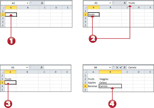
The quickest and easiest way to get data into Excel is to enter the data via the keyboard. You can enter data into a blank worksheet or add data to an existing worksheet. For example, you can enter in the word fruits in cell A2 and press the Enter key.
![]()
![]() Click the cell you want to edit, making it active.
Click the cell you want to edit, making it active.
![]() Enter some data (in this case, Fruits) in the cell. As you type, the data will also show in the Edit bar.
Enter some data (in this case, Fruits) in the cell. As you type, the data will also show in the Edit bar.
![]() Press the Enter key when your edit has been made. Excel makes the cell below (the one you just edited) the active cell.
Press the Enter key when your edit has been made. Excel makes the cell below (the one you just edited) the active cell.
![]() Enter some data into a few different cells, pressing the arrow keys to move around.
Enter some data into a few different cells, pressing the arrow keys to move around.
![]()
Tip: Correcting Data While Editing
![]()
If you make a mistake while entering data, simply press the Backspace key to delete all or a portion of your entry and enter the correct data.
Editing and Deleting Existing Data
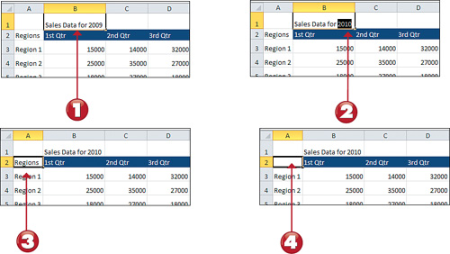
You can always replace a cell’s contents with new data. This comes in handy when you need to correct typing errors or when a cell contains the wrong data. You can also easily erase the contents of a cell by using the Delete key. Erasing a cell is useful when you change your mind about the contents after you enter the data in the cell.
![]()
![]() Double-click the cell you want to edit.
Double-click the cell you want to edit.
![]() Edit the portion of data you need changed.
Edit the portion of data you need changed.
![]() To delete a value, click on the target cell.
To delete a value, click on the target cell.
![]() Press the Delete button on your keyboard.
Press the Delete button on your keyboard.
![]()
Tip: Use Your Arrow Keys
![]()
You can press the left and/or right arrow keys on your keyboard to move the insertion point where you want to make changes.
Zooming Into Your Data
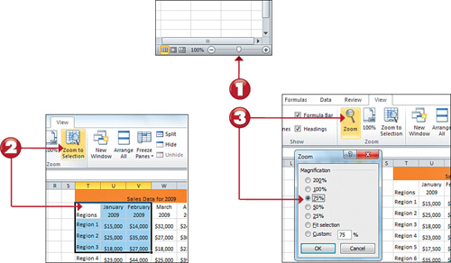
If you want to zoom in and get a closer look at data in your worksheet, you can select a higher percentage of magnification. On the other hand, if you want to zoom out so more of the worksheet shows on the screen at one glance, select a lower percentage of magnification. Excel 2010 provides several ways to zoom in and out.
![]()
![]() Slide the Zoom Slider on the lower-right corner of Excel. Watch your worksheet increase and reduce in magnification as you slide.
Slide the Zoom Slider on the lower-right corner of Excel. Watch your worksheet increase and reduce in magnification as you slide.
![]() Select a Range and choose the Zoom to Selection command on the View tab. Note how Excel automatically increases or reduces magnification so that only that selection is visible.
Select a Range and choose the Zoom to Selection command on the View tab. Note how Excel automatically increases or reduces magnification so that only that selection is visible.
![]() Select the Zoom command on the View tab, then choose your desired magnification. After you click the OK button, observe how Excel applies your zoom preference.
Select the Zoom command on the View tab, then choose your desired magnification. After you click the OK button, observe how Excel applies your zoom preference.
![]()
Tip: Zoom with your Mouse Wheel
![]()
You can use your mouse wheel as another quick way to zoom. Hold down the Ctrl key on your keyboard while you spin your mouse wheel. This increases or reduces magnification depending on the direction you spin (up or down).
Undoing and Redoing Changes
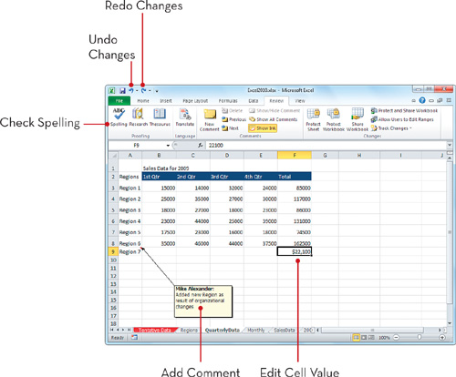
If you make a mistake while working on your spreadsheet and you detect your error immediately, you can undo your action. In addition, if you undo an action by mistake, you can use Excel to quickly redo it.
![]()
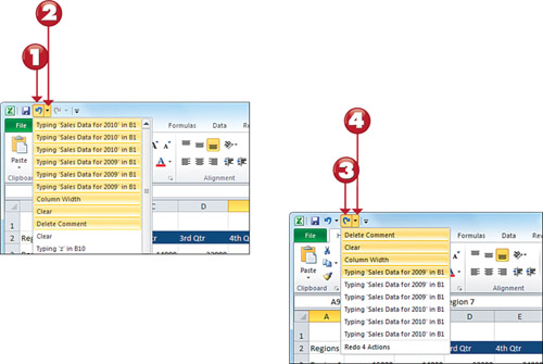
![]() To undo your most recent action, simply click the Undo icon on the Quick Access Toolbar.
To undo your most recent action, simply click the Undo icon on the Quick Access Toolbar.
![]() Click on the drop-down button next to the Undo icon to undo all actions to a certain point.
Click on the drop-down button next to the Undo icon to undo all actions to a certain point.
![]() To redo your most recent action, simply click the Redo icon on the Quick Access Toolbar.
To redo your most recent action, simply click the Redo icon on the Quick Access Toolbar.
![]() Click on the drop-down button next to the Redo icon to redo all actions to a certain point.
Click on the drop-down button next to the Redo icon to redo all actions to a certain point.
![]()
Tip: Using Keyboard Shortcut Keys
![]()
A quick and easy way to undo an action is to use the Ctrl+Z shortcut. Simply hold down the Ctrl key while pressing the Z key. You can redo an action using the Ctrl+Y shortcut.
Copying and Pasting Data
You can avoid the trouble of retyping duplicate information in a worksheet by cutting or copying data from one part of worksheet to another. For example, if you need to duplicate a column of data, there is no need to retype that data. You can copy the data and paste it where you need it. If you want to move the column, you can cut it from its location and paste it to a new location.
![]()
![]() To copy and paste, click the first cell in the range you want to copy and then drag down to highlight the entire range.
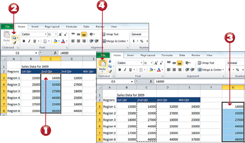
To copy and paste, click the first cell in the range you want to copy and then drag down to highlight the entire range.
![]() Click the Copy command on the Home tab.
Click the Copy command on the Home tab.
![]() Click the cell to which you want the range to be pasted.
Click the cell to which you want the range to be pasted.
![]() Click the Paste command on the Home tab. Excel duplicates your range.
Click the Paste command on the Home tab. Excel duplicates your range.

![]() To copy and paste, click the first cell in the range you want to copy and then drag down to highlight the entire range.
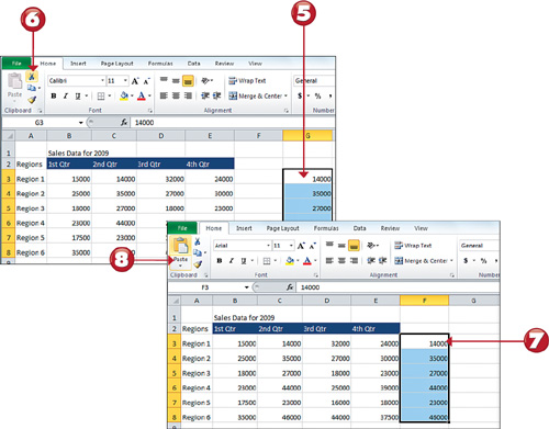
To copy and paste, click the first cell in the range you want to copy and then drag down to highlight the entire range.
![]() Click the Cut command on the Home tab.
Click the Cut command on the Home tab.
![]() Click the cell you want the range pasted to.
Click the cell you want the range pasted to.
![]() Click the Paste command on the Home tab. Excel moves your range.
Click the Paste command on the Home tab. Excel moves your range.
![]()
Tip: Using Keyboard Shortcut Keys
![]()
A quick and easy way to copy and paste data is to use the Ctrl+C and Ctrl+V shortcuts. Hold down the Ctrl key while pressing the C key to copy. Then hold down the Ctrl key while pressing the V key to paste. To cut and paste, you can use the Ctrl+X and Ctrl+V shortcut key combinations.
Freezing Rows and Columns
You might create worksheets that are so large that you cannot view all your data on the screen at the same time. In addition, if you have added row or column labels and you scroll down or to the right, you’ll lose sight of your labels and which data field you’re reviewing. For example, if you are reviewing sales data in columns E and F, it would be nice to see the row title of the cells you are referencing. To help, you can freeze the heading rows and columns so that they’re always visible.
![]()
![]() Click in the cell below the row you want to freeze.
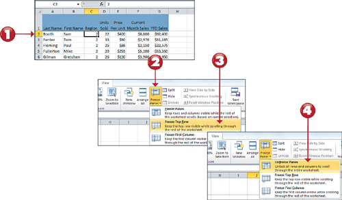
Click in the cell below the row you want to freeze.
![]() On the View tab, click the Freeze Panes command.
On the View tab, click the Freeze Panes command.
![]() Click Freeze Top Row. At this point, you will be able to scroll down and still see the first row of your data table.
Click Freeze Top Row. At this point, you will be able to scroll down and still see the first row of your data table.
![]() To unfreeze the panes, go back to the Freeze Panes command and click the Unfreeze Panes command.
To unfreeze the panes, go back to the Freeze Panes command and click the Unfreeze Panes command.
![]()
Tip: Freezing a Column
![]()
If you are freezing a column, click the cell to the right of the column you want to freeze. Then follow the steps outlined here, but select the Freeze First Column command.
Splitting a Worksheet
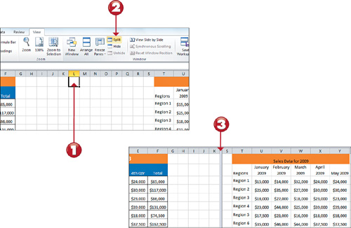
By splitting a worksheet, you can scroll independently into different horizontal and vertical parts of a worksheet. This is useful if you want to view different parts of a worksheet or copy and paste between different areas of a large worksheet.
![]()
![]() Click in the cell where you want to split the worksheet.
Click in the cell where you want to split the worksheet.
![]() On the View tab, click the Split command. You will now see a split bar separating your worksheet into two independently scrollable sections.
On the View tab, click the Split command. You will now see a split bar separating your worksheet into two independently scrollable sections.
![]() Move through the worksheet and see how easily you can simultaneously view other parts of the worksheet.
Move through the worksheet and see how easily you can simultaneously view other parts of the worksheet.
![]()

Inserting Cells
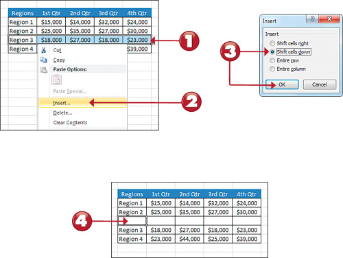
There might be times when you need to insert new cells into the middle of your dataset. For example, if you have a table that shows data by region, you might need to insert blank cells to accommodate a new region. To avoid retyping all the data again or copying and pasting, you can insert cells and shift the current cells to their correct locations.
![]()
![]() Select the cell or cells that need to be shifted to insert new cells.
Select the cell or cells that need to be shifted to insert new cells.
![]() Right-click and choose the Insert option.
Right-click and choose the Insert option.
![]() In the Insert dialog box, choose whether you want to shift existing cells right or down to make room for the new cells. Then press the OK button.
In the Insert dialog box, choose whether you want to shift existing cells right or down to make room for the new cells. Then press the OK button.
![]() Click in your newly created cells and start adding data.
Click in your newly created cells and start adding data.
![]()
Caution: Watch for Misaligned Data When Inserting Cells

Be aware that when you insert a cell, the cells below or to the right of that cell shift (one row down or one column to the right). Be careful that when this happens, your data table does not become misaligned. If it does, you may want to use the Insert Rows or Insert Columns options (explained later in this chapter).
Deleting Cells
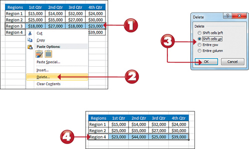
As you work with worksheets, you might find that data needs to be eliminated to keep the worksheet up to date. You can easily delete extraneous cells and shift existing cells to their correct locations.
![]()
![]() Select the cell or cells that need to be deleted.
Select the cell or cells that need to be deleted.
![]() Right-click and choose the Delete option.
Right-click and choose the Delete option.
![]() In the Delete dialog box, choose whether you want to shift existing cells left or up to fill the empty space left by the deleted cells. Press the OK button.
In the Delete dialog box, choose whether you want to shift existing cells left or up to fill the empty space left by the deleted cells. Press the OK button.
![]() Observe that Excel has deleted the specified cells.
Observe that Excel has deleted the specified cells.
![]()
Caution: Watch for Misaligned Data When Deleting Cells

Be aware that when you delete a cell, the cells below or to the right of that cell shift (one row up or one column to the left). Be careful that when this happens, your data table does not become misaligned. If it does, you may want to use the Delete Rows or Delete Columns options (explained later in this chapter).
Inserting and Deleting Rows
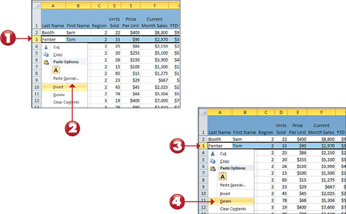
You can insert extra rows into a worksheet to make more room for additional data or formulas. Adding more rows, which gives the appearance of adding space between rows, can also make the worksheet easier to read. Alternatively, you can delete rows from a worksheet to close up some empty space or remove unwanted information.
![]()
![]() Right-click on the row number of the existing row where you want to insert a new row.
Right-click on the row number of the existing row where you want to insert a new row.
![]() Click the Insert option. Excel automatically adds a new row.
Click the Insert option. Excel automatically adds a new row.
![]() To delete a row, right-click on the row number of the existing row that you want deleted.
To delete a row, right-click on the row number of the existing row that you want deleted.
![]() Click the Delete option. Excel automatically removes the specified row.
Click the Delete option. Excel automatically removes the specified row.
![]()
Tip: Hide Rows instead of Delete Rows
![]()
If there is a chance you will need the rows you are deleting, another alternative is to leave them intact—only hidden. Hide them by selecting your rows, right-clicking, and then selecting the Hide option. This way, the rows will not be visible, but you can always get them back by unhiding them.
Inserting and Deleting Columns
You can insert extra columns into a worksheet to make room for more data or formulas. Adding more columns, which gives the appearance of adding space between columns, can also make the worksheet easier to read. Alternatively, you might want to delete columns from a worksheet to close up some empty space or remove unwanted information.
![]()
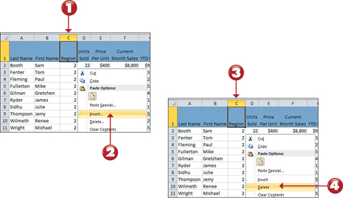
![]() Right-click on the column letter of the existing column where you want to insert a new column.
Right-click on the column letter of the existing column where you want to insert a new column.
![]() Click the Insert option. Excel automatically adds a new column.
Click the Insert option. Excel automatically adds a new column.
![]() To delete a column, right-click on the column number of the existing column that you want deleted.
To delete a column, right-click on the column number of the existing column that you want deleted.
![]() Click the Delete option. Excel automatically removes the specified column.
Click the Delete option. Excel automatically removes the specified column.
![]()
Tip: Hide Columns instead of Delete Columns
![]()
You can always hide your columns instead of deleting them for good. This way, you can always get them back simply by unhiding them. Select the columns you want to hide, right-click, and then select the Hide option. To unhide, select the columns to the left and right of the hidden columns, right-click, and then select the Unhide option.
Moving Data
Excel lets you move information from one cell into another cell, which means you do not have to type the data into the new cell and then erase the data in the old location. You might want to move data in a worksheet because the layout of the worksheet has changed.
![]()
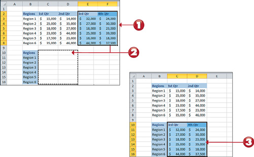
![]() Select the cells you want to move.
Select the cells you want to move.
![]() Click the border of the selected cells and drag the cells to the location in the worksheet where you want to move the data.
Click the border of the selected cells and drag the cells to the location in the worksheet where you want to move the data.
![]() Observe that Excel has moved your data.
Observe that Excel has moved your data.
![]()
Note: Moving vs Cutting and Pasting
![]()
Moving data is essentially the same action as cutting and pasting data. That is, both actions allow you to move large chunks of data from one location to another. But you would typically “move” data when you need to move the data a short distance and don’t want to take your hand off the mouse.

Finding Data
You will often encounter situations where you will need to find specific information in a large spreadsheet. For example, suppose you want to quickly find the row that shows the sales information for Jerry Thompson. Instead of scanning each row for the data you need, which can be time consuming, you can use Excel’s Find feature.
![]()
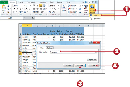
![]() On the Home tab, click Find and Select, and then click Find or press shortcut key Ctrl+F.
On the Home tab, click Find and Select, and then click Find or press shortcut key Ctrl+F.
![]() In the Find What text box, enter the data you want to find.
In the Find What text box, enter the data you want to find.
![]() Click the Find Next button. Excel finds the first instance of the data you typed and makes the cell that contains it the active cell. You can click the Find Next button to search for the next instance.
Click the Find Next button. Excel finds the first instance of the data you typed and makes the cell that contains it the active cell. You can click the Find Next button to search for the next instance.
![]() Click the Close button when you are done searching.
Click the Close button when you are done searching.
![]()
Tip: Finding All Instances
![]()
Click the Find All button in the Find and Replace dialog box to view a list, complete with cell locations and worksheet tab names, of all the instances of the data you entered in the Find What text box. While there, you can press Ctrl+A to have Excel select all the cells in that list.
Replacing Data
Imagine that you discover some data in your table in which a company’s name has been consistently misspelled, or that a salesperson you reference in a data table has changed his last name. You definitely would not want to find and replace all that data manually. Fortunately, Excel enables you to search for instances of incorrect or outdated data and replace it with new data using its Find and Replace feature.
![]()
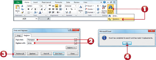
![]() On the Home tab, click Find and Select and then click Replace.
On the Home tab, click Find and Select and then click Replace.
![]() In the Find What text box, type the data you would like to find. Press the Tab key to move the cursor to the Replace With text box, and type the replacement data.
In the Find What text box, type the data you would like to find. Press the Tab key to move the cursor to the Replace With text box, and type the replacement data.
![]() Click Replace All to replace all instances of the data you typed. (Alternatively, click Find Next to find the first instance of the data and click Replace to replace it.)
Click Replace All to replace all instances of the data you typed. (Alternatively, click Find Next to find the first instance of the data and click Replace to replace it.)
![]() Excel notifies you of the number of replacements it made. Click OK.
Excel notifies you of the number of replacements it made. Click OK.
![]()
Tip: Narrowing Your Search Criteria
![]()
Clicking on the Options button on the Find and Replace dialog box reveals a few options you can use to make search criteria more specific. To conduct a case-sensitive search (for example, finding all instances of “Thompson” but not “thompson”), choose the Match Case option. Choose Match Entire Cell Contents to limit your search to cells that contain no more and no less than the data you type.
Applying a Data Filter
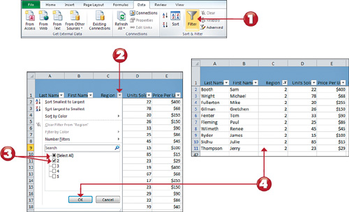
When working with a large data table, it is sometimes useful to filter the table so that you can only see or work with a specific set of records. For instance, let’s say you only want to see the sales reps in Region 2. When you want to work with a subset of records, you can use Excel’s Filter. The Filter function allows you to see only those records that meet the criteria you select.
![]()
![]() Click on the Filter command on the Data tab.
Click on the Filter command on the Data tab.
![]() You will immediately see filter drop-downs inside each of your header columns. Click on the drop-down selector for the column you want to filter.
You will immediately see filter drop-downs inside each of your header columns. Click on the drop-down selector for the column you want to filter.
![]() Click the (Select All) option to clear all the check boxes, then click the check box next to the value by which you want to filter.
Click the (Select All) option to clear all the check boxes, then click the check box next to the value by which you want to filter.
![]() Click the OK button to apply the filter. Observe the funnel icon on the filtered column, indicating a filtered state.
Click the OK button to apply the filter. Observe the funnel icon on the filtered column, indicating a filtered state.
![]()
Tip: Removing Data Filter Drop-downs
![]()
To remove the data filter drop-downs, simply go to the Data tab and select the Filter command. This clears all filters and eliminates the drop-downs from your header labels.
Sorting Data
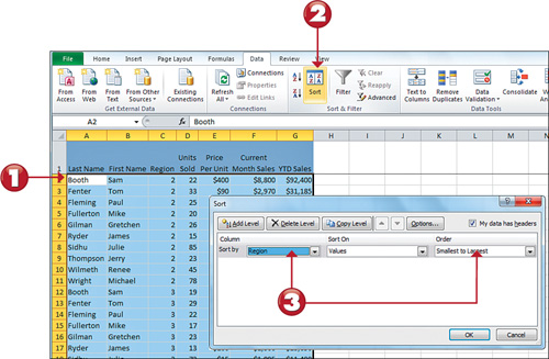
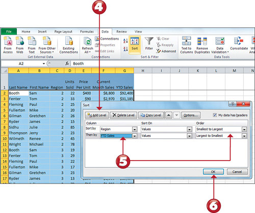
You will often want to change the ordering of your data. For example, you might want to sort a table of sales reps by their regions, then by YTD sales. You can meet this need by using Excel’s Sort function.
![]()
![]() Click on any cell within the data table you are going to sort.
Click on any cell within the data table you are going to sort.
![]() On the Data tab, click the Sort command.
On the Data tab, click the Sort command.
![]() The Sort Dialog box opens. Select the field you want to sort and then specify whether you want to sort Smallest to Largest or Largest to Smallest.
The Sort Dialog box opens. Select the field you want to sort and then specify whether you want to sort Smallest to Largest or Largest to Smallest.

![]() Click the Add Level button to add another level of sorting.
Click the Add Level button to add another level of sorting.
![]() Select another field to sort by, then specify whether you want to sort Smallest to Largest or Largest to Smallest.
Select another field to sort by, then specify whether you want to sort Smallest to Largest or Largest to Smallest.
![]() After you click the OK button, Excel immediately applies your custom sort.
After you click the OK button, Excel immediately applies your custom sort.
![]()

Adding and Managing Cell Comments
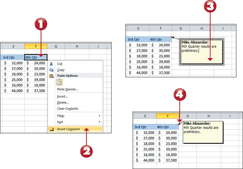
Some cells contain data that requires an explanation or special attention. Comments provide a way to attach this type of information to individual cells without cluttering the cells with extraneous information. A red triangle indicates that a cell contains a comment, which you can view in several different ways. After a comment is in place, Excel makes it easy to edit or delete it.
![]()
![]() Right-click the cell to which you want to add a comment.
Right-click the cell to which you want to add a comment.
![]() Select Insert Comment.
Select Insert Comment.
![]() Type the desired text into the comment area. When you’re finished, click anywhere in the worksheet to accept the comment.
Type the desired text into the comment area. When you’re finished, click anywhere in the worksheet to accept the comment.
![]() The cell’s upper-right corner now contains a red triangle, indicating the presence of a comment. To view the comment, hover the mouse pointer over the triangle.
The cell’s upper-right corner now contains a red triangle, indicating the presence of a comment. To view the comment, hover the mouse pointer over the triangle.
Tip: Display Comments Without Hovering
![]()
You can make Excel display a cell’s comments without the need to hover over the cell. To do so, right-click the commented cell and select Show/Hide Comments. To re-hide the comment, right-click the commented cell and select Hide Comment.
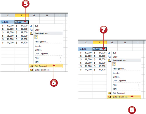
![]() To edit a comment, right-click on the commented cell.
To edit a comment, right-click on the commented cell.
![]() Select the Edit Comment option.
Select the Edit Comment option.
![]() To delete a comment, right-click on the commented cell.
To delete a comment, right-click on the commented cell.
![]() Select the Delete Comment option.
Select the Delete Comment option.
![]()


