Chapter 1. Working with the Excel User Interface
The Ribbon User Interface
For those of you who have worked with Microsoft Excel 2003, the first thing you will notice when using Microsoft Excel 2010 is that Microsoft has done away with the standard toolbar. That is, you don’t see the typical pull-down menus found in older versions of Word, PowerPoint, and Excel. Instead, you’ll see the interface dubbed the Ribbon.
The Ribbon was actually introduced with the Release of Office 2007 as a significant departure from the old way of selecting commands. Instead of having to drill into multiple levels of toolbars to find the command that you need, the Ribbon brings your favorite commands out into the open and even allows you to discover some new commands you never knew existed.
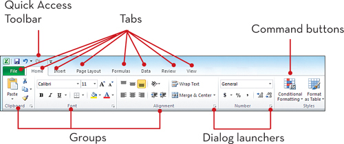
The Ribbon is made up of five basic components: the Quick Access Toolbar, tabs, groups, command buttons, and dialog launchers. The Quick Access Toolbar is essentially a customizable toolbar that allows you to add commands that are most important to your daily operations. Tabs contain groups of commands that are loosely related to core tasks. In fact, it helps to think of each tab as a theme. Groups contain sets of commands that fall under the umbrella of that tab’s core task. Each group contains commands buttons, which are objects you click to select the action you want to execute. Dialog launchers are located in the lower-right corner of certain groups. Clicking on any one of these activates a dialog box containing the full spectrum of options for a given group.

The Anatomy of the Ribbon Interface
Familiarizing Yourself with the Ribbon Tabs
Each tab in the Ribbon contains groups of commands that are loosely related to a central task. Don’t be alarmed by the number of commands on each tab. As you go through this book, you’ll quickly become familiar with each of the common Excel commands. For now, take some time to get familiar with each of Excel’s default tabs.
![]()
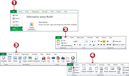
![]() Click the File tab. This tab contains all the higher-level Excel commands, such as open, save, print, and close.
Click the File tab. This tab contains all the higher-level Excel commands, such as open, save, print, and close.
![]() Click the Home tab. This tab contains commands for common actions such as formatting, copying, pasting, inserting, and deleting columns and rows.
Click the Home tab. This tab contains commands for common actions such as formatting, copying, pasting, inserting, and deleting columns and rows.
![]() Click the Insert tab. This tab contains commands that allow you to insert objects such as charts and shapes into your spreadsheets.
Click the Insert tab. This tab contains commands that allow you to insert objects such as charts and shapes into your spreadsheets.
![]() Click the Page Layout tab. This tab holds all the commands that allow you to determine how your spreadsheet looks, both onscreen and when printed.
Click the Page Layout tab. This tab holds all the commands that allow you to determine how your spreadsheet looks, both onscreen and when printed.
![]() Click the Formulas tab. This tab holds all the commands that help define, control, and audit Excel formulas.
Click the Formulas tab. This tab holds all the commands that help define, control, and audit Excel formulas.
![]() Click the Data tab. This tab features commands that allow you to connect to external data, as well as manage the data in your spreadsheet.
Click the Data tab. This tab features commands that allow you to connect to external data, as well as manage the data in your spreadsheet.
![]() Click the Review tab. With commands such as Spell Check, Protect Sheet, Protect Workbook, and Track Changes, the theme of the Review tab is protecting data integrity in your spreadsheet.
Click the Review tab. With commands such as Spell Check, Protect Sheet, Protect Workbook, and Track Changes, the theme of the Review tab is protecting data integrity in your spreadsheet.
![]() Click the View tab. The commands on this tab are designed to help you control how you visually interact with your spreadsheet.
Click the View tab. The commands on this tab are designed to help you control how you visually interact with your spreadsheet.
![]()
Tip: Minimizing the Ribbon
![]()
If you feel the Ribbon takes up too much space at the top of your screen, you can minimize (hide) it. Right-click on the Ribbon and select Minimize the Ribbon. At this point, the Ribbon only becomes visible if you click on a tab. To revert back to the default Ribbon view, right-click the Ribbon and click Minimize the Ribbon again.
Understanding Contextual Tabs
Contextual tabs are special types of tabs that appear only when a particular object is selected, such as a chart or a shape. These contextual tabs contain commands that are specific to whatever object has the current focus.
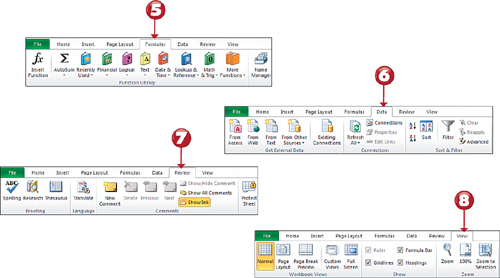
To see a contextual tab in action, add a shape to a spreadsheet. After a shape has been added, a new Format tab appears. This is not a standard tab, but a contextual tab—meaning it only activates when you are working with a shape.
You can follow the steps in this walkthrough to add a shape. Shapes and other graphics are covered in detail in Chapter 7, “Working with Graphics.”
![]()
![]() Click the Insert tab.
Click the Insert tab.
![]() Click the Shapes command button.
Click the Shapes command button.
![]() Select the rectangle shape.
Select the rectangle shape.
![]() Click anywhere on your spreadsheet to embed your selected shape.
Click anywhere on your spreadsheet to embed your selected shape.
![]() Click on your shape and note the Contextual tab that appears each time the shape is activated.
Click on your shape and note the Contextual tab that appears each time the shape is activated.
![]()

Understanding Workbooks and Worksheets
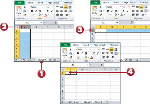
An Excel file, often referred to as a workbook, contains one or more spreadsheets, or worksheets. Each box in the worksheet area is referred to as a cell. Each cell has a cell address, which is comprised of a column reference and a row reference. The letters going across the top of the worksheet make up the column reference. The numbers going down the left side of the worksheet make up the row reference. For example, the address of the top, leftmost cell is A1. This is because the cell is located at the intersection of the A column and row 1.
![]()
![]() Click a worksheet’s tab to view that worksheet’s area.
Click a worksheet’s tab to view that worksheet’s area.
![]() Click the column reference and observe how the entire column is selected.
Click the column reference and observe how the entire column is selected.
![]() Click the row reference and observe how the entire row is selected.
Click the row reference and observe how the entire row is selected.
![]() Click the cell intersecting at column A and row 1. Notice how you can select a single cell on the worksheet area.
Click the cell intersecting at column A and row 1. Notice how you can select a single cell on the worksheet area.
![]()
Note: The Big Grid
![]()
Excel 2010 has 1,048,576 rows and 16,384 columns. This means that there are more than 17 billion cells in a single Excel worksheet. So what happens if you need more than a million rows and more than 16,000 columns? Well, the answer is that you’ll have to start a new worksheet.
Customizing the Quick Access Toolbar
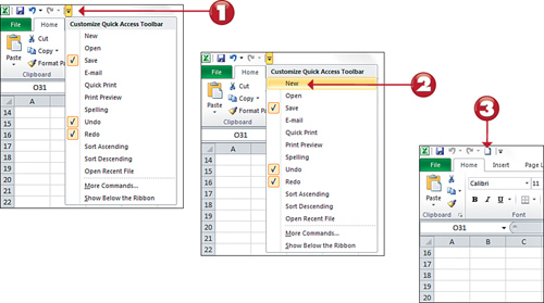
By default, the Quick Access Toolbar contains three commands: Save, Undo, and Redo. If you click on the drop-down selection next to the Quick Access Toolbar, you’ll see that these three commands are only three of eleven that are available as pre-built or built-in options. Placing a check next to any of the options that you see here automatically adds each option to the Quick Access Toolbar. So, clicking New adds the New command, and clicking Open adds the Open command. You can literally click each one of these and have all these pre-built options available to you in the Quick Access Toolbar.
![]()
![]() Click the Quick Access Toolbar drop-down to see all the commands you can add.
Click the Quick Access Toolbar drop-down to see all the commands you can add.
![]() Click the New pre-built command to add it to the Quick Access Toolbar.
Click the New pre-built command to add it to the Quick Access Toolbar.
![]() Note that you now have a new icon on your Quick Access Toolbar.
Note that you now have a new icon on your Quick Access Toolbar.
![]()
Note: Moving the Quick Access Toolbar
![]()
You can move the Quick Access Toolbar under the Ribbon by right-clicking its dropdown and selecting Show Below the Ribbon.
Adding Commands to the Quick Access Toolbar
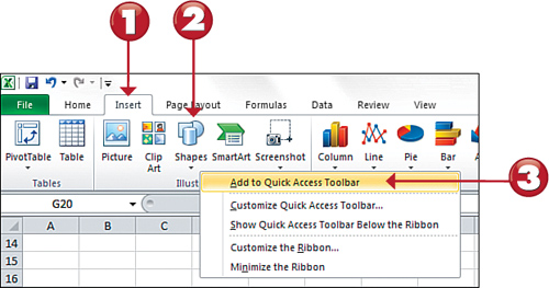
You’re not limited to the commands shown on the Quick Access Toolbar—you can add all kinds of commands. For example, if you often work with shapes, you can add the Shapes command to the Quick Access Toolbar.
![]()
![]() Click the Insert tab.
Click the Insert tab.
![]() Right-click the Shapes command button.
Right-click the Shapes command button.
![]() Select Add to Quick Access Toolbar.
Select Add to Quick Access Toolbar.
![]()
Tip: Adding Entire Groups
![]()
You can add entire groups to your Quick Access Toolbar. For instance, if you often use the Illustrations group on the Insert tab, you can right-click on that entire group and click Add to Quick Access Toolbar.
Adding Hidden Commands to the Quick Access Toolbar
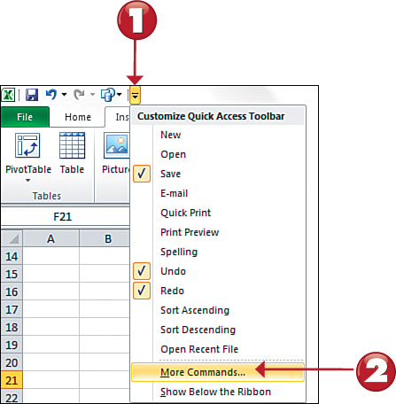
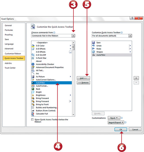
A closer look at the drop-down menu next to the Quick Access Toolbar reveals a command called More Commands. If you select this, the Excel options dialog box opens up with the Quick Access Toolbar panel activated. This panel allows you to select from the entire menu of Excel commands, adding them to your Quick Access Toolbar. This comes in handy if you want to add some of the more obscure Excel commands that aren’t found in the Ribbon.
![]()
![]() Click the Quick Access Toolbar drop-down.
Click the Quick Access Toolbar drop-down.
![]() Select the More Commands option.
Select the More Commands option.

![]() Choose Commands Not in the Ribbon.
Choose Commands Not in the Ribbon.
![]() Find and select the AutoFilter command.
Find and select the AutoFilter command.
![]() Click the Add button.
Click the Add button.
![]() Click the OK button to add the command to the Quick Access Toolbar.
Click the OK button to add the command to the Quick Access Toolbar.
![]()
