
Hypothesis tests
Abstract
Hypothesis testing grew out of quality control, when it was necessary to decide to accept or reject a batch of items based on a relatively small number of tested items. Today, when quality control engineers decide what sample size to take for a reliable inference about the entire product batch or when they need to check the significance of the differences between two separate tests, or in many other cases, they use various statistical tests to obtain the technically correct solution. This chapter describes the test commands available in the hypothesis tests section of the Statistics Toolbox™ together with their applications for use in QA. A basic familiarity with statistics and probability theory is assumed.
6.1 Hypothesis testing outlines
A variety of tests may be conducted using the same steps: first, a tested hypothesis is stated, then an analysis plan is formulated, the sample data is analyzed, and finally, the decision is made to accept or reject the null hypothesis.
Hypothesis
In this stage, two mutually exclusive hypotheses are stated: a null and an alternative. They should be formulated so that if one is true then the other must be false.
Analysis plan
The following elements should be specified:
■ The significance level a, frequently chosen to be equal to 0.05 or 0.01.
■ The test method and test type, which involve a sample of the data statistics and a sample of the distribution.
■ The assessed probability associated with the test statistic. In cases when the test probability is less than the significance level, the null hypothesis should be rejected.
Sample data analysis
Now, calculations of the sample statistics are performed in order to summarize the sample. This statistic varies according to the test type, but its distribution under the null hypothesis must be known or assumed. After achieving results, the probability of observing a sample statistic, called p-value, is defined.
Decision
Finally, a comparison of the p-value with the significance level should be executed; when the P-value is less than the significance level, the null hypothesis is rejected. The significance level α is the probability of rejecting the null hypothesis when it is actually true - a Type I error. However, even if the null hypothesis is not rejected, it may still be false - a Type II error. Thus, it is sound reasoning to check the alternative hypothesis. The distribution of the test statistic under the alternative hypothesis determines the probability β of a Type II error (which often occurs due to small sample sizes). The probability to correctly reject a false null hypothesis called the power of the test and is 1 - β.
The Statistics Toolbox™ includes various different test commands connected to the selected test type. These commands analyze the sample data and provide the answer - whether the null hypothesis is true or false. Therefore, the steps taken to analyze sample data and the decision to reject a null hypothesis or not are a function of the available test commands. However, before testing, it is necessary to select the commands suitable to the problem. The existing tests are divided into two categories: parametric and nonparametric. The parametric statistical test makes assumptions about the parameters of the distribution from which one's data are drawn, while the non-parametric test makes no such assumptions. Correspondingly, some of the available test commands in the Statistics Toolbox™ recognize parametric tests, for example, the Jarque-Bera, Lilienfors and Kolmogorov-Smirnov tests; others recognize non- parametric tests, for example, Wilcoxon signed-rank and Wilcoxon rank- sum tests. These two groups frequently subdivide into three subgroups each: paired, unpaired and complex (more than two samples) data tests. These concepts and steps for deciding on test selection belong to statistics courses and are out of the scope of this book. The following provides a brief description of test commands and their usage without a grounding of their selection.
6.2 The t-test with the ttest command
This test is used when the sample size is small, and variance or standard deviation of the underlying normal distribution is unknown. It can be applied to one-sample or to paired-sample data (the latter test is often termed pre/post-test); a data set is termed paired when each set has the same number of data points and each point in one data set is related to the appropriate point in the other. Possible forms of the MATLAB® command for this test are
![]()
where x and y are equal vectors with the data of the two samples that are transformed by these commands to the test statistic form ![]() where
where ![]() and s are the sample mean and standard deviation respectively, m is the hypothesized population mean; n is the sample size; alpha is the (100* α)% significance level; h is the output variable that is equal to 1 when the null hypothesis is rejected and is 0 in the other case; and the output ρ-value is the smallest level of significance in which a null hypothesis may be rejected.
and s are the sample mean and standard deviation respectively, m is the hypothesized population mean; n is the sample size; alpha is the (100* α)% significance level; h is the output variable that is equal to 1 when the null hypothesis is rejected and is 0 in the other case; and the output ρ-value is the smallest level of significance in which a null hypothesis may be rejected.
The first of the ttest commands performs a t-test for the null hypothesis when the x-data is normally distributed with mean m and an unknown variance and is compared with the alternative – that the mean is not m. The second ttest command performs a paired-sample t-test for the null hypothesis when the difference x– y is normally distributed with mean 0 and an unknown variance, and is compared with the alternative - that the mean is not zero; x and y must be equivalent vectors. The command can be written without the alpha value, in this case, α = 0.05 by default. The output argument ρ can be omitted in both ttest commands presented here.
Problem: Explain the use of a ttest command for electronic device lifetime test data: 8.6, 10.2, 3.8, 4.9, 19.0, 10.0, 5.4, 4.3, 12.2 and 8.6, in days. Devices of this model should have a mean lifetime of 8.5 days. Is it correct to say that the lifetime data derives from a normal distribution with a mean of 8.5?
The null hypothesis for this problem is that the lifetime data are normally distributed with mean m. The alternative hypothesis is that the mean is not m.
The h = 0 indicates a failure to reject the null hypothesis (the mean is 8.5), h = 1 rejects the null hypothesis (the mean is not 8.5).
The problem is solved using the following commands, written as the Ch6_ttest_Ex script program:
% the paired-sample t-test example
% h = 0: x is from the norm distribution with the m mean
% h = 1: the mean is not m for this data
x = [8.6 10.2 3.8 4.9 19.0 10.0 5.4 4.3 12.2 8.6];
alpha = 0.05; % significance level
m = 8.5; % compared mean
[h,p_value] = ttest(x,m,alpha)
After running this program, the Command Window shows:
> > Ch5_ttest_Ex
h =
0
p_value =
0.8938
Thus, the h = 0 test fails to reject the null hypothesis (the lifetime data derives from the normal distribution with the 8.5 mean) at the default α = 0.05 significance level.
To perform a t-test for two non-paired samples, the ttest2 command is used (see Table 6.1).
Table 6.1
Commands for hypothesis tests
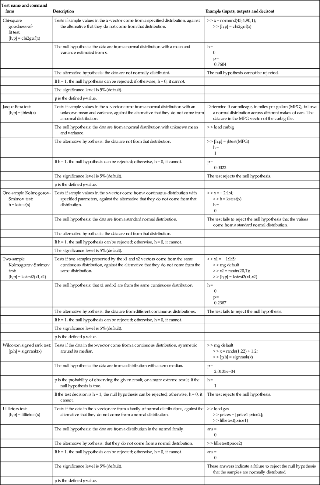
| Test name and command form | Description | Example (inputs, outputs and decison) |
| Chi-square goodness-of- fit test: [h,p] = chi2gof(x) | Tests if sample values in the x -vector come from a specified distribution, against the alternative that they do not come from that distribution. | > > x = normrnd(45,4,90,1); > > [h,p] = chi2gof(x) |
| The null hypothesis: the data are from a normal distribution with a mean and variance estimated from x. | h = 0 p = 0.7604 | |
| The alternative hypothesis: the data are not normally distributed. | The null hypothesis cannot be rejected. | |
| If h = 1, the null hypothesis can be rejected; if otherwise, h = 0, it cannot. | ||
| The significance level is 5% (default). | ||
| p is the defined p-value. | ||
| Jarque-Bera test: [h,p] = jbtest(x) | Tests if sample values in the x -vector come from a normal distribution with an unknown mean and variance, against the alternative that they do not come from a normal distribution. | Determine if car mileage, in miles per gallon (MPG), follows a normal distribution across different makes of cars. The data are in the MPG vector of the carbig file. |
| The null hypothesis: the data are from a normal distribution with unknown mean and variance. | > > load carbig | |
| The alternative hypothesis: the data are not from that distribution. | > > [h,p] = jbtest(MPG) h = 1 | |
| If h = 1, the null hypothesis can be rejected; otherwise, h = 0, it cannot. | p = 0.0022 | |
| The significance level is 5% (default). | The test rejects the null hypothesis. | |
| p is the defined p-value. | ||
| One-sample Kolmogorov-Smirnov test: h = kstest(x) | Tests if sample values in the x-vector come from a continuous distribution with specified parameters, against the alternative that they do not come from that distribution. | > > x = − 2:1:4; > > h = kstest(x) h = 0 |
| The null hypothesis: the data are from a standard normal distribution. | The test fails to reject the null hypothesis that the values come from a standard normal distribution. | |
| The alternative hypothesis: the data are not from that distribution. | ||
| If h = 1, the null hypothesis can be rejected; otherwise, h = 0, it cannot. | ||
| The significance level is 5% (default). | ||
| Two-sample Kolmogorov-Smirnov test: [h,p] = kstest2(x1,x2) | Tests if two samples presented by the x1 and x2 vectors come from the same continuous distribution, against the alternative that they do not come from the same distribution. | > > x1 = − 1:1:5; > > rng default > > x2 = randn(20,1); > > [h,p] = kstest2(x1,x2) |
| The null hypothesis: that x1 and x2 are from the same continuous distribution. | h = 0 p = 0.2387 | |
| The alternative hypothesis: the data are from different continuous distributions. | The test fails to reject the null hypothesis. | |
| If h = 1, the null hypothesis can be rejected; otherwise, h = 0, it cannot. | ||
| The significance level is 5% (default). | ||
| p is the defined p-value. | ||
| Wilcoxon signed rank test: [p,h] = signrank(x) | Tests if the data in the x-vector come from a continuous distribution, symmetric around its median. | > > rng default > > x = randn(1,22) + 1.2; > > [p,h] = signrank(x) |
| The null hypothesis: the data are from a distribution with a zero median. | p = 2.0135e–04 | |
| p is the probability of observing the given result, or a more extreme result, if the null hypothesis is true. | h = 1 | |
| If the test decision is h = 1, the null hypothesis can be rejected; otherwise, h = 0, it cannot. | The test rejects the null hypothesis. | |
| Lilliefors test: [h,p] = lillietest(x) | Tests if the data in the x-vector are from a family of normal distributions, against the alternative that they do not come from a normal distribution. | > > load gas > > prices = [price1 price2]; > > lillietest(price1) |
| The null hypothesis: the data are from a distribution in the normal family. | ans = 0 | |
| The alternative hypothesis: that they do not come from a normal distribution. | > > lillietest(price2) | |
| If h = 1, the null hypothesis can be rejected; otherwise, h = 0, it cannot. | ans = 0 | |
| The significance level is 5% (default). | These answers indicate a failure to reject the null hypothesis that the samples are normally distributed. | |
| p is the defined p-value. | ||
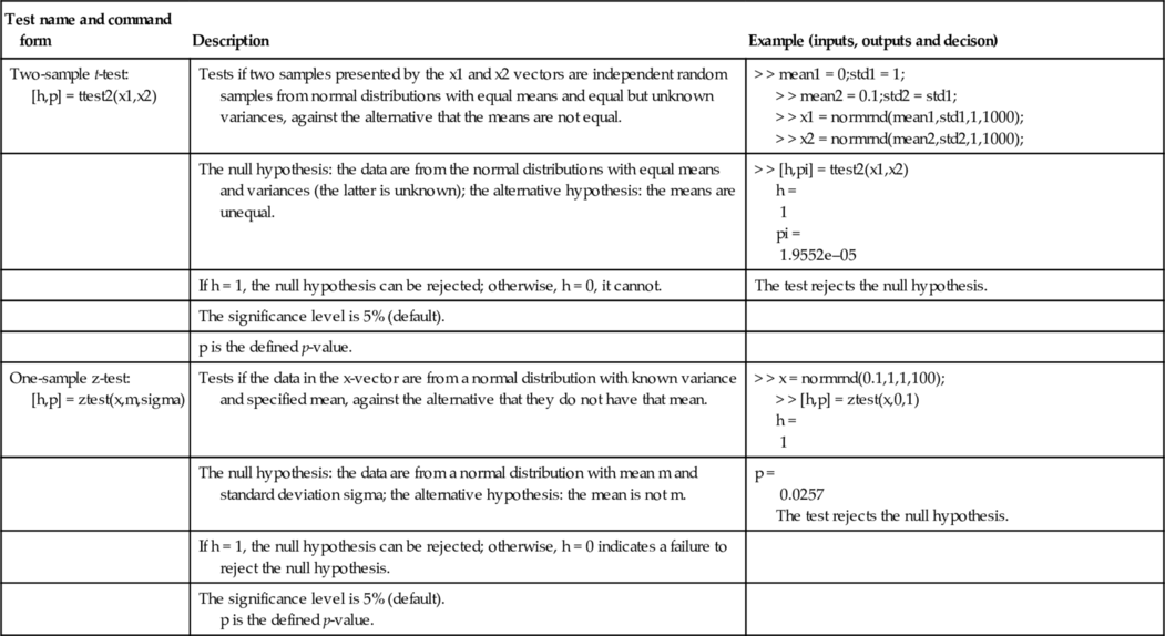
| Two-sample t-test: [h,p] = ttest2(x1,x2) | Tests if two samples presented by the x1 and x2 vectors are independent random samples from normal distributions with equal means and equal but unknown variances, against the alternative that the means are not equal. | > > mean1 = 0;std1 = 1; > > mean2 = 0.1;std2 = std1; > > x1 = normrnd(mean1,std1,1,1000); > > x2 = normrnd(mean2,std2,1,1000); |
| The null hypothesis: the data are from the normal distributions with equal means and variances (the latter is unknown); the alternative hypothesis: the means are unequal. | > > [h,pi] = ttest2(x1,x2) h = 1 pi = 1.9552e–05 | |
| If h = 1, the null hypothesis can be rejected; otherwise, h = 0, it cannot. | The test rejects the null hypothesis. | |
| The significance level is 5% (default). | ||
| p is the defined p-value. | ||
| One-sample z-test: [h,p] = ztest(x,m,sigma) | Tests if the data in the x-vector are from a normal distribution with known variance and specified mean, against the alternative that they do not have that mean. | > > x = normrnd(0.1,1,1,100); > > [h,p] = ztest(x,0,1) h = 1 |
| The null hypothesis: the data are from a normal distribution with mean m and standard deviation sigma; the alternative hypothesis: the mean is not m. | p = 0.0257 The test rejects the null hypothesis. | |
| If h = 1, the null hypothesis can be rejected; otherwise, h = 0 indicates a failure to reject the null hypothesis. | ||
| The significance level is 5% (default). p is the defined p-value. |
6.3 Wilcoxon rank sum test
This test is sometimes termed the Mann–Whitney U test and is used in non-parametric hypothesis testing, when two independent unequal- sized samples have to be compared to verify their identity. This method does not require any assumptions about the distribution function and is non-parametric. The command for this test takes the form
![]()
where x and y are the vectors with the data of two independent samples; the length of the x and y vectors can be different; 'alpha' is the name of the significance level, α, and alfa_value is the values of α; p is the p-value; and h is the test decision.
Here, the null hypothesis is that the samples are from a continuous distribution with the same median. The alternative hypothesis is that they are not.
If p < α then the null hypothesis is rejected and h = 1; p > α indicates a failure to reject the null hypothesis and h = 0.
The 'alpha',alfa_value argument pair presents the significant level a; it is optional and can be omitted, in which case α = 0.05 by default.
Problem: Explain the usage of the ranksum command for computer lifetime data, in weeks. The measured lifetimes are 8.6, 10.2, 3.8, 4.9, 19.0, 10.0, 5.4, 4.3, 12.2, 8.6 and 10.1, 9.2, 7.8, 14.5, 16.1, 3.2, 4.9, 8.8, 11.4, 20.2 for the actual and enhanced models respectively. Can we say that the median difference of the pairs is zero? Assume the significance level α is 0.05. The null hypothesis for this is that the median difference in the paired lifetime values is insignificant, h = 0; the alternative is that it is significant, h = 1.
The problem is solved using commands written as the Ch6_Wilcoxon_Ex script program:
% the paired-smaple t-test example
% h = 0:do not reject the null-hypothesis(equal medians)
% h = 1:reject the null-hypothesis
x = [8.6 10.2 3.8 4.9 19.0 10.0 5.4 4.3 12.2 8.6];
y = [10.1 9.2 7.8 14.5 16.1 3.2 4.9 8.8 11.4 20.2];
alpha = 0.05;
[pvalue,h] = ranksum(x,y)
After running the commands:
> > Ch5_Wilcoxon_Ex
pvalue =
0.4053
h =
0
The p -value of the test is greater than the significance level and the null- hypothesis cannot be rejected; thus, the results – h = 0 – means that there is no real lifetime difference.
6.4 Sample size and power of test
The power of the test is in the probability of rejecting the hypothesis when it is actually true. A high power value is desirable (0.7 to 1) as it means that there is a high probability of rejecting the null hypothesis when the null hypothesis is false. The power of the test depends on the sample size, the difference of the variances, the significance level and the difference between the means of the two populations. In MATLAB®, the sampsizepwr command calculates test power and size; it takes the form
![]()
where testtype is the string with the test name; some of the available names are 'z' and 't', for z- and £-test respectively; p0 is a two-element vector [mu0 sigma0] of the mean and standard deviation; p1 is the true mean value; n is the sample size; and power is the defined value of the power of the test.
Let us illustrate the sampsizepwr command with the following example. An agriculturist defines in 10 tests that his agricultural equipment operates 105 min on average to complete an operation with a standard deviation of 10 min. The time stated by a manufacturer is 90 min (taken as the true value). Find if the values of operation time are equal. The mean and standard deviation under the null hypothesis here are 105 and 10 respectively, and 90 here is the mean value using the alternative hypothesis. The commands for defining the problem are
> > n = 10;
> > testtype = 't';
> > p0 = [105, 10]; p1 = 90;
> > power = sampsizepwr(testtype,p0,p1,[],n)
power =
0.9873
Thus in the case of a t-test type, there is a high probability of rejecting the null hypothesis when the null hypothesis is false.
The command that can be used for defining the sample size, appropriate form is:
![]()
Here, the notations are the same as those used in the previous command form. The significance level and tail type can be added in the list of input arguments, for example, n = sampsizepwr(testtype,p0,p1,power,[],'tail',' right'), for further details, see Subsection 6.6.3.
6.5 Supplementary commands for the hypothesis tests
In addition to the test commands described in the previous subsections, the Statistics Toolbox™ provides many other commands for hypothesis tests. Some of these are presented in Table 6.1.
Some of the examples in this table use the carbig and gas files, provided in the Sample Data Sets section of the Statistics Toolbox™ documentation. The files should be loaded by typing the load file_name command; the file_name is one of the files, e.g., carbig. The carbig file contains the 13 vectors/matrices with some of the parameters of different models of cars manufactured in the years 1970–1982. The gas file contains two vectors with two samples of gasoline prices in the state of Massachusetts in 1993, the first vector for a day in January and the second, a day one month later.
The commands written without output parameters display one value only (h or p, corresponding to the test). The non-default significance level can be input in the chi2gof, jbtest, kstest, kstest2, lilietest, and ztest commands, usually just after the input arguments presented in the table, e.g., ztest(x,m,sigma,alpha); for related details type the help command with the appropriate test name in the Command Window. The test commands in the table written for two-tiled tests by default, ztest and ttest2, can be used for the one-tailed tests. In this case, their form is more complicated and outside the scope of this book; the details can be obtained using the help command.
6.6 Application examples
6.6.1 The IQ with the one-sampie z-test
IQ is the intelligence quotient score that measures a person's intelligence and is defined with a standardized test.
Problem: The IQ average for national college students is 113 with standard deviation 14. An IQ test of 12 students of one of the colleges gives the following results: 127, 99, 120, 139, 99, 134, 94, 95, 126, 108, 94, and 90. Are these students the same as the national average? Compose the function that uses the ztest command and displays the result of the hypothesis test.
The null hypothesis, h = 0: the mean IQ is 113 (e.g. the IQ score for all students in the tested college will be 113).
The alternative hypothesis, h = 1: the mean IQ is not equal to 113 (IQ score for all students in the tested college is not 113).
Assume that significance level is 5%.
The function that solves this problem saved that can be in the Ch6_ApE1.m file is:
function Ch6_ApE1(x,mu,sigma)
% executes the z-test
% x, mu, sigma is the sample data and its mean and st. dev.
h = ztest(x,mu,sigma); % alpha is 5% by default
if h == 0
fprintf(' h = 0, it is unlikely that our sample mean and national
IQ mean is different ') else
IQ mean is different ')
fprintf(' h = 1, it is more likely that our sample mean and
national IQ mean is different ')
else
end
This function does not have output arguments; the input arguments are vector x for sample data and the targeted mean IQ and its standard deviation.
After running this function, the Command Window displays the following:
> > Ch6_ApE1([127,99,120,139,99,134,94,95,126,108,94,90], 113,14)
h = 0, it is unlikely that our sample mean and national IQ mean is different
6.6.2 Which computer modei is likely preferable?
Problem: The lifetime data for two computer models is 222, 240, 250, 226, 218, 261, 208, 219, 264, 253, 240, and 256 for one of the models, and 235, 268, 166, 244, 230, 201, 211, 231, 311, 291 for the other, in days. As can be seen, the data are unequal in length. Can we say that one of the models has a greater mean lifetime and is therefore preferable than the other? Compose the function that generates a normal probability plot using the normplot command, tests samples using the ttest2 command and displays the results of the hypothesis test.
The null hypothesis, h = 0: both lifetime data are from normal distributions with equal means and variances (the latter is unknown);
The alternative hypothesis, h = 1: the lifetime means are unequal and it is more likely that one of the computer models will have a greater lifetime.
Assume that the significance level is 5%.
To solve this problem use the function saved in the Ch6_ApE2.m file:
function Ch6_ApE2(x,y)
% executes the two-sample t-test
% x and y the vectors with the data of the two samples
nx = length(x);
ny = length(y);
if nx > ny
y = [y NaN*ones(1,nx-ny)];
elseif n_y > n_x
x = [x NaN*ones(1,nx-ny)];
normplot([x' y'])
h = ttest2(x,y);% alpha is 5% by default
if h==0
fprintf(' h = 0, it is unlikely that the samples have different mean lifetimes ')
fprintf(' h = 1, it is more likely that one of the models has larger mean lifetime ')
end
else
end
The composed function has the input arguments only; to run it, introduce the x and y values from the Command Window after running the Ch6_ApE2 function.
In the composed function, the normplot command plots lines according to the columns in the matrix [x' y']. The columns should be of the same length. The if . . . elseif . . . end construction is used to add the number of elements that may be lacking, as NaN (not-a-number) values; the necessary NaN number is produced with multiplications of NaN by the ones command. After typing the x, y data and entering the running command, the Command Window and generated plot (Figure 6.1) displays the following:
> > x = [222 240 250 226 218 261 208 219 264 253 240 256];
> > y = [235 268 166 244 230 201 211 231 311 291];
> > Ch6_ApE2(x,y)
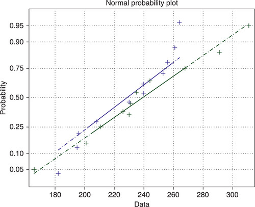
h = 0, it is unlikely that the samples have different mean lifetimes.
The points in both samples follow approximately straight, solid lines (the first and third quartiles of the samples); this shows that the data are close to the normal distributions.
6.6.3 Testing a proportion
Comparing a population and sample sizes/proportions is one of the most common problems in statistical quality control.
Problem: Suppose we want to sample enough people in order to distinguish 30% of 33% of the votes for a candidate. The vote numbers are integer and discrete; thus, we should use a discrete distribution, for example a binomial distribution. Say the power of 80% is enough to enable us to be sure that we can reduce the second error type. To define sample size, use the sampsizepwr function with the 'p' test type parameter (binomial distribution) and the right-tailed test specification - because we are interested only in alternative values greater than 30%.
To solve this problem use the following commands:
> > p0 = 0.30;
> > p1 = 0.33;
> > power = 0.8;
> > N = sampsizepwr('p',p0,p1,power,[],'tail','right')
Warning: Values N > 200 are approximate. Plotting the power as a function of N may reveal lower N values that have the required power.
> In sampsizepwr at 135
N =
1500
The empty square brackets replace the omitted parameter n, sample size, which is the output parameter of the used sampsizepwr form. A warning message informs us that the answer is an approximate calculation. If we look at the power function for different sample sizes, we can see that in general, the function is increasing, but is irregular because the binomial distribution is discrete. A more precise value is N = 1478 and can be defined by carrying out a more detailed analysis, which requires a greater level of knowledge in statistics and in MATLAB®, which is beyond the goals of this book. Additional information can be obtained by entering the samplesizedemo in the Command Window.
6.7 Questions for self-checking
1. If a null-hypothesis is rejected, which value is assigned by a test command to the h variable? (a) 0, (b) 1, (c) NaN.
2. Which parameter of the [h,p] = ttest(x,m,alpha) command contains the test decision? (a) input parameter m, (b) input parameter alpha, (c) output parameter p, (d) output parameter h.
3. If a t-test on a pair of samples shows h = 0, we can conclude that (a) there is no significant difference between the samples, (b) there is a significant difference between the samples, (c) the test fails to reject the null hypothesis?
4. The command for the Wilcoxon signed rank test is: (a) signrank, (b) ranksum, (c) sampsizepwr, (d) lillietest?
5. The command written as [h,p] = ttest(x,m) performs (a) a paired t-test, (b) a t-test on the assumption that the data in x come from a distribution with the m mean, (c) a two-sample test?
6. The kstest2 command performs (a) a two-sample Kolmogorov- Smirnov goodness-of-fit hypothesis test, (b) a single sample Kolmogorov-Smirnov goodness-of-fit test, (c) Lilliefors' composite goodness-of-fit test?
7. For a t-test the [h,p] = ttest(x,y) command was used; which value of the significance level is accepted in the test? (a) 1%, (b) 5%, (c) 3%.
8. If we have two unequal samples of data, which of the following commands should be used to define that their mean is different? (a) ttest2, (b) ttest, (c) kstest.
6.8 Answers to selected questions
4. (a) signrank.
6. (a) two-sample Kolmogorov-Smirnov goodness-of-fit hypothesis test.
8. (a) ttest2.