
CHAPTER 5
The Strategic Role of Information in Sales Management
LEARNING OBJECTIVES
Sales managers are both users and generators of information. The sales manager’s role with regard to generating, analyzing, and disseminating information is vital to the success of both the firm’s marketing strategy and the success of its individual salespeople. Important decisions at all levels of the organization are affected by how well sales managers use information.
This chapter presents a look at several of the key ways sales managers perform this vital information management role including forecasting sales, setting quotas, establishing the size and territory design of the sales force, and performing sales analysis for managerial decision making. Specifically, after reading this chapter, you should be able to:
- Discuss the differences between market potential, sales potential, sales forecast, and sales quota.
- Understand the various methods by which sales managers develop sales forecasts.
- Outline the process of setting a sales quota.
- Explain the various types of quotas used in sales management.
- Discuss key approaches to determining sales force size.
- Describe the sales territory design process.
- Understand the importance of sales analysis for managerial decision making.
- Conduct a sales analysis.
USING INFORMATION IN MANAGERIAL DECISION MAKING AND PLANNING
It has been said that information is the fuel that drives the engine in managerial decision making. This is no different in sales management. Sales managers are charged with making decisions and developing plans that impact multifaceted areas of a company. One of these areas, sales forecasting, is directly linked with the overall market opportunity analysis of the firm.
Developing sales forecasts is one of the most important uses of information by sales managers. And concurrently, the sales forecasts they develop become an integral part of an organization’s overall planning and strategy development efforts. Without good sales forecasts, it is impossible for companies to properly invest against their market opportunities. Sales managers must understand the various approaches to forecasting and appreciate the value of utilizing multiple methods of sales forecasting before making a decision on the final forecast to present to the firm.
For the sales manager, the forecast allows for the development of estimates of demand for individual sales territories and subsequently for the establishment of specific sales quotas by territory and by salesperson. Quotas are very important both to the firm and to its individual salespeople. For the firm, the aggregate of sales quotas during a particular performance period represents an operationalization of the sales forecast, and thus progress by the sales organization toward quota achievement is closely monitored by top management. For the individual salesperson, quotas provide specific goals to work toward that are tailored to his or her sales territory. Ordinarily, important elements of compensation and other rewards are linked to quota achievement. Because of the importance of quotas, sales managers must make certain they use the information available to select the proper type of quotas for the situation and to ensure that the level of the quotas is established in a fair and accurate manner.
Another important use of information by sales managers is in determining the optimal size of the sales force. A variety of quantitative analytical approaches are available for making this determination, all of which are driven by information. Once the size of the sales force is set, sales managers turn their analysis toward designing the sales territories. Finally, information is vital to the capability of sales managers to perform sales analyses.
In this chapter, we discuss each of these major strategic uses of information by sales managers and provide a context for sales managers to make better use of the information available to them for decision making.
INTRODUCTION TO MARKET OPPORTUNITY ANALYSIS
Market opportunity analysis requires an understanding of the differences in the notions of market potential, sales potential, sales forecast, and sales quota.
Market potential is an estimate of the possible sales of a commodity, a group of commodities, or a service for an entire industry in a market during a stated period under ideal conditions. A market is a customer group in a specific geographic area.
Sales potential refers to the portion of the market potential that a particular firm can reasonably expect to achieve. Market potential represents the maximum possible sales for all sellers of the good or service under ideal conditions, while sales potential reflects the maximum possible sales for an individual firm.
The sales forecast is an estimate of the dollar or unit sales for a specified future period. The forecast may be for a specified item of merchandise or for an entire line. It may be for a market as a whole or for any portion of it. Importantly, a sales forecast specifies the commodity, customer group, geographic area, and time period and includes a specific marketing plan and accompanying marketing program as essential elements. If the proposed plan is changed, predicted sales are also expected to change.
Naturally, forecast sales are typically less than the company’s sales potential for a number of reasons. The firm may not have sufficient production capacity to realize its full potential, or its distribution network may not be sufficiently developed, or its financial resources may be limited. Likewise, forecast sales for an industry are typically less than the industry’s market potential.
Sales quotas are sales goals assigned to a marketing unit for use in managing sales efforts. The marketing unit in question might be an individual salesperson, a sales territory, a branch office, a region, a dealer or distributor, or a district, just to name a few possibilities. Each salesperson in each sales territory might be assigned a sales volume goal for the next year. Sales quotas are typically a key measurement used to evaluate the personal selling effort. They apply to specific periods and can be specified in great detail—for example, sales of a particular item to a specified customer by sales rep J. Jones in June.
Exhibit 5.1 shows the relationship between potentials, forecasts, and quotas. Typically the process begins with an assessment of the economic environment. Sometimes this is simply an implicit assessment of the immediate future. Then, given an initial estimate of industry potential and the company’s competitive position, the firm’s sales potential can be estimated. This in turn leads to an initial sales forecast, often based on the presumption that the marketing effort will be similar to what it was last year. The initial forecast is then compared with objectives established for the proposed marketing effort. If the marketing program is expected to achieve the objectives, both the program and the sales forecast are adopted. That is rare, however. Usually it is necessary to redesign the marketing program and then revise the sales forecast, often several times.
EXHIBIT 5.1
Market potential, sales potential, and sales forecasting process

The objectives may also need revising, but eventually the process should produce agreement between the forecast or expected sales and the objectives. The sales forecast is then used as a key input in setting individual sales quotas (goals). In addition, it also serves as a basic piece of information in establishing budgets for the various functional areas.
METHODS OF SALES FORECASTING
The sales forecast is one of the most important information tools used by management and lies at the heart of most companies’ planning efforts. Top management uses the sales forecast to allocate resources among functional areas and to control the operations of the firm. Finance uses it to project cash flows, to decide on capital appropriations, and to establish operating budgets. Production uses it to determine quantities and schedules and to control inventories. Human resources uses it to plan personnel requirements and also as an input in collective bargaining. Purchasing uses it to plan the company’s overall materials requirements and also to schedule their arrival. Marketing uses it to plan marketing and sales programs and to allocate resources among the various marketing activities. The importance of accurate sales forecasts is exacerbated as companies coordinate their efforts on a global scale.
The sales forecast is also of fundamental importance in planning and evaluating the personal selling effort. Sales managers use it for setting sales quotas, as input to the compensation plan, and in evaluating the field sales force, among other things. Because sales managers rely so heavily on sales forecasts for decision making, and also are integral to the formulation of sales forecasts, it is important that they be familiar with the techniques used in forecast development. The subjective and objective methods discussed in this chapter are listed in Exhibit 5.2.1
EXHIBIT 5.2
Classification of sales forecasting methods

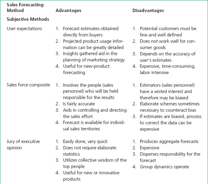
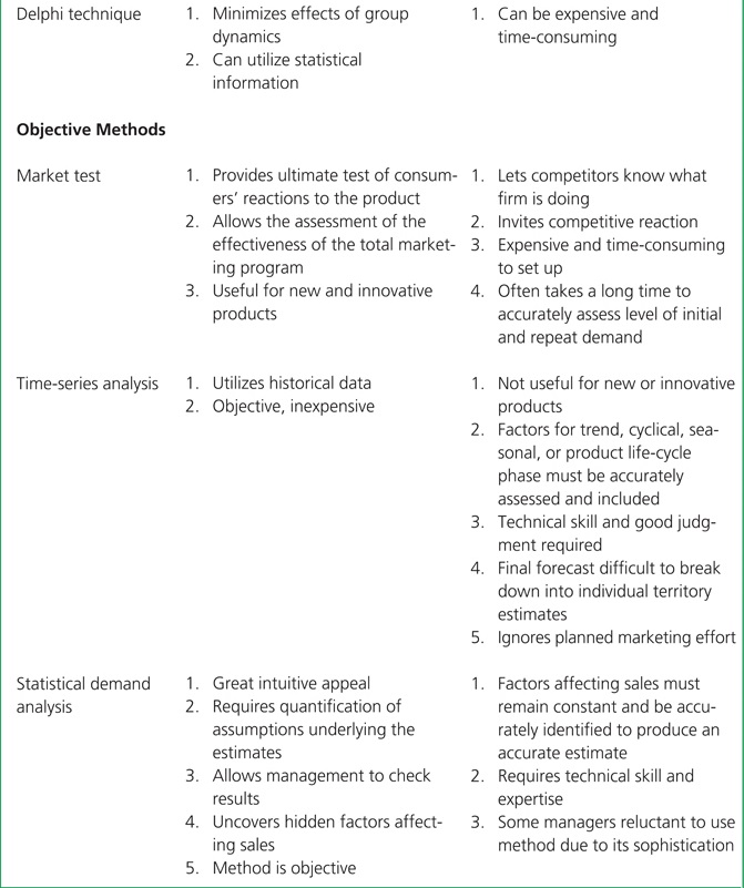
Each method has advantages and disadvantages, which are summarized in Exhibit 5.3, and the decision of which method to use will not always be clear.2 In a typical company, the decision will likely depend on its level of technical sophistication, the existence of historic sales data, and the proposed use of the forecast.
EXHIBIT 5.3
Summary of advantages and disadvantages of various sales forecasting techniques
Subjective Methods of Forecasting
Subjective forecasting methods do not rely primarily on sophisticated quantitative (empirical) analytical approaches in developing the forecast.
User Expectations
The user expectations method of forecasting sales is also known as the buyers’ intentions method because it relies on answers from customers regarding their expected consumption or purchases of the product.
The user expectations method of forecasting sales may provide estimates closer to market or sales potential than to sales forecasts. In reality, user groups would have difficulty anticipating the industry’s or a particular firm’s marketing efforts. Rather, the user estimates reflect their anticipated needs. From the sellers’ standpoint, they provide a measure of the opportunities available among a particular segment of users.
Sales Force Composite
The sales force composite method of forecasting sales is so named because the initial input is the opinion of each member of the field sales staff. Each person states how much he or she expects to sell during the forecast period. Subsequently, these estimates are typically adjusted at various levels of sales management. They are likely to be checked, discussed, and possibly changed by the branch manager and on up the sales organization chart until the figures are finally accepted at corporate headquarters.
When forecasting via sales force composite, organizations typically use historical information about the accuracy of the salespeople’s estimates to make adjust-ments to the raw forecast data provided by the field sales organization. For various reasons, salespeople may be motivated to either underestimate or overestimate what they expect to sell during a period. For example, if quotas are derived from the forecast, salespeople may underestimate their sales volume in order to “sandbag” business and get assigned a smaller quota. Thus, when their sales results come in they give the appearance of a stronger performance. Alternatively, if certain of the company’s products are in short supply (such as in a materials shortage or rapid growth market) or are available to customers in limited quantities (such as a short-term promotion), salespeople may overestimate their sales volume in hopes of securing a greater allocation of scarce products.
Jury of Executive Opinion
The jury of executive opinion (or jury of expert opinion) method is a formal or informal internal poll of key executives within the selling company in order to gain their assessment of sales possibilities. The separate assessments are combined into a sales forecast for the company. Sometimes this is done by simply averaging the individual judgments; but other times disparate views are resolved through group discussion toward consensus. The initial views may reflect no more than the executive’s hunch about what is going to happen, or the opinion may be based on considerable factual material, sometimes even an initial forecast prepared by other means.
Delphi Technique
In gaining expert opinion, one method for controlling group dynamics to produce a more accurate forecast is the Delphi technique. Delphi uses an iterative approach with repeated measurement and controlled anonymous feedback, instead of direct confrontation and debate among the experts preparing the forecast.3 Each individual involved prepares a forecast using whatever facts, figures, and general knowledge of the environment he or she has available. Then the forecasts are collected, and an anonymous summary is prepared by the person supervising the process. The summary is distributed to each person who participated in the initial phase. Typically, the summary lists each forecast figure, the average (median), and some summary measure of the spread of the estimates. Often, those whose initial estimates fell outside the midrange of responses are asked to express their reasons for these extreme positions. These explanations are then incorporated into the summary. The participants study the summary and submit a revised forecast. The process is then repeated. Typically, several rounds of these iterations take place. The method is based on the premise that, with repeated measurements (1) the range of responses will decrease and the estimates will converge; and (2) the total group response or median will move successively toward the “correct” or “true” answer.
Objective Methods of Forecasting
Objective forecasting methods rely primarily on more sophisticated quantitative (empirical) analytical approaches in developing the forecast.
Market Test
The typical market test (or test market) involves placing a product in several representative geographic areas to see how well it performs and then projecting that experience to the market as a whole. Often this is done for a new product or an improved version of an old product.
Many firms consider the market test to be the final gauge of consumer acceptance of a new product and ultimate measure of market potential. A. C. Nielsen data, for example, indicate roughly three out of four products that have been test marketed succeed, whereas four out of five that have not been test marketed fail. Despite this fact, market tests have several drawbacks:
- Market tests are costly to administer and are more conducive to testing of consumer products than industrial products.
- The time involved in conducting a market test can be considerable.
- Because a product is being test marketed, it receives more attention in the market test than it can ever receive on a broader/full market scale, giving an unrealistic picture of the product’s potential.
- A market test, because it is so visible to competitors, can reveal a firm’s hand on its new-product launch strategy, thus allowing competitors time to formulate a market response before full market introduction.
All in all, a market test can be a highly successful sales forecasting technique but one that should not be used unless and until all the positives and negatives have been evaluated by management.
Time-Series Analysis
Approaches to sales forecasting using time-series analysis rely on the analysis of historical data to develop a prediction for the future. The sophistication of these analyses can vary widely. At the most simplistic extreme, the forecaster might simply forecast next year’s sales to be equal to this year’s sales. Such a forecast might be reasonably accurate for a mature industry that is experiencing little growth or market turbulence. However, barring these conditions, more sophisticated time-series approaches must be considered. Three of these methods, moving averages, exponential smoothing, and decomposition, are discussed here.4
Moving Average
The moving average method is conceptually quite simple. Consider the forecast that next year’s sales will be equal to this year’s sales. Such a forecast might be subject to large error if there is much fluctuation in sales from one year to the next. To allow for such randomness, we might consider using some kind of average of recent values. For example, we might average the last two years’ sales, the last three years’ sales, the last five years’ sales, or any number of other periods. The forecast would simply be the average that resulted. The number of observations included in the average is typically determined by trial and error. Differing numbers of periods are tried, and the number of periods that produces the most accurate forecasts of the trial data is used to develop the forecast model. Once determined, it remains constant. The term moving average is used because a new average is computed and used as a forecast as each new observation becomes available.
Exhibit 5.4 presents a moving average forecast example with 16 years of historical sales data and also the resulting forecasts for a number of years using two- and four-year moving averages. Exhibit 5.5 displays the results graphically. The entry 4,305 for 2007, under the two-year moving average method, for example, is the average of the sales of 4,200 units in 2005 and 4,410 units in 2006. Similarly, the forecast of 5,520 units in 2020 represents the average of the number of units sold in 2018 and 2019. The forecast of 5,772 units in 2020 under the four-year moving average method, on the other hand, represents the average number of units sold during the four-year period 2016–2020. Obviously, it takes more data to begin forecasting with four-year than with two-year moving averages. This is an important consideration when starting to forecast sales for a new product.
EXHIBIT 5.4
Example of a moving average forecast

EXHIBIT 5.5
Graph of actual and forecast sales using moving averages

Exponential Smoothing
The method of moving averages gives equal weight to each of the last n values in forecasting the next value, where n represents the number of years used. Thus, when n = 4 (the four-year moving average is being used), equal weight is given to each of the last four years’ sales in predicting the sales for next year. In a four-year moving average, no weight is given to any sales five or more years previous.
Exponential smoothing is a type of moving average. However, instead of weighting all observations equally in generating the forecast, exponential smoothing weights the most recent observations heaviest, for good reason. The most recent observations contain the most information about what is likely to happen in the future, and they should logically be given more weight. Exponential smoothing yields more accurate quotas than traditional and relative-growth methods for setting quotas and is able to detect patterns in historical geographic sales data. Higher quota accuracy leads to more accurate territory sizing and market potential, as well as improved motivation.
The key decision affecting the use of exponential smoothing is the choice of the smoothing constant, referred to as α in the algorithm for calculating exponential smoothing, which is constrained to be between 0 and 1. High values of α give great weight to recent observations and little weight to distant sales; low values of α, on the other hand, give more weight to older observations. If sales change slowly, low values of α work fine. When sales experience rapid changes and fluctuations, however, high values of α should be used so that the forecast series responds to these changes quickly. The value of α is normally determined empirically; various values of α are tried, and the one that produces the smallest forecast error when applied to the historical series is adopted.
Decomposition
The decomposition method of sales forecasting is typically applied to monthly or quarterly data where a seasonal pattern is evident and the manager wishes to forecast sales not only for the year but also for each period in the year. It is important to determine what portion of sales changes represents an overall, fundamental change in demand and what portion is due to seasonality in demand. For example, Banana Boat would like to separate out how much of its sales increase in suntan lotion is attributable to the general trend toward increased skin protection from the sun and how much is due to peak seasonal demand in May–September. The decomposition method attempts to isolate four separate portions of a time series: the trend, cyclical, seasonal, and random factors.
- The trend reflects the long-run changes experienced in the series when the cyclical, seasonal, and irregular components are removed. It is typically assumed to be a straight line.
- The cyclical factor is not always present because it reflects the waves in a series when the seasonal and irregular components are removed. These ups and downs typically occur over a long period, perhaps two to five years. Some products experience little cyclical fluctuation (canned peas), whereas others experience a great deal (housing starts).
- Seasonality reflects the annual fluctuation in the series due to the natural seasons. The seasonal factor normally repeats itself each year, although the exact pattern of sales may be different from year to year.
- The random factor is what is left after the influence of the trend, cyclical, and seasonal factors is removed.
Exhibit 5.6 shows the calculation of a simple seasonal index based on five years of sales history. The data suggests definite seasonal and trend components in the series. The fourth quarter of every year is always the best quarter; the first quarter is the worst. At the same time, sales each year are higher than they were the year previous. One could calculate a seasonal index for each year by simply dividing quarterly sales by the yearly average per quarter. It is much more typical, though, to base the calculation of the seasonal index on several years of data to smooth out the random fluctuations that occur by quarter.
EXHIBIT 5.6
Calculation of a seasonal index

In using the decomposition method, the analyst typically first determines the seasonal pattern and removes its impact to identify the trend. Then the cyclical factor is estimated. After the three components are isolated, the forecast is developed by applying each factor in turn to the historical data.
Statistical Demand Analysis
Time-series methods attempt to determine the relationship between sales and time as the basis of the forecast for the future. Statistical demand analysis attempts to determine the relationship between sales and the important factors affecting sales to forecast the future. Typically, regression analysis is used to estimate the relationship. The emphasis is not to isolate all factors that affect sales but simply to identify those that have the most dramatic impact on sales and then to estimate the magnitude of the impact. The predictor variables in statistical demand analysis often are historical indexes such as leading economic indicators and other similar measures. For example, a lumber products company might use housing starts, interest rates, and a seasonal shift in demand during summer months to forecast its sales.
CHOOSING A FORECASTING METHOD
The sales manager faced with a forecasting problem has a dilemma: Which forecasting method should be used and how accurate is the forecast likely to be? The dilemma is particularly acute when several methods are tried and the forecasts don’t agree, which is more often the norm rather than the exception.
A number of studies have attempted to assess forecast accuracy using the various techniques. Some studies have been conducted within individual companies; others have used selected data series to which the various forecasting techniques have been systematically applied. One of the most extensive comparisons involved 1,001 time series from a variety of sources in which each series was forecast with each of 24 extrapolation methods. The general conclusion was that the method used made little difference with respect to forecast accuracy.5 Similarly, comparisons of forecast accuracy of objective versus subjective methods gave no clear conclusion as to which method is superior. Some of the comparisons seem to favor the quantitative methods,6 but others found that the subjective methods produce more accurate forecasts.7
In general, the various forecast comparisons suggest that no method is likely to be superior under all conditions. Rather, a number of factors are likely to affect the superiority of any particular technique, including the stability of the data series, the time horizon, the degree of structure imposed on the process, the degree to which computers were used, and deseasonalization of the data. Overall, the best approach seems to be the utilization of multiple methods of forecasting, including a combination of subjective and objective methods, comparing the results, and then employing managerial judgment to make a decision on the final forecast.
Increasingly, firms are turning to scenario planning when developing sales forecasts. Scenario planning involves asking those preparing the forecast a series of “what-if” questions, where the what-ifs reflect different environmental changes that could occur. Some very unlikely changes are considered along with more probable events. The key idea is not so much to have one scenario that gets it right but rather to have a set of scenarios that illuminate the major forces driving the system, their interrelationships, and the critical uncertainties.8
DEVELOPING TERRITORY ESTIMATES
Not only must firms develop global estimates of demand, but most also develop territory-by-territory estimates. Territory estimates recognize the condition that the potential for any product may not be uniform by area. Territory demand estimates allow for effective planning, directing, and controlling of salespeople in that the estimates affect the following:
- The design of sales territories.
- The procedures used to identify potential customers.
- The establishment of sales quotas.
- Compensation levels and the mix of components in the firm’s sales compensation scheme.
- The evaluation of salespeople’s performance.
The development of territory demand estimates is typically different for industrial versus consumer goods. Territory demand estimates for industrial goods are often developed by relating sales to some common denominator. The common denominator or market factor might be the number of total employees, number of production employees, value added by manufacturing process, value of materials consumed, value of products shipped, or expenditures for new plant and equipment. Say the ratio of sales per employee is developed for each of several identifiable markets. By then looking at the number of employees in a particular geographic area within each of those identifiable markets, one can estimate the total demand for the product within the area.
The identifiable markets are usually defined using the North American Industry Classification System (NAICS). The NAICS replaced the former system of Standard Industrial Classification (SIC) codes. These systems were developed by the U.S. Bureau of the Census for organizing the reporting of business information such as employment, value added in manufacturing, capital expenditures, and total sales. Each major industry in the United States is assigned a two-digit number, indicating the group to which it belongs. The types of businesses making up each industry are further identified by additional digits.
While firms selling to industrial consumers rely most heavily on identifiable market segments using NAICS codes when estimating territory demand, sellers of consumer goods are more apt to rely on aggregate conditions in each territory. Sometimes this will be a single variable or market factor like the number of households, population, or perhaps the level of income in the area. In other instances, the firm attempts to relate demand to several variables combined in a systematic way. The demand for washing machines, for example, has been shown through statistical demand regression analysis to be a function of the following predictor variables: (1) the level of consumers’ stock of washing machines, (2) the number of wired dwelling units, (3) disposable personal income, (4) net credit, and (5) the price index for house furnishings. Since these statistics are published by area, a firm can use the regression equation to estimate demand by area.
Many firms are willing to expend the effort necessary to develop an expression for the relationship between total demand for the product and several variables that are logically related to its sales. Many other firms, however, are content to base their estimates of territory demand on one of the standard multiple-factor indexes that have been developed. A buying power index (BPI) is an index composed of weighted measures of disposable income, sales data, and market factors for a specific region. Such an index is used by sales organizations to determine the revenue potential for a particular region. If the index does not correlate well with sales of the product, then the firm is probably better off (1) using a single market factor or (2) developing its own index using factors logically related to sales and some a priori or empirically determined weights regarding their relative importance.9
PURPOSES AND CHARACTERISTICS OF SALES QUOTAS
As discussed earlier in the chapter, goals assigned to salespeople are called quotas. Quotas are one of the most valuable devices sales managers have for planning the field selling effort, and they are indispensable for evaluating the effectiveness of that effort. They help managers plan the amount of sales and profit that will be available at the end of the planning period and anticipate the activities of the sales team. Quotas are also often used to motivate salespeople and as such must be reasonable. Volume quotas are typically set to a level that is less than the sales potential in the territory and equal to or slightly above the sales forecast for the territory, although they also may be set less than the sales forecast if conditions warrant.
Sales quotas apply to specific periods and may be expressed in dollars or physical units. Thus, management can specify quarterly, annual, and longer-term quotas for each of the company’s field representatives in both dollars and physical units. It might even specify these goals for individual products and customers. The product quotas can be varied systematically to reflect the profitability of different items in the line, and customer quotas can be varied to reflect the relative desirability of serving particular accounts.
Purposes of Quotas
Quotas facilitate the planning and control of the field selling effort in a number of ways. Two important contributions of sales quotas are in (1) providing incentives for sales representatives and (2) evaluating salespeople’s performance.
Quotas serve as incentives for sales in several ways. In essence, they are an objective to be secured and a challenge to be met. For example, the definite objective of selling $200,000 worth of product X this year, particularly with the opportunity to achieve some desired reward if the quota is met or exceeded, is more motivation to most salespeople than the indefinite charge to go out and do better. It seems one can always do better. Quotas also influence salespeople’s incentive through sales contests. A key notion underlying such contests is that those who perform “best” will receive the contest prizes. Quotas can also create incentive via their key role in the compensation systems of most firms. More will be said about these reward and compensation issues in later chapters, but it should be noted here that many firms use a commission or bonus plan, sometimes in conjunction with their base salary plan. In such schemes, salespeople are paid in direct proportion to what they sell (commission plan), or they receive some percentage increment for sales in excess of target sales (bonus plan). Typically, such plans are tied directly to sales quotas. Even when salespeople are compensated with salary only, quotas can provide incentive when salary raises are tied to quota attainment in the previous year. The Leadership box makes a strong case for the importance of strong linkages between sales process and attainment of quota by salespeople.
Quotas also provide a quantitative (objective) standard against which the performance of individual sales representatives or other marketing units can be evaluated. They allow management to recognize salespeople who are performing particularly well and those who may be experiencing difficulty in performance. They provide a basis for developmental actions by the manager and salesperson to ensure a greater level of performance in the future. Issues of performance evaluation of salespeople are discussed in detail in Chapter 13.
Characteristics of a Good Quota
For a quota to be effective, it must be (1) attainable, (2) easy to understand, (3) complete, and (4) timely. Some argue that quotas should be set high so they can be achieved only with extraordinary effort. Although most salespeople may not reach their quotas, the argument is that they are spurred to greater effort than they would have expended in the absence of such a “carrot.” Although perhaps intuitively appealing, high quotas can cause problems. They can create ill will among salespeople. They can also cause salespeople to engage in unethical and other undesirable behaviors to make their quotas.10 The use of very high “carrot” quotas seems to be the exception rather than the rule and is generally not recommended. The prevailing philosophy is that quotas should be realistic. They should represent attainable goals that can be achieved with normal or reasonable, not Herculean, efforts. That seems to motivate most salespeople best.
Quotas should be not only realistic but also easy to understand. Complex quota plans may cause suspicion and mistrust among sales representatives and thereby discourage rather than motivate them. It helps when salespeople can be shown exactly how their quotas were derived. They are much more likely to accept quotas that are related to market potential when they can see the assumptions used in translating the potential estimate into sales goals.
Another desirable feature of a quota plan is that it is complete. It should cover the many criteria on which sales reps are to be judged. Thus, if all sales representatives are supposed to engage in new-account development, it is important to specify how much. Otherwise that activity will likely be neglected while the salesperson pursues volume and profit goals. Similarly, volume and profit goals should be adjusted to allow for the time the representative has to spend identifying and soliciting new accounts.
Finally, the quota system should allow for timely feedback of results to salespeople. Quotas for a sales period should be calculated and announced right away. Delays in providing this information not only dilute the advantages of using quotas but also create ambiguity, as the salesperson gets well into another performance period without knowing how he or she fared in the prior period.
SETTING QUOTAS
In setting quotas, the sales manager must first decide on the types of quotas the firm will use. Then, specific quota levels must be established. The calculation of quotas has changed due to the advances of technology. Factors such as big data, data mining, and the rise of the Internet and social media have allowed organizations to more accurately calculate quotas with current and valuable information.
Types of Quotas
There are three basic types of quotas: (1) those emphasizing sales or some aspect of sales volume, (2) those that focus on the activities in which sales representatives are supposed to engage, and (3) those that examine financial criteria such as gross margin or contribution to overhead. Sales volume quotas are the most popular.11
Sales Volume Quotas
The popularity of sales volume quotas, those that emphasize dollar sales or some other aspect of sales volume, is understandable. They can be related directly to market potential and thereby be made more credible, are easily understood by the salespeople who must achieve them, and are consistent with what most salespeople envision their jobs to be—that is, to sell. Sales volume quotas may be expressed in dollars, physical units, or points.
The concept of point quotas deserves explanation. A certain number of points are given for each dollar or unit sale of particular products. For example, each $100 of sales of product X might be worth three points; of product Y, two points; and of product Z, one point. Alternatively, each ton of steel tubing sold might be worth five points, while each ton of bar stock might be worth only two points. The total sales quota for the salesperson is expressed as the total number of points he or she is expected to achieve. The point system is typically used when a firm wants to emphasize certain products in the line. Those that are more profitable, for example, might be assigned more points.
Point quotas can also be used to promote selective emphases. New products might receive more points than old ones to encourage sales representatives to push them. A given dollar of sales to new accounts might be worth more points than the same level of sales to more established accounts. Point quota systems allow sales managers to design quota systems that promote certain desired goals, and at the same time point quotas can be easily understood by salespeople.
Activity Quotas
Activity quotas attempt to recognize the investment nature of a salesperson’s efforts. For example, the letter to a prospect, the product demonstration, and the arrangement of a display may not produce an immediate sale. On the other hand, they may influence a future sale. If the quota system emphasizes only sales volume, salespeople may be inclined to neglect these activities. Today, many activities are necessary to support long-term client relationships. It is appropriate that these activities be considered for quota development. Some common types of activity quotas are listed in Exhibit 5.7.
EXHIBIT 5.7
Common types of activity quotas

Financial Quotas
Financial quotas help focus salespeople on the cost and profit implications of what they sell. All else being equal, it is easy to understand that salespeople might emphasize products in their line that are relatively easy to sell or concentrate on customers with whom they feel most comfortable interacting. Unfortunately, these products may be costly to produce and have a lower-than-average return, and these customers may not purchase much and may be less profitable than other potential accounts. Financial quotas attempt to direct salespeople’s efforts to more profitable products and customers. Common bases for developing financial quotas are gross margin, net profit, and selling expenses, although most any financial measure could be used.
Administering financial quotas can present difficulties. Their calculation is not straightforward. And the profit a salesperson produces is affected by many factors beyond his or her control—competitive reaction, economic conditions, and the firm’s willingness to negotiate on price, for example. Many would argue that in most cases it is unreasonable to hold an individual salesperson responsible for such external influences.
Quota Level
Next, the sales manager must decide the level for each type of quota. In establishing these levels, the sales manager must balance a number of factors, including the potential available in the territory, the impact of the quota level on the salesperson’s motivation, the long-term objectives of the company, and the impact on short-term profitability. When discussing quota levels, it is useful to separate sales volume, activity, and financial quotas.
Sales Volume Quotas
Some firms simply set sales volume quotas on the basis of past sales. Each marketing unit is exhorted to “beat last year’s sales.” Sometimes the standard is the average of sales in the territory over some past time period—five years, for example. The most attractive feature of this quota-setting scheme is that it is easy to administer. One does not have to engage in an extensive analysis to determine what the quotas should be. This makes it inexpensive to use. Also, salespeople readily understand it.
Unfortunately, such quotas ignore current conditions. A territory may be rapidly growing, and the influx of new potential customers could justify a much larger increase than the 7 percent established by the overall company’s sales forecast. Alternatively, the territory might be so intensely competitive or the business climate may be so poor that any increase in the assigned sales quota is not justified.
A quota based solely on past sales ignores territory potentials and provides a poor yardstick for evaluating individual sales reps. Two salespeople, for example, might each have generated $300,000 in sales last year. It clearly makes a difference in what one can expect from each of them this year if the market potential in one territory is $500,000 while that in the other is $1 million. The firm may be forgoing tremendous market opportunities simply because it is unaware of them.
A quota based solely on past years’ sales can also demoralize salespeople and cause undesirable behaviors. For example, a salesperson who has realized quota for one year may be tempted to delay placing orders secured at the end of the year until the new accounting cycle begins. This accomplishes two things: It makes his or her quota for the next year lower, and it gives him or her a start on satisfying that quota.
Territory potential provides a useful start for establishing quotas for territory sales volume. However, the firm should not adhere strictly to a formula that relates quota to potential, but it should attempt to reflect the special situations within each territory.
Determining how to set territory quotas that reflect the special situations within each territory is often difficult. On one hand, the sales representative who serves the territory should be involved in setting the territory quota, because he or she should have the most intimate knowledge of the conditions in the territory. On the other hand, since the rep will be affected by the quota established, he or she may not be impartial. One might expect sales representatives to understate potential to generate lower, easier-to-reach quotas.
Activity Quotas
The levels for activity quotas are most likely to be set according to the territory conditions. They require a detailed analysis of the work needed to cover the territory effectively. Activity quotas are affected by the size of the territory and by the number of accounts and prospects the salesperson is expected to call on. The size of the representative’s customers can also make a difference, as can their purchasing patterns. These factors affect the number of times the salesperson needs to call on them in the period, the number of service calls or calls to demonstrate the use of the firm’s equipment he or she must make, and so on.
The inputs for activity quotas can come from at least three sources: (1) discussions between the sales representative serving the territory and the sales manager, (2) the salesperson’s reports, and (3) research on the market and its potential.
Financial Quotas
The levels of financial quotas are typically set to reflect the financial goals of the firm. For example, a firm may want a particular net profit or gross margin on all sales in a territory. Suppose the potential for a representative is basically concentrated on two products—one with a gross margin of 30 percent and one with a gross margin of 40 percent. The sales manager could shift the relative attention given to one versus the other by assigning a gross margin goal of 37 percent. The salesperson would then have to sell a greater proportion of the products with 40 percent margin to achieve that goal than if the goal were 34 percent.
DETERMINING SALES FORCE SIZE
Another critical use of information by sales managers is in determining the size of the sales force. Salespeople are among the most productive assets of a company, and they are also among the most expensive. Determining the optimal number to employ presents several fundamental dilemmas. On the one hand, increasing the number of salespeople will increase sales volume. On the other hand, it will also increase costs. Achieving the optimal balance between these considerations, although difficult, is vitally important to a firm’s success.
The optimal number of territories depends on the design of the individual territories. Different assignments to salespeople and even different call patterns can produce different sales levels. Of course, the number of calls the sales force must make directly affects the number of salespeople the firm needs. In sum, the number of sales territories and the design of individual territories must be looked at as interrelated decisions whose outcomes affect each other.
The decisions need to be made jointly and not sequentially. Sales force deployment refers to the three interrelated decisions of (1) sales force size or the number of territories, (2) design of the individual territories, and (3) allocation of the total selling effort to accounts. Such simultaneous decisions are implemented through software-driven sales force deployment models. At the same time, it is useful for discussion purposes to separate these issues so as to call attention to the underlying considerations of each. Consequently, the subsequent discussion first addresses the issue of sales force size and then the issue of sales territory design. However, the size of the sales force may need to be revised as a result of the sales territory design.12
Several techniques are available for determining the size of the field sales force. Three of the more popular are the (1) breakdown, (2) workload, and (3) incremental methods.
Breakdown Method
The breakdown method is conceptually one of the simplest. An average salesperson is treated as a salesperson unit, and each salesperson unit is assumed to possess the same productivity potential. To determine the size of the sales force needed, divide total forecast sales for the company by the sales likely to be produced by each individual. Mathematically,
Thus, a firm that had forecast sales of $5 million and in which each salesperson unit could be expected to sell $250,000 would need 20 salespeople. Although conceptually simple and easy to use, the breakdown method is not without its problems. For one thing, it uses reverse logic. It treats sales force size as a consequence of sales volume; instead, determining the number of salespeople needed should be a proactive element of the overall strategic marketing plan. Also, the estimate of productivity per salesperson can be problematic in that it fails to account for differences in (1) ability levels of salespeople, (2) potential in the markets they service, and (3) level of competition across sales territories. Then too, the breakdown method does not take into account turnover in the sales force. New salespeople are usually not as productive as those who have been on the job for several years. The formula can be modified to allow for sales force turnover, but it loses some of its simplicity and conceptual appeal.
Finally, a key shortcoming of the breakdown method is that it does not allow for profitability. It treats sales as the end in itself rather than as the means to an end. The number of salespeople is determined as a function of the level of forecast sales, not as a determinant of targeted profit.
Workload Method
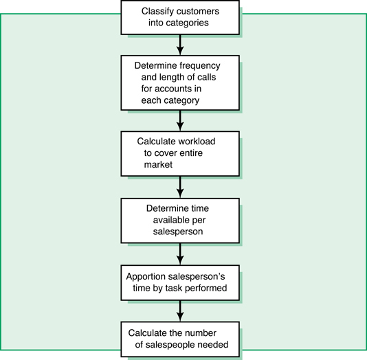
The basic premise underlying the workload method of determining sales force size (or, as it is sometimes called, the buildup method) is that all sales personnel should shoulder an equal amount of work. Management estimates the work required to serve the entire market. The total work calculation is treated as a function of the number of accounts, how often each should be called on, and for how long. This estimate is then divided by the amount of work an individual salesperson should be able to handle, and the result is the total number of salespeople required.13 Specifically, the method consists of six steps, as illustrated in Exhibit 5.8 and discussed next.
EXHIBIT 5.8
Steps to determine sales force size by the workload method
- Classify all the firm’s customers into categories. Often the classification is based on the level of sales to each customer. A popular approach is to identify and prioritize accounts as A, B, or C based on sales volume. Classification could be based on other criteria also, such as the customer’s type of business, credit rating, product line, and potential for future purchases.
Any classification system should reflect the different amounts of selling effort required to service the different classes of accounts and consequently the attractiveness of each class of accounts to the firm. Suppose, for example, the firm had 1,030 accounts that could be classified into three basic types or classes, as follows:
- Determine the frequency with which each type of account should be called upon and the desired length of each call. These inputs can be generated in several ways. They can be based directly on the judgments of management, or they might be based on more formal analysis of historical information. Suppose the firm estimates that class A accounts should be called on every two weeks, class B accounts once a month, and class C accounts every other month. It also estimates that the length of the typical call should be 60 minutes, 30 minutes, and 20 minutes, respectively. The number of contact hours per year for each type of account is thus calculated as
Class A: 26 times/year × 60 minutes/call = 1,560 minutes, or 26 hours
Class B: 12 times/year × 30 minutes/call = 360 minutes, or 6 hours
Class C: 6 times/year × 20 minutes/call = 120 minutes, or 2 hours
- Calculate the workload involved in covering the entire market. The total work involved in covering each class of account is given by multiplying the number of such accounts by the number of contact hours per year. These products are summed to estimate the work entailed in covering all the various types of accounts:
Class A: 200 accounts × 26 hours/account = 5,200 hours
Class B: 350 accounts × 6 hours/account = 2,100 hours
Class C: 480 accounts × 2 hours/account = 960 hours
Total = 8,260 hours
- Determine the time available per salesperson. For this calculation, one must estimate the number of hours the typical salesperson works per week and then multiply that by the number of weeks the representative will work during the year. Suppose the typical workweek is 40 hours and the average salesperson can be expected to work 48 weeks during the year, after allowing for vacation time, sickness, and other emergencies. This suggests the average representative has 1,920 hours available per year. That is,
40 hours/week × 48 weeks/year = 1,920 hours/year
- Apportion the salesperson’s time by task performed. Unfortunately, not all the salesperson’s time is consumed in face-to-face customer contact. Much of it is devoted to nonselling activities such as making reports, attending meetings, and making service calls. Another major portion may be spent traveling. Suppose a time study of salespeople’s effort suggested the following division:
Selling |
40 percent = |
768 hours/year |
Nonselling |
30 percent = |
576 hours/year |
Traveling |
30 percent = |
576 hours/year |
|
100 percent = |
1,920 hours/year |
- Calculate the number of salespeople needed. The number of salespeople the firm will need can now be readily determined by dividing the total number of hours needed to serve the entire market by the number of hours available per salesperson for selling. That is, by the calculation
The workload, or buildup, method is a very common way to determine sales force size. It has several attractive features. It is easy to understand, and it explicitly recognizes that different types of accounts should be called on with different frequencies. The inputs are readily available or can be secured without much trouble.
Unfortunately, it also possesses some weaknesses. It does not allow for differences in sales response among accounts that receive the same sales effort. Two class A accounts might respond differently to sales effort. One may be content with the products and services of the firm and continue to order even if the salesperson does not call every two weeks. Another, which does most of its business with a competitor, may willingly switch some of its orders if it receives more frequent contact. Also, the method does not explicitly consider the profitability of the call frequencies. It does not take into account such factors as the cost of servicing and the gross margins on the product mix purchased by the account.14
Finally, the method assumes that all salespeople use their time with equal efficiency—for example, that each will have 768 hours available for face-to-face selling. This is simply not true. Some are better able to plan their calls to generate more direct selling time. Those in smaller geographic territories can spend less time traveling and more time selling. Some more than others simply make good use of the selling time they have available, as the quality of time invested in a sales call is at least as important as the quantity of time spent. The buildup method does not explicitly consider these dimensions.
Incremental Method
The basic premise underlying the incremental method of determining sales force size is that sales representatives should be added as long as the incremental profit produced by their addition exceeds the incremental costs.15 The method recognizes that decreasing returns will likely be associated with the addition of salespeople. Thus, while one more salesperson might produce $300,000, two more might produce only $550,000 in new sales. The incremental sales produced by the first salesperson is $300,000 but for the second salesperson is $250,000. Suppose the addition of a third salesperson could be expected to produce $225,000 in new sales and a fourth, $200,000. Adding all four would increase sales by $975,000. Suppose further that the company’s profit margin was 20 percent, and placing another salesperson in the field cost $50,000 on average. This situation is summarized in Exhibit 5.9.
EXHIBIT 5.9
Illustration of the incremental approach to determining sales force size

The analysis in Exhibit 5.9 suggests that two salespeople should be added. At that point, the incremental profit from the additional salespeople equals the incremental cost. Adding more than two salespeople would cause profits to go down, as is seen by subtracting column (6) “total additional cost” from column (4) “total additional profit.”
The incremental approach to determining sales force size is conceptually sound. Also, it is consistent with the empirical evidence that decreasing returns can be expected with additional salespeople. Decreasing returns can also be expected with other territory design features such as the number of buyers per salesperson, the number of calls the salesperson makes on an account, and the actual time the representative spends in face-to-face contact.16
A key disadvantage of the incremental approach is that it is the most difficult to implement of the three approaches we have reviewed. Although the cost of an additional salesperson can be estimated with reasonable accuracy, estimating the likely profit is difficult. It depends on the additional revenue the salesperson is expected to produce, and that depends on how the territories are restructured, who is assigned to each territory, and how effective they might be. To compound things further, the profitability of the new arrangement also depends on the mix of products generating the sales increase and how profitable each is to the company.
DESIGNING SALES TERRITORIES
After the number of sales territories has been determined, the sales manager can address the issue of territory design. Warning: The examples in this section are U.S. focused—however, the concepts and process can be adapted to the needs and information availability of any geographic region of the globe. The stages involved in territory design are shown in Exhibit 5.10. The sales manager strives for the ideal of making all territories equal with respect to the amount of sales potential they contain and the amount of work it takes a salesperson to cover them effectively. When territories are basically equal in potential, it is easier to evaluate each representative’s performance and to compare salespeople. (A discussion of the potential problems in integrating territory difficulty differences into performance evaluations of salespeople is presented in Chapter 13.) Equal workloads tend to improve sales force morale and diminish disputes between management and the sales force. While considering these questions, the sales manager should take into account the impact on market response of particular territory structures and call frequencies. Obviously, it is difficult, if not impossible, to achieve an optimal balance with respect to all these factors. The sales manager should do his or her best to ensure the highest degree of fairness and equity in territory design.
EXHIBIT 5.10
Stages in territory design

Stages in Sales Territory Design
Step 1: Select Basic Control Unit
Some of the terminology in this section is heavily U.S.-centric for purposes of clear example, but those of you in other locales can easily translate the ideas into the context of your own countries. The basic control unit is the most elemental geographic area used to form sales territories—county or city, for example. As a general rule, small geographic control units are preferable to large ones. With large units, areas with low potential may be hidden by their inclusion in areas with high potential, and vice versa. This makes it difficult to pinpoint true geographic potential, which is a primary reason for forming geographically defined sales territories in the first place. Also, small control units make it easier to adjust sales territories when conditions warrant. It is much easier to reassign the accounts in a particular county from one salesperson to another, for example, than it is to reassign all the accounts in a state. Some commonly used basic control units are states, trading areas, counties, cities or metropolitan statistical areas (MSAs), and ZIP code areas.
States
Although it has become less popular, some companies still use states as a basic control because of inherent advantages. State boundaries are clearly defined and thus are simple and inexpensive to use. A good deal of statistical data are accumulated by state, which makes it easy to analyze territory potential.
One primary weakness of using states as control units is that buying habits, or consumption patterns, do not reflect state boundaries because a state represents a political rather than an economic division of the national market. Consumption patterns in Gary, Indiana, for example, may have more in common with those in Chicago than with those in other parts of Indiana. Also, the size of states makes it difficult to pinpoint problem areas. A problem in Ohio may be localized in Cincinnati, but it is hard to determine that if the only figures available are for Ohio as a whole. States also contain great variations in market potential; the potential in New York City alone, for example, might be greater than the combined potential of all the Rocky Mountain states.
State units are sometimes used by firms that do not have the sophistication or staff to use counties or smaller geographic units—for example, firms at the early stages of territory design. States are also used by firms that cover a national market with only a few sales representatives, particularly when they can specify potential accounts by name (e.g., a firm selling dryers to paper mills).
Trading Areas
Trading areas are made up of a principal city and the surrounding dependent area. A trading area is an economic unit that ignores political and other noneconomic boundaries. Trading areas recognize that consumers who live in New Jersey, for example, may prefer to shop in New York City rather than locally. The trading area for a food processor in western Iowa might be wholesalers located in the upper Midwest rather than those in nearby Kansas. As such, trading areas reflect economic factors and are based on consumer buying habits and normal trading patterns.
A major disadvantage of using trading areas as basic control units is that they vary from product to product and must be referred to in terms of specific products. Thus, a company whose salespeople sell multiple product lines may have difficulty defining sales territories by trade areas. Another difficulty is that it is often hard to obtain detailed statistics for trading areas. This in turn makes them expensive to use as geographic control units, although some firms adjust the boundaries of the trading areas so they coincide with county lines. Whether or not a firm formally uses trading areas as basic control units, it should consider the logical trading areas for the products it produces when specifying the boundaries of each sales territory.
Counties
Counties are probably the most widely used basic geographic control unit. They permit a more fine-tuned analysis of the market than do states or trading areas, given that more than 3,000 counties exist and only 50 states and a varying number of trading areas depending on the product. One dramatic advantage of using counties as control units is the wealth of statistical data available by county. For example, the County and City Data Book, published biennially by the Bureau of the Census, provides statistics by county on such things as population, education, employment, income, housing, banking, manufacturing output, capital expenditures, retail and wholesale sales, and mineral and agricultural output. This county data is also readily available at the Bureau of Census website. Another advantage of counties is that their size permits easy reassignment from one sales territory to another. Thus, sales territories can be altered to reflect changing economic conditions without major upheaval in basic service. Furthermore, potentials do not have to be recalculated before doing so.
The most serious drawback to using counties as basic control units is that in some cases they are still too large. Los Angeles County, Cook County (Chicago), Dade County (Miami), and Harris County (Houston), for example, may require several sales representatives. In such cases, it is necessary to divide these counties into even smaller basic control units.
Metropolitan Statistical Areas (MSAs)
Historically, when most of the market potential was within city boundaries, the city was a good basic control unit. Cities are rarely satisfactory anymore, however. For many products, the area surrounding a city now contains as much or more potential than the central city. Consequently, many firms that formerly used cities now employ broader classification systems to help them identify and organize their territories. Developed by the U.S. Census Bureau, the control unit is called a metropolitan statistical area, or MSA.
MSAs are integrated economic and social units with a large population nucleus. Exhibit 5.11 ranks the 10 largest population centers in the United States in order of size based on the last U.S. census (2020).
EXHIBIT 5.11
Ten largest U.S. MSAs in decreasing order of size

The heavy concentration of population, income, and retail sales in the MSAs explains why many firms are content to concentrate their field selling efforts on them. Some assign all their field representatives to such large areas. Such a strategy minimizes travel time and expense because of the geographic concentration of MSAs.
ZIP Code and Other Areas
Some firms, for which city or MSA boundaries are too large, use ZIP code areas as basic control units. The U.S. Postal Service has defined more than 36,000 five-digit ZIP code areas. An advantage of ZIP code areas is that they are often relatively homogeneous with respect to basic socioeconomic data. Whereas residents within an MSA might display great heterogeneity, those within a ZIP code area are more likely to be relatively similar in age, income, education, and so forth and to even display similar consumption patterns. Although the Bureau of the Census typically does not publish data by ZIP code area, an industry has developed to tabulate such data by arbitrary geographic boundaries. The geodemographers, as they are typically called, combine census data with their own survey data or data they gather from administrative records such as motor vehicle registrations or credit transactions to produce customized products for their clients.
A typical product involves the cluster analysis of census-produced data to produce homogeneous groups that describe the American population. For example, Claritas (the first firm to do this and still one of the leaders in the industry) used more than 500 demographic variables in its PRIZM Premier system when classifying residential neighborhoods. This system breaks the 25,000+ neighborhood areas in the United States into 66 types based on consumer behavior and lifestyle. Each of the types has a name that endeavors to describe the people living there, such as Up and Comers, Winner’s Circle, Gray Power, and so on. Claritas and the other suppliers will do a customized analysis for whatever geographic boundaries a client specifies. Alternatively, a client can send a tape listing the ZIP code addresses of some customer database, and the geodemographer will attach the cluster codes.
One disadvantage of using ZIP code areas as basic control units is that the boundaries change over time. However, with the new technology for computerized geographic information systems (GIS), that is less of a problem than it used to be in that the boundaries can easily be reconfigured with the aid of specialized software.
Step 2: Estimate Market Potential
Step 2 in territory design involves estimating market potential in each basic control unit. This is done using one of the schemes suggested earlier in this chapter. If a relationship can be established between sales of the product in question and some other variable or variables, for example, this relationship can be applied to each basic control unit. Data must be available for each of the variables for the small geographic area, though. Sometimes the potential within each basic control unit is estimated by considering the likely demand from each customer and prospect in the control unit. This works much better for industrial goods manufacturers than it does for consumer goods producers. The consumers of industrial goods are typically fewer in number and more easily identified. Furthermore, each typically buys much more product than is true with consumer goods buyers. This makes it worthwhile to identify at least the larger ones by name, to estimate the likely demand from each, and to add up these individual estimates to produce an estimate for the territory as a whole.
Step 3: Form Tentative Territories
Step 3 in territory design involves combining contiguous basic control units into larger geographic aggregates. Adjoining units are combined to prevent salespeople from having to crisscross paths while skipping over geographic areas covered by another representative. The basic emphasis at this stage is to make the tentative territories as equal as possible in market potential. Differences in workload or sales potential (the share of total market potential a company expects to achieve) because of different levels of competitive activity are not taken into account at this stage. It is also presumed that all sales representatives have relatively equal abilities. Importantly, all these assumptions are relaxed at subsequent stages of the territory planning process. The attempt at this stage is simply to develop an approximation of the final territory alignment. The total number of territories defined equals the number of territories the firm has previously determined it needs. If the firm has not yet made such a calculation, it needs to do so now.
Step 4: Perform Workload Analysis
Once tentative initial boundaries have been established for all sales territories, it is necessary to determine how much work is required to cover each territory. Ideally, firms like to form sales territories that are equal in both potential and workload. Although step 3 should produce territories roughly equal in potential, the territories will probably be decidedly unequal with respect to the amount of work necessary to cover them adequately. In step 4, the analyst tries to estimate the amount of work involved in covering each.
Account Analysis
Typically, the workload analysis considers each customer in the territory, with emphasis on the larger ones. The analysis is often conducted in two stages. First, the sales potential for each customer and prospect in the territory is estimated. This step is often called an account analysis. The sales potential estimate derived from the account analysis is then used to decide how often each account should be called on and for how long. The total effort required to cover the territory can be determined by considering the number of accounts, the number of calls to be made on each, the duration of each call, and the estimated amount of nonselling and travel time.
Criteria for Classifying Accounts
Total sales potential is one criterion used to classify accounts into categories dictating the frequency and length of sales calls. A number of other criteria have been suggested as well for determining the attractiveness of an individual account to the firm. The key is to identify those factors likely to affect the productivity of the sales call. Some of these other factors include competitive pressures for the account, the prestige of the account, how many products the firm produces that the account buys, and the number and level of buying influences within the account.17 The factors that affect the productivity of an individual sales call are likely to change from firm to firm.
Determining Account Call Rates
Once the specific factors affecting the productivity of a sales call have been isolated, they can be treated in various ways. One way is to use the ABC account classification approach discussed earlier in the chapter (see “Workload Method”). Another way is to employ a variation of the matrix concept of strategic planning, which suggests that accounts, like strategic business units or markets, can be divided along two dimensions reflecting the overall opportunity they represent and the firm’s abilities to capitalize on those opportunities. In the case of accounts, the division should reflect (1) the attractiveness of the account to the firm and (2) the likely difficulties to be encountered in managing the account.18 The accounts are then sorted into either a four- or nine-cell strategic planning matrix. For example, Exhibit 5.12 uses the criteria of account potential and the firm’s competitive advantage or disadvantage with the account to classify accounts into four cells. It would use different call frequencies in each cell. The heaviest call rates in the sample matrix depicted in Exhibit 5.12 would be on accounts in cells 1, 2, and possibly 3, depending on the firm’s abilities to overcome its competitive disadvantages. The lowest planned call rates would be on accounts in cell 4.
EXHIBIT 5.12
Account planning matrix

Determining Call Frequencies Account by Account
Accounts do not have to be divided into classes and call frequencies set at the same level for all accounts in the class. Rather, the firm might want to determine the workload in each tentative territory on an account-by-account basis. Several approaches may be used to accomplish this. The firm can rate each account on each factor deemed critical to the success of the sales call effort and then develop a sales effort allocation index for each account. The sales effort allocation index is formed by multiplying each rating score by its factor importance weight, summing over all factors, and then dividing by the sum of the importance weights. The resulting sales effort allocation index reflects the relative amount of sales call effort that should be allocated to the account in comparison to other accounts—the larger the index, the greater the number of planned calls on the account.
Another approach is to estimate the likely sales to be realized from each account as a function of the number of calls on the account. Two popular ways exist for estimating the function relating sales to the number of calls on an account: empirical-based methods and judgment-based methods.19 Empirical-based approaches use regression analysis to estimate the function relating historical sales in each territory to an a priori set of predictors likely to affect sales, including the number of calls. The function so determined represents the line of average sales relationship across all planning and control units.20
The judgment-based approaches require that someone in the sales organization, typically the salesperson serving the account but sometimes the sales manager, estimate the sales-per-sales-call function so that the optimal number of calls to be made on each account can be determined. CRM systems provide a wealth of opportunity for data collection toward estimating future sales based on calls on particular customers.
Determine Total Workload
When the account analysis is complete, a workload analysis can be performed for each territory. The procedure parallels that discussed earlier in the chapter for determining the size of the sales force using the workload method. The total amount of face-to-face contact is computed by multiplying the frequency with which each type of account should be called on by the number of such accounts. The products are then summed. This figure is combined with estimates of the nonselling and travel time necessary to cover the territory to determine the total amount of work involved in covering that territory. A similar set of calculations is made for each tentative territory.
Step 5: Adjust Tentative Territories
Step 5 in territory planning adjusts the boundaries of the tentative territories established in step 3 to compensate for the differences in workload found in step 4. It is possible, for example, that Washington, Oregon, Montana, Idaho, Wyoming, and Utah together might contain the same sales potential as Ohio. Since considerably less travel time would be necessary to cover the Ohio territory, the workload in the two territories would be far from equal and adjustments will need to be made.
While attempting to balance potentials and workloads across territories, the analyst must keep in mind that the sales volume potential per account is not fixed. It is likely to vary with the number of calls made. Although computer call allocation models consider this, it is not taken into account when, for example, the firm uses the ABC account classification approach and relies exclusively on historical sales when making account classifications. Clearly, reciprocal causation exists between account attractiveness and account effort. Account attractiveness affects how hard the account should be worked. At the same time, the number of calls and length of the calls affect the sales likely to be realized from the account. Yet this reciprocal causation is only implicitly recognized in some schemes used to determine workloads for territories. The firm needs a mechanism for balancing potentials and workloads when adjusting the initial territories if it is not using a computer model.
Step 6: Assign Salespeople to Territories
After territory boundaries are established, the analyst can determine which salesperson should be assigned to which territory. Up to now, it has generally been assumed that no differences in abilities exist among salespersons or in the effectiveness of different salespeople with different accounts or products. Of course, in reality such differences do arise. All salespeople do not have the same ability nor are they equally effective with the same customers or products. At this stage in territory planning, the analyst should consider such differences and attempt to assign each salesperson to the territory where his or her relative contribution to the company’s success will be the greatest.
Unfortunately, the ideal match cannot always be accomplished. It would be too disruptive to an established sales force with established sales territories to change practically all account coverage. Changing territory assignments can upset salespeople. If the firm is operating without assigned sales territories, then the realignment might be closer to the ideal. However, the reality is that a firm with established territories typically must be content to change assignments incrementally and on a more limited basis.
The actual assignment of salespeople to sales territories also incorporates personal considerations. The firm may not want to change salesperson call assignments for particular accounts because of the potential for lost business. It may not want to reduce sales force size even if the analysis suggests it should because of morale problems associated with downsizing. Even increasing sales force size can be disruptive. More salespeople mean more sales territories, which means redrawing existing boundaries, changing quotas, and disrupting potential for incentive pay. In sum, sales managers will want to reflect people considerations when they redraw territory boundaries. They will want to minimize disruptions to existing personal relationships between salespeople and customers. Modern sales force technology applications are changing the way sales territories are designed, impacting the various stages of the design process. Examples of these applications are provided in the Technology box.
SALES ANALYSIS FOR MANAGERIAL DECISION MAKING
The process of sales analysis represents another heavy use of information in that it involves gathering, classifying, comparing, and studying company sales data. It may “simply involve the comparison of total company sales in two different time periods. Or it may entail subjecting thousands of component sales (or sales-related) figures to a variety of comparisons—among themselves, with external data, and with like figures for earlier periods of time.”21
A major benefit of even the most elementary sales analysis is in highlighting those products, customers, orders, or territories in which the firm’s sales are concentrated. A heavy concentration is very common and the phenomenon is often called the 80:20 principle, or the concentration ratio. This means it is not at all unusual to find 80 percent of the customers or products accounting for only 20 percent of total sales. Conversely, the remaining 20 percent of the customers or products account for 80 percent of the total sales volume. The same phenomenon applies to orders and territories in that only a small percentage of the total number of orders or a few of the firm’s many territories account for the great percentage of its sales. The 80:20 principle describes the general situation, although, of course, the exact concentration ratio varies by company.
Managers wishing to undertake a sales analysis must decide (1) the type of evaluation system, (2) the sources of information, and (3) the type of aggregation of information that will be used. Exhibit 5.13 provides an overview of the nature of these decisions.
EXHIBIT 5.13
Key decisions when conducting a sales analysis
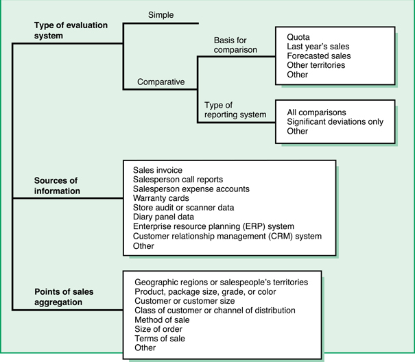
Type of Evaluation System
The first major decision related to sales analysis is the type of evaluation system to use. The type of evaluation system determines how the sales analysis will be conducted. Will it be a simple sales analysis, or a comparative analysis? When it is to be a comparative analysis, two additional questions arise: (1) What is to be the base for the comparison? (2) What type of reporting and control system is to be used?
In a simple sales analysis, the facts are listed and not measured against any standard. In a comparative analysis or, as it is sometimes called, a performance analysis, comparisons are made. Consider, for example, the data in Exhibit 5.14. A simple sales analysis would be restricted to the facts in column 1. These figures suggest Dawson sold the most and Barrington the least. A performance analysis would attempt to go beyond the mere listing of sales to determine where they are greatest and poorest—that is, it would try to make comparisons against some “standard.” In Exhibit 5.14, the standard is the quota for each salesperson (column 2), and column 3 provides a performance index for each. This performance index is calculated as the ratio of actual sales to sales quota (PI = S/Q × 100). It suggests Dawson was not the “best” in 2020, but rather Bendt was. In fact, Dawson realized the smallest percentage of total potential as judged by quota.
EXHIBIT 5.14
Differences between simple sales analysis and comparative analysis

Bases for Comparison
The comparison with quota is only one type of comparison that can be made. Quota is one of the most common standards because it is very useful, particularly when quotas have been specified well. However, some firms resort to other bases of comparison for a sales analysis, and management must decide which bases of comparison are best for their particular situation. Options might include (1) this year’s sales versus last year’s sales or the average of a number of prior years’ sales; (2) this year’s sales versus forecasted sales; (3) sales in one territory versus sales in another, either absolutely or in relation to the ratios in prior years; and (4) the percentage change in sales from one territory to another, as compared with last year.
Such comparisons are certainly better than simply viewing raw sales figures, but they are not generally as productive as a “true” performance analysis. In the latter, variations from planned performance are highlighted, and the reasons for such exceptions are isolated.
Type of Reporting System
The other major issue that arises in a comparative sales analysis is the type of reporting and control system to be used. For example, if one relevant comparison is to be sales as a percentage of quota, this statistic would be provided for each salesperson, branch, district, region, customer, product, and every other unit by which sales are to be analyzed. The problem with this is that it can inundate the sales manager with information. To aid the sales manager, the reports can focus on exceptions, or significant deviations from the norm or from budget. Sales managers can then concentrate on the exceptions while having the full profile of comparisons for assessing the significance of what happened.
Sources of Information for Sales Analysis
A second class of major decisions that must be made with respect to sales analysis is what information is to serve as input to the system and how the basic source documents are to be processed. To address this question, the firm first needs to determine the types of comparisons to be made. A comparison with sales in other territories will require fewer documents than a comparison against market potential or quota or against the average sales in the territory for the last five years. The firm also needs to decide the extent to which preparing the sales report should be integrated with preparing other types of reports. These may include inventory or production reports or sales reports for other company units such as other divisions.
Generally, one of the most productive source documents is the sales invoice. From this, the following information can usually be extracted:
- Customer name and location.
- Product(s) or service(s) sold.
- Volume and dollar amount of the transaction.
- Salesperson (or agent) responsible for the sale.
- End use of product sold.
- Location of customer facility where product is to be shipped or used.
- Customer’s industry, class of trade, or channel of distribution.
- Terms of sale and applicable discount.
- Freight paid or to be collected.
- Shipment point for the order.
- Transportation used in shipment.
Other documents provide more specialized output. Some of the more important of these are listed in Exhibit 5.15. As we learned in Chapter 3, CRM systems facilitate the capturing of the customer information referred to in Exhibit 5.15. This customer information can be analyzed and applied to particular sales analysis questions.
EXHIBIT 5.15
Other sources of information for sales analysis

Software that links processes such as bid estimation, order entry, shipping, billing systems, and other work processes is called an enterprise resource planning system, or ERP. Boeing uses an ERP system to price out airplanes. Each airline and private customer who buys a jet will fit out each jet differently. As a result, the salesperson’s proposal has to account for each different item in order to derive a price. Plus, commission has to be paid on the sale, parts have to be ordered for manufacturing, delivery has to be scheduled—and the ERP helps manage all of these functions. As with CRM, the information generated through enterprise software is an invaluable resource in sales analysis. Yet, ERP implementation must be done properly in order to optimize its value added to the sales organization. The Innovation box on p. 179 illustrates several important risks of ERP implementation.
Type of Aggregation of Information to Be Used in Sales Analysis
The third major decision management must confront when designing a sales analysis is which variables will serve as points of aggregation. Without such categories, the firm would be forced to analyze every transaction in isolation or would need to look at sales in the total aggregate. The latter is not particularly informative, and the former is almost impossible. The most common and instructive procedure is to assemble and tabulate sales by some appropriate groupings, such as these:
- Geographic regions such as states, counties, regions, or salespeople’s territories.
- Product, package size, grade, or color.
- Customer or customer size.
- Market, including class of customer, end use, or channel of distribution.
- Method of sale, including mail, telephone, or direct salespeople.
- Size of order.
- Financial arrangement such as cash or charge.
The classes of information a company may use depend on such things as its size, the diversity of its product line, the geographic extent of its sales area, the number of markets and customers it serves, and the level and type of management for which the information is to be supplied. The firms with a product management form of organization, for example, would be interested in sales by product groups. Product managers might focus on territory-by-territory sales of their products. On the other hand, sales managers will likely be much more interested in territory and customer analyses and only secondarily interested in the territory sales broken out by product.
These sales breakdowns are not necessarily mutually exclusive in that the manager has to choose only one approach. Rather, sales analyses are most productive when they are done hierarchically, in the sense that one breakdown is carried out within another category. The categories are treated simultaneously instead of separately. For example, the analysis may end up showing that customer XYZ in the western region purchased so many units each of products A, B, C, and D. This illustrates a territory, customer, and product hierarchical breakdown.
The advantage of hierarchical breakdowns is illustrated later. For now, you should know that the typical sales analysis results not in a single report but in a family of reports, each reflecting a different level of aggregation, tailored to the person receiving it. Exhibit 5.16, for example, shows the types of sales reports used in a consumer food products company.
EXHIBIT 5.16
Sales reports in a consumer food products company
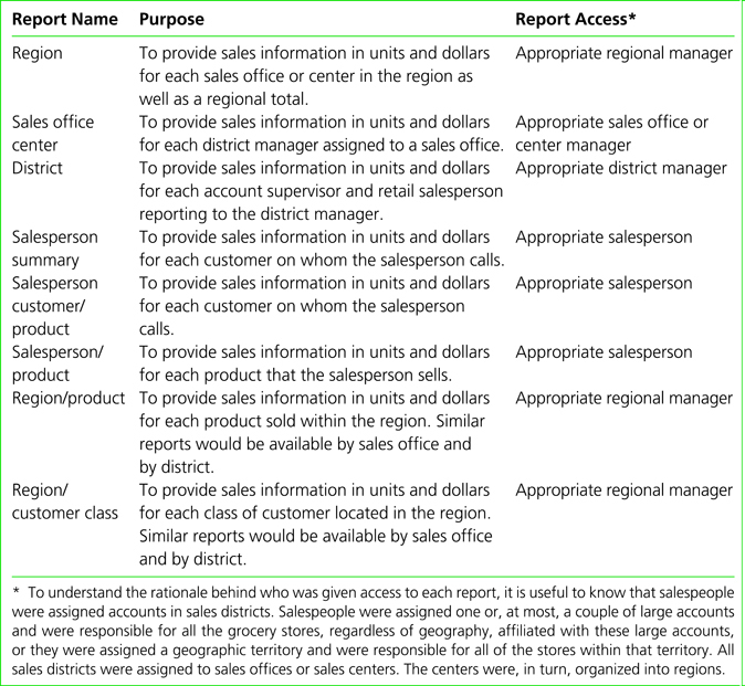
Illustration of a Hierarchical Sales Analysis
To illustrate some relevant comparisons and the process used in conducting a sales analysis, consider the example data in Exhibit 5.17 for the XYZ Company. Again, this is a U.S.-centric example but the process can be utilized in any locale in the world for which sufficient information is available. Let’s assume the XYZ Company previously determined its sales are highly correlated with population, income, and the general level of retail sales. As such, it has used the Buying Power Index (BPI) to determine each region’s market potential and has then multiplied these potentials by the company’s expected market share to generate the regional quotas in Exhibit 5.17.
EXHIBIT 5.17
Sales and sales quotas for XYZ company

Note that although the annual quota was $420 million, total sales in all regions were $421.23 million. Not only has the total company met quota, but also so have most of the regions. The performance index, the ratio of sales to quota, is greater than 100 for five regions. Four regions fell short of their targets, but three of those came very close. Only the east north-central region fell short by any substantial amount (–5.12 percent), but it still had the highest absolute dollar value of sales of any of the major regions. Many sales managers might be tempted from this to assume all is well. At the most, they might send a letter to the manager of the east north-central region, urging him or her to push the salespeople in the region to do better. However, the best approach is to generate the sales breakdown for the east north-central region shown in Exhibit 5.18. The state quotas were determined by multiplying the BPI total U.S. percentages for each state by the $420 million total forecasted sales. In many cases, the firm might wish to convert each percentage to a percentage of the region rather than of the United States as a whole. Thus, the percentage for Illinois would be (6.0037 ÷ 20.1419) × 100 = 29.8. This percentage would then be applied to the $8.60 million quota for the region to get the quota for Illinois. Although the result is the same, this second alternative provides a clearer picture of the concentration of demand in the region. The benefit of this approach holds particularly when one works with smaller and smaller units of analysis.
EXHIBIT 5.18
Sales breakdown for east north-central region of XYZ company
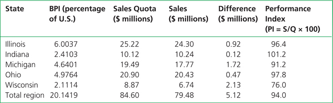
Exhibit 5.18 shows a problem with sales throughout the region. Referring to the “Performance Index” columns, only the sales representatives in Indiana exceeded quota, and then only slightly. Note that the deviations about quota are larger than they were in Exhibit 5.17. This generally happens as one moves to smaller units of analysis. With larger aggregates—for example, regions versus states—the statistician’s law of large numbers seems to apply in that the pluses and minuses about quota tend to balance each other. Thus, the performance indexes in the larger analysis tend to be closer to 100. A smaller deviation from quota should initiate further investigation when the analysis is based on large aggregates (regions) rather than on small ones (salespeople). Although some negative deviation in actual sales from standard is evident in Exhibit 5.18 among four of the five states, the deviation in Wisconsin is most pronounced. Only 76 percent of the quota was realized here.
Again, after examining this Wisconsin information, it would be very easy for a sales manager to take some immediate action. However, the savvy manager would recognize that more analysis is needed to uncover what is truly going on. The sales manager should review the tabulation of sales by sales representatives in the Wisconsin district. The eight areas into which the state is divided are shown in Exhibit 5.19, and the results of the tabulation of sales by representative are shown in Exhibit 5.20. Sales are below quota in all sales areas in the state. This suggests that something may be fundamentally wrong. Perhaps economic conditions are poor and unemployment is high; perhaps competition is more intense than in other areas; or perhaps a problem exists with sales force morale and motivation. Although numerous plausible explanations exist for the sales manager to check, the core problem seems to be Hutchins. If he had done as well as the other sales reps in the state, sales for the district would have been much closer to target. The problem is particularly acute because Hutchins has the prime Milwaukee market for a sales territory. Before taking action about Hutchins, the sales manager should examine more specific information on his sales. Hutchins’s sales by product are shown in Exhibit 5.21. Hutchins is below quota on the entire product line, but seems to be having the most problem with coffee makers and blenders/mixers/food processors.
EXHIBIT 5.19
XYZ company sales territories in Wisconsin
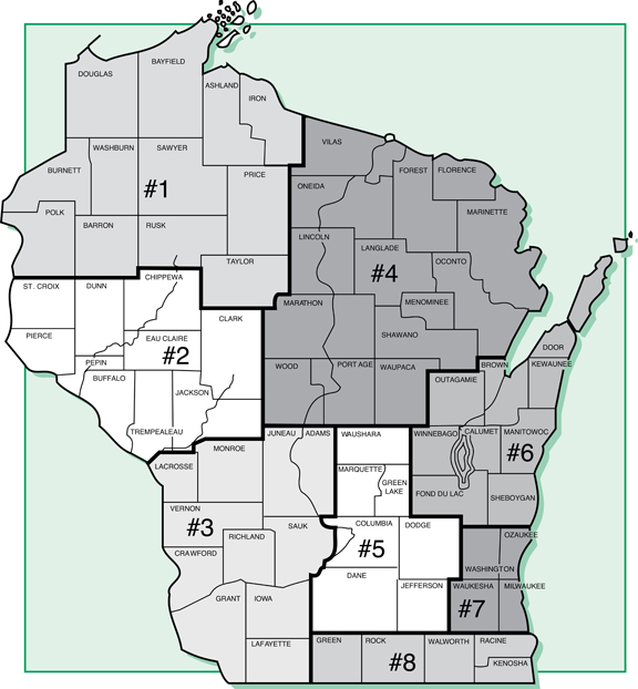
EXHIBIT 5.20
Sales by representative in the Wisconsin district of XYZ company

EXHIBIT 5.21
Hutchins’s sales by product
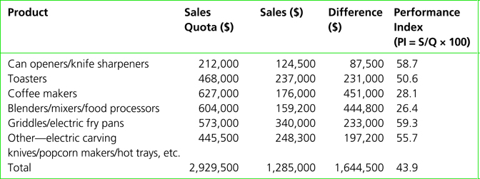
So the fundamental question for the sales manager is the following: Is the problem Hutchins or these products? A further analysis of sales of these products by customer indicated the problem was concentrated among large department store buyers. Furthermore, the problem was not unique to Hutchins but was common to all reps in the east and west north-central regions. A major competitor had been attempting to improve its position in the north-central region through a combination of heavy advertising and purchase rebate offers on these products. This problem had been obscured in other sales territories because sales of other products had compensated for lost sales in coffee makers and blenders/mixers/food processors. Hutchins’s sales of other products did not make up the deficit. The problem was compounded by an economic slowdown in the metal-working industry, a big employer in the Milwaukee area.
The Iceberg Principle
Our sales analysis indicates that the problem is not Hutchins; rather, it is the special competitive situation in the north-central region. This situation would not have come to light without this detailed sales analysis. One important principle illustrated by the preceding example is that aggregate figures can be deceiving. Another principle is that small, visible problems are often symptoms of large, unseen problems. The phenomenon has been linked to an iceberg—the iceberg principle, so named because only about 10 percent of an iceberg’s mass is above the water level (analogous to the symptoms of a problem). The other 90 percent of the berg is below the surface (analogous to the real problem), and not always directly below the tip either. The submerged portion can be very dangerous to ships. So it is with much sales, marketing, and business data. Real problems are often obscured by visible symptoms.
The typical business engages in many varied activities and collects large volumes of data to support these activities. Thus, it is very common for difficulties or problems in one area to be submerged. The sales manager in our example would have succumbed to a misperception of the problem had the original aggregate sales analysis in Exhibit 5.17 been the stopping point. At that point, on the surface all appeared basically calm and peaceful, but more careful analysis revealed submerged problems with jagged edges that would continue to suboptimize business results if they are not attended to properly. Those analyzing the information that is collected need to be especially wary that the summaries they produce by aggregating and averaging data do not hide more than they reveal.
The iceberg principle is pervasive. The 80:20 rule or concentration ratio discussed earlier is one manifestation of it. Often, the concentration of sales within certain territories, products, or customers hides specific weaknesses. More than one company has shown satisfactory total sales, but when the total was subdivided by territories, customers, and products, serious weaknesses were uncovered.
The preceding sales analysis example also vividly illustrates the difference between a simple sales analysis and a comparative sales analysis, as well as the advantages of the latter. The simple raw sales analysis would have focused on the raw sales data in Exhibit 5.17—it would not have examined the differences from quota. In fact, simple sales analysis probably would not have generated any detailed investigation of the east north-central region because sales there were higher than in any other region. The comparison with quota, however, emphasized that the potential in this region was also greater than in any other and the firm was failing to get its share. The comparative analysis triggered the more intensive investigation and isolated the primary reason for the sales shortfall. The execution of the process depended on having sales quotas available on a very small basis. They had to be available by customer, by product, and by salesperson or the problem would never have come to light.
Quotas are sometimes difficult to generate on such a small basis. In our example, it was possible because detailed geographic statistics on the BPI were available. In situations where other data should be used, they need to be available by small geographic area. That is one reason the sales planning and sales evaluation questions are so intertwined. One must keep in mind the questions of evaluation and the comparisons needed when designing sales territories and sales quotas.
The Isolate-and-Explode Principle
Another concept the example illustrates is the principle of isolate and explode, in which the most significant discrepancies between actual and standard are identified, or isolated, and then examined in detail, or exploded. The detail this explosion reveals is then analyzed, the most significant discrepancies are again isolated, and these are exploded. The process continues until the “real” problems are isolated. Thus, in the example, the following were all isolated and exploded in turn: the east north-central region, the Wisconsin district, Hutchins’s sales by product, and Hutchins’s product sales by customer.
An alternative would have been to have masses of data available to the sales manager initially. For example, the information system could have supplied the sales manager with the detailed tabulations of sales by each salesperson of each product to each customer in the beginning. More than likely, such a tabulation would go unused because of its size and the time it would take to decipher its contents. The isolate-and-explode principle makes the task manageable. The sales manager can quickly localize trouble spots by focusing on the most substantial exceptions from standard and then hone in more efficiently on an effective cure.
The principle can also be used to isolate exceptional performances for the clues they might provide to what the firm is doing right. Investigating why the east south-central region was 5.1 percent over quota when the entire company was only 0.3 percent over quota might suggest effective competitive strategies and identify best practices that can be duplicated in other sales units.
The isolate-and-explode principle assumes the company’s information system can provide sales data hierarchically. In the example, the sales manager could secure data broken out by customer, by product, by sales rep, by district, and by region. The breakdowns resemble a tree: Total U.S. sales are the trunk, regions are the main limbs, districts the next branches, and so on. Further, all combinations of these branches are possible. For example, it is possible to do a study by product and territory, or by customer and product. These alternative types of analysis can also be productive, as can simple one-way categorizing of sales data. The simple tabulation of sales by product, for example, is very useful in showing a firm’s product line strengths. Similarly, the simple tabulation of sales by major classes of customers is often informative about the company’s market strengths. Keep in mind that these sales analyses are diagnostics, not decision rules. They do not tell the manager what to do but only offer clues as to causes of problems. And sales analyses are only part of the story.
SUMMARY
We have seen in the chapter that sales managers perform a vital role in the process of both using and generating information. The sales forecasts, quotas, territories, and sales analyses developed under the leadership of sales managers touch most every operational aspect of a firm. Aspects of organizational success at many levels are affected by the proficiency of sales managers in performing these information management roles. From the profitability brought by strategic marketing plans when a forecast proves accurate, to the satisfaction of a customer when a sales territory design allows for proper coverage, to the rewards afforded a salesperson for quota attainment—all these outcomes reflect on the sales manager’s capability to effectively use information in the job.
Because of this impact, sales managers have a vested interest in becoming as proficient as possible in the information management aspect of their job as described in this chapter. The greater their mastery of these important facets of the position, the greater will be not only their own professional success but also the success of the firm and its salespeople.
KEY TERMS
market potential
sales potential
sales forecast
sales quotas
subjective forecasting methods
user expectations
sales force composite
jury of executive opinion
Delphi technique
objective forecasting methods
market test
time-series analysis
moving average
exponential smoothing
decomposition
statistical demand analysis
scenario planning
North American Industry Classification System (NAICS)
buying power index (BPI)
sales volume quotas
activity quotas
financial quotas
sales force deployment
breakdown method
workload method
incremental method
account analysis
sales analysis
80:20 principle
enterprise resource planning (ERP)
Buying Power Index (BPI)
iceberg principle
isolate and explode
BREAKOUT QUESTIONS
- A common problem faced by those responsible for making sales forecasts is “selling” the predictions to others such as the vice presidents of marketing, production, and human resources, and to the CEO or the CFO. These parties hesitate to use forecasts that can have major implications, especially if they are wrong, on their functional area. What can those responsible for sales forecasting do to better sell their results to management? What forecasting guidelines should be followed to improve the predictions?
- A survey of local business firms to determine how they forecast sales will produce a variety of answers. Some will claim they do not use any formal techniques to forecast sales. You know they must be using some approach, no matter how loosely defined. How do you know a business firm is making a sales forecast? What are the implications of not making a sales forecast?
- For the following products, indicate what factor(s) you would use to estimate market potential:
- Yoplait yogurt
- Rolex watches
- Apple iPads
- Toro power riding lawnmowers
- Ektelon racquetball racquets
- Nicole Miller designer ties
- SWATCH watches
- Tylenol
- Mary Kay cosmetics
- To estimate market potential for the garden tractor division of the M–F Implement Co., Mark Haynes, the statistician, estimated the following relationship using multiple regression analyses:
Using data for 2014–2020, R2 = 65.0 was obtained. Should this method be used to predict market potential?
- A new cake mix is to be introduced by Miracle Foods. To develop territory potentials, a corollary index has been proposed. The index contains several factors, such as income, population, and retail food sales. Can you justify these factors? Does it make sense to use retail food sales, which means cake sales are a function of food sales?
- Once a quarter, every six months, or annually, each salesperson should estimate the buying potential of each account for each major product or product line. Such a request usually causes the sales force to panic. What goals are likely to be achieved by having the sales force participate in sales forecasting? What are the potential pitfalls, if any? How could those pitfalls be overcome?
- Most sales managers hesitate to modify sales territories unless supported by compelling reasons. Likewise, sales managers are reluctant to make major changes in the sales compensation package. On the other hand, reassigning salespeople from one territory to another is fairly common and often reflects a form of promotion. One expert contends that if a company’s sales force knows the territory too well, then it’s time to reassign territories. What are the pros and cons of this approach? What factors related to the salesperson, the company, and the external environment might drive a company to reassign a sales territory?
- The chapter describes the process to follow to develop territories. After territories have been developed, changes may occur that indicate the territories need to be realigned. What changes can you identify that indicate the need for realignment? How would you go about the process of realigning territories? How would you implement the changes?
- In the typical case, management by exception leads to a close examination of below-par situations. Only sales representatives who are not meeting objectives, products that are not selling according to expectations, and customers who are not buying products as predicted are carefully reviewed to determine corrective action. What arguments can be advanced for conducting a close examination of the opposite, above-par situations?
- The use of scanner data collected at the time of checkout in supermarkets has increased dramatically in sales analysis. One company has recruited families nationwide to participate in a panel study. When a shopper enters the checkout lane, he or she gives the clerk a plastic card that is passed over the scanner. All items purchased that are scanned are recorded in the shopper’s diary. Oscar Mayer, a Wisconsin-based producer of meat, turkey, and seafood, has used different advertising campaigns in several markets. Oscar Mayer analyzes scanner data to determine which ad campaign was most effective. How else could Oscar Mayer and other manufacturers use scanner data? Of what value would scanner data be to salespeople for a company such as Oscar Mayer? To food retailers? What are other industries that could benefit from the same type of data?
- The Recall Computer Co. has six territories, each represented by one salesperson. After extensive planning, the company determines that each territory would be expected to achieve the following percentages of total company sales for 2020:
Territory 1
27%
Territory 2
15%
Territory 3
18%
Territory 4
12%
Territory 5
20%
Territory 6
8%
These figures are used as the standard for comparing each sales representative’s actual 2020 sales. The company projected sales for 2020 of $18,500,000. Determine which sales representative’s territory had the best performance by using the performance index, if the actual sales for 2020 in each territory were $5,425,000, $3,205,000, $3,710,000, $2,400,000, $3,900,000, and $2,000,000, respectively, for territories 1–6.
- In planning a sales analysis system, one must consider that information needs vary from district sales manager to regional sales manager to vice president of sales. Give specific examples of how information needs vary among managers at these levels.
- Ethical Question. JUS-GRA Industries is an automotive aftermarket parts distributor based in Munich, Germany. As VP of sales for JUS-GRA industries you have been tasked with opening and staffing the first new sales office for the company’s Asian operations, which are forecast to grow nicely over the next several years. Based in Tokyo, one of the challenges of this region are the large distances that must be traveled by air to call on customers in far flung locations like Seoul, Shanghai, Kuala Lumpur, Singapore, and other key cities that JUS-GRA would like to open for business. As you consider assigning salespeople to this new region you are very mindful of these travel demands along with other inherent challenges of opening up in a new region of the world. At the same time, one of your best longtime salespeople in Germany—Angelika Krafft, who is also a close family friend—has asked you if she could be moved to this new area. Angelika sees this as an opportunity to gain visibility in the company and show what she can do. You know, however, that she has a family with three children aged 11–16 and that the demands of the new job may put pressure on her family and her spouse. How would you handle her request? Explain your decision.
LEADERSHIP CHALLENGE: A QUOTA BY ANY OTHER NAME
Ralph Dickerson knew an adjustment was needed. In more than 20 years with Bright Right Plastics, he had been around for many changes, and as director of sales for the company, he had initiated a number on his own. Now Ralph knew that he had to reevaluate the quota system that had been used at Bright Right for more than 15 years.
The system had been revised years ago to focus the sales force on financial goals, specifically sales volume. At the time, business was slow and senior management had wanted salespeople to drive sales for the company. It had worked as the company prospered and was now enjoying great success. Selling to large hardware stores, the company had built a reputation as a good supplier of quality plastic fittings and joints in the retail plumbing industry. At the same time, many aspects of the business environment had changed since the quota system was last revised. Most notably, foreign competitors had come in offering competitive prices and better service. Several of Bright Right’s old competitors had been driven out of business, and Ralph knew that part of the problem was the quota system in place at the company.
Essentially, the system in place was based on sales volume. As it had evolved the system focused on unit sales. It involved a complex plan that allowed each salesperson to set unit sales goals for every product in the company’s large inventory. Senior management considered quotas a critical element in their strategic planning. At the same time, they were used as motivational tools for the sales force. Each overall quota was set high, but within that the salesperson could develop individual product quotas based on his or her customer’s needs.
The problem, as Ralph saw it, was that customers wanted greater coordination and support from their suppliers. Specifically, customers like Home Depot and Lowe’s wanted salespeople to offer product demonstrations to their own sales force as well as help in arranging displays for the products. Ralph had heard complaints that Bright Right salespeople were less interested in doing these kinds of activities than salespeople from other companies. Unfortunately, he had heard these complaints for several years and was concerned they might be losing business, or soon would be.
He sat in his office pondering his next move. The CEO of the company had set up a meeting for tomorrow to discuss this issue and was looking to Ralph for answers.
Questions
- What are the advantages and disadvantages of a sales volume-based quota system?
- What are the advantages and disadvantages of an activity-based quota system?
- What quota system would you recommend Ralph present to the CEO and why? What challenges would Ralph face in implementing your recommendation?
ROLE-PLAY: BLUE TERN MILLS—PART B
Situation
This situation is a continuation of the situation presented in the Chapter 4 Role-Play. Go back and read that Role-Play and your notes from it to refamiliarize yourself with the scenario.
Agnes, Alan, and Penny have now had their meeting and have proposed a new sales force organization scheme for Blue Tern Mills postacquisition of the Hello line of healthy grain products. It is now time to begin the process of developing a sales forecast for the first year of operation of the combined companies. In order to begin this process, Agnes calls another meeting of the three for a few weeks later.
In advance of the meeting, she asks that each person come prepared with a set of notes listing their proposed combination of forecasting methods to employ along with their rationale for why each should be a part of the final approach to determining this first-year forecast. As you prepare these notes, keep in mind that especially this first year the forecast will be tricky because it will be difficult to determine in advance the full impact of the transition of the Hello line from the manufacturer’s representatives to Blue Tern’s own sales force, with the new organization scheme for it you developed earlier. Clearly, multiple methods of forecasting should be applied to reach a final forecasting decision and information will have to be effectively sourced and utilized from both firms.
The purpose of the meeting is to settle on methods to be employed in developing the first-year forecast, justify those methods, and list information needed and the sources of that information.
Characters in the Role-Play
Agnes Klondyke, chief sales officer (CSO) for Blue Tern Mills
Alan Knorr, West Coast sales manager for Blue Tern Mills
Penny Pugsley, currently the director of sales for Hello Healthy Grain Foods and soon to be East Coast sales manager for Blue Tern Mills (note that Penny’s job at Hello has been to supervise its network of manufacturers’ representatives—Hello does not have its own sales force).
Assignment
Break into groups of three, with one student playing each character. It doesn’t matter what the actual gender mix of your group is. Before you stage the meeting among Agnes, Alan, and Penny, work separately to come up with the information required: your ideas for methods to be employed in developing the first-year forecast, justification for those methods, information that will be needed to drive your selected methods, and the sources of that information. Then get together and role-play the meeting. Share your ideas, especially discussing the pros and cons of different forecasting approaches proposed. After the discussion, come to agreement among yourselves on what will be the best mix of forecasting approaches, given the unique situation in the first year after the acquisition, and specify the needed information and sources. Note that you are not developing a forecast in the meeting—you are simply deciding on what approaches are to be used, why, and what information is needed.
MINICASE: LASTING IMPRESSIONS
Lasting Impressions is a small Orlando, Florida, company that provides trade-show marketing solutions to customers of all sizes. The company offers to design a plan for trade-show exhibiting from start to finish, including developing a pre- and postevent marketing plan and branding strategy, creating the exhibit booth and corresponding collateral support materials, packaging and shipping all trade-show materials, and providing boothmanship training services.
Founded by CEO Rajiv Dembla in 2006, the company focuses its own sales efforts on customers within the state of Florida and has a team of four account executives—Mary Beth, Suzanne, Franco, and Syl—who act as the salespeople for the organization. Rajiv relies on the same territory design that he has for the past several years, in which he divides the state geographically into four equal-size regions, and the account executives are responsible for the cities within their respective region.
Rajiv is not an especially quantitative manager by nature, but he did acknowledge the need to do a sales forecast for the upcoming 2020–21 fiscal year. He used the sales force composite method by asking his account executives how much each expected to sell during the coming year and then totaling those estimates. This type of method has worked for the company in the past, but Rajiv is concerned that Syl acts in the spirit of the marketing adage “underpromise and overdeliver” by intentionally underestimating his sales expectations so that his quota will be lower. To be safe, Rajiv also determined the sales forecast by taking a moving average of the previous four years of sales (see Table FY 2020-21 Forecasted Sales and Quotas).
Account Executive |
Forecasted Sales |
Quota |
Mary Beth |
$180,000 |
$200,000 |
Suzanne |
180,000 |
200,000 |
Franco |
180,000 |
200,000 |
Syl |
180,000 |
200,000 |
Total |
$720,000 |
$800,000 |
Based on an average of these two sales forecasts, Rajiv set out to develop the yearly sales quota for each of his account executives. As he usually did, he kept the quota as simple as possible by basing it on gross dollars brought into the firm from sales, and he made it equal for each account executive. To ensure that his sales team is aggressive, he set the quotas slightly higher than the forecasted sales. As further motivation, Rajiv put 25 percent of each account executive’s compensation in the form of a bonus for meeting or beating sales volume quotas.
John Cook, Rajiv’s executive assistant, is more sensitive to the needs of the staff than Rajiv and tends to be the one that people talk to freely. Mary Beth complains to him privately, “This quota system does not reward—and even punishes—me for doing what I do best, building relationships with customers through in-person consultations, field demonstrations, and attending trade-show events to ensure everything goes smoothly.” She finds these activities invaluable for serving the customer and keeping her pipeline of business full in the long term, but they do not necessarily generate sales volume in the short term.
While Suzanne tells John, “I have no problem with the quota because my territory includes the home city of Orlando. I know all of the businesses there and have no problem generating sales,” Franco comes to John upset. His region includes Tallahassee, Pensacola, and the rest of the Florida Panhandle, which is more rural, is farther away from home, and has fewer businesses. As a result, he says, “I am miserable! I can’t meet these unfair quotas!”
Syl tells John, “I have the same problem generating sales at times in my north-central Florida territory because there are fewer large cities. But,” he whispers with a smile, “I don’t worry about it. I recommend more expensive trade-show supplies and services to my customers at the end of the fiscal year to boost my short-term sales. And if I need more sales to meet my quota, I just do some creative accounting and record sales numbers for this year which should come due at the beginning of next year. It works every time.”
John is in a quandary. He normally keeps the staff complaints confidential, but in this case he feels like he needs to tell Rajiv that all is not well at Lasting Impressions.
Questions
- Based on the facts given, evaluate Rajiv’s territory design. What other basic control unit might Rajiv have used besides cities? Why?
- What other forecast method(s) should Rajiv have used besides the sales force composite moving average? Why?
- What type of sales quota did Rajiv use? Did he set the appropriate quota level? Why or why not?