Theme 1: Data
R is an object-oriented language; that means that it deals with named objects. Most often these objects are the data that you are analyzing. This theme deals with making, getting, saving, examining, and manipulating data objects.
Topics in this Theme
- Data Types
- Creating Data
- Importing Data
- Saving Data
- Viewing Data
- Summarizing Data
- Distribution of Data
Commands in this Theme:
Data Types
R recognizes many kinds of data, and these data can be in one of several forms. This topic shows you the commands relating to the kinds of data and how to switch objects from one form to another.
What’s In This Topic:
- The different types/forms of data objects
- Creating blank data objects
- Switching data from one type to another
- How to tell what type an object is
Types of Data
Data can exist as different types and forms. These have different properties and can be coerced from one type/form into another.
Command Name
arrayAn array is a multidimensional object.
Common Usage
array(data = NA, dim = length(data), dimnames = NULL)Related Commands
Command Parameters
| data = NA | A vector to be used to create the array. Other objects are coerced to form a vector before making the array. |
| dim = length(data) | The dimensions of the array as a vector. A vector of 2 sets row and column sizes, respectively. |
| dimnames = NULL | A list of names for each dimension of the array. The default, NULL, creates no names. |
Examples
  ## Simple arrays
> array(1:12) # Simple 12-item vector
 [1]  1  2  3  4  5  6  7  8  9 10 11 12

> array(1:12, dim = 12) # Set length explicitly
 [1]  1  2  3  4  5  6  7  8  9 10 11 12

> array(1:12, dim = 6) # Can set length to shorter than data
[1] 1 2 3 4 5 6

> array(1:12, dim = 18) # Longer arrays recycle values to fill
 [1]  1  2  3  4  5  6  7  8  9 10 11 12  1  2  3  4  5  6

> array(1:24, dim = c(3, 4, 2)) # A 3-dimensional array
, , 1

     [,1] [,2] [,3] [,4]
[1,]    1    4    7   10
[2,]    2    5    8   11
[3,]    3    6    9   12

, , 2

     [,1] [,2] [,3] [,4]
[1,]   13   16   19   22
[2,]   14   17   20   23
[3,]   15   18   21   24

  ## Arrays with names
  ## A vector
> array(1:12, dim = 12, dimnames = list(LETTERS[1:12]))
 A  B  C  D  E  F  G  H  I  J  K  L
 1  2  3  4  5  6  7  8  9 10 11 12

  ## A matrix
> array(1:12, dim = c(3, 4), dimnames = list(letters[1:3], LETTERS[1:4]))
  A B C  D
a 1 4 7 10
b 2 5 8 11
c 3 6 9 12

  ## A 3D array (3 row by 4 column)*2
> array(1:24, dim = c(3, 4, 2), dimnames = list(letters[1:3], LETTERS[1:4],
 month.abb[1:2]))
, , Jan

  A B C  D
a 1 4 7 10
b 2 5 8 11
c 3 6 9 12

, , Feb

   A  B  C  D
a 13 16 19 22
b 14 17 20 23
c 15 18 21 24
Command Name
characterData in text form (not numbers) is called character data. The command creates a blank data object containing empty text data items.
Common Usage
character(length = 0)Related Commands
Command Parameters
| length = 0 | Sets the length of the new vector to be created. The default is 0. |
Examples
  ## Make a 5-item vector containing blank entries
> (newchar = character(length = 5))
[1] "" "" "" "" ""
Command Name
data.frameA data.frame is a two-dimensional, rectangular object that contains columns and rows. The columns can contain data of different types (some columns can be numbers and others text). The command makes a data frame from named objects.
Common Usage
data.frame(..., row.names = NULL,
           stringsAsFactors = default.stringsAsFactors())
Related Commands
Command Parameters
| ... | Items to be used in the construction of the data frame. Can be object names separated by commas. |
| row.names = NULL | Specifies which column will act as row names for the final data frame. Can be an integer or character string. |
| stringsAsFactors | A logical value, TRUE or FALSE. Should character values be converted to factor? Default is TRUE. |
Examples
  ## Make some data
> abundance = c(12, 15, 17, 11, 15, 8, 9, 7, 9)
> cutting = c(rep("mow", 5), rep("unmow", 4))

  ## Make data frame with cutting as factor (the default)
> graze = data.frame(abundance, cutting)

  ## Make data frame with cutting as character data
> graze2 = data.frame(abundance, cutting, stringsAsFactors = FALSE)

  ## Make row names
> quadrat = c("Q1", "Q2", "Q3", "Q4", "Q5", "Q6", "Q7", "Q8", "Q9")

  ## Either command sets quadrat to be row names
> graze3 = data.frame(abundance, cutting, quadrat, row.names = 3)
> graze3 = data.frame(abundance, cutting, quadrat, row.names = "quadrat")
Command Name
factorThis command creates factor objects. These appear without quotation marks and are used in data analyses to indicate levels of a treatment variable.
Common Usage
factor(x = character(), levels, labels = levels)Related Commands
Command Parameters
| x = character() | A vector of data, usually simple integer values. |
| levels | Optional. A vector of values that the different levels of the factor could be. The default is to number them in alphabetical order. |
| labels = levels | Optional. A vector of labels for the different levels of the factor. |
Examples
  ## Make an unnamed factor with 2 levels
> factor(c(rep(1, 5), rep(2, 4)))
[1] 1 1 1 1 1 2 2 2 2
Levels: 1 2

  ## Give the levels names
> factor(c(rep(1, 5), rep(2, 4)), labels = c("mow", "unmow"))
[1] mow   mow   mow   mow   mow   unmow unmow unmow unmow
Levels: mow unmow

  ## Same as previous
> factor(c(rep("mow", 5), c(rep("unmow", 4))))

  ## Change the order of the names of the levels
> factor(c(rep(1, 5), rep(2, 4)), labels = c("mow", "unmow"), levels = c(2,1))
[1] unmow unmow unmow unmow unmow mow   mow   mow   mow
Levels: mow unmow
Command Name
ftableCreates a “flat” contingency table.
Command Name
integerData objects that are numeric (not text) and contain no decimals are called integer objects. The command creates a vector containing the specified number of 0s.
Common Usage
integer(length = 0)Related Commands
Command Parameters
| length = 0 | Sets the number of items to be created in the new vector. The default is 0. |
Examples
  ## Make a 6-item vector
> integer(length = 6)
[1] 0 0 0 0 0 0
Command Name
listA list object is a collection of other R objects simply bundled together. A list can be composed of objects of differing types and lengths. The command makes a list from named objects.
Common Usage
list(...)Related Commands
Command Parameters
| ... | Objects to be bundled together as a list. Usually named objects are separated by commas. |
Examples
  ## Create 3 vectors
> mow = c(12, 15, 17, 11, 15)
> unmow = c(8, 9, 7, 9)
> chars = LETTERS[1:5]

  ## Make list from vectors
> mylist = list(mow, unmow, chars) # elements are unnamed

  ## Make list and assign names
> mylist = list(mow = mow, unmow = unmow, chars = chars)
Command Name
logicalA logical value is either TRUE or FALSE. The command creates a vector of logical values (all set to FALSE).
Common Usage
logical(length = 0)Related Commands
Command Parameters
| length = 0 | The length of the new vector. Defaults to 0. |
Examples
  ## Make a 4-item vector containing logical results
> logical(length = 4)
[1] FALSE FALSE FALSE FALSE
Command Name
matrixA matrix is a two-dimensional, rectangular object with rows and columns. A matrix can contain data of only one type (either all text or all numbers). The command creates a matrix object from data.
Common Usage
matrix(data = NA, nrow = 1, ncol = 1, byrow = FALSE, dimnames = NULL)Related Commands
Command Parameters
| data = NA | The data to be used to make the matrix. Usually a vector of values (numbers or text). |
| nrow = 1 | The number of rows into which to split the data. Defaults to 1. |
| ncol = 1 | The number of columns into which to split the data. Defaults to 1. |
| byrow = FALSE | The new matrix is created from the data column-by-column by default. Use byrow = TRUE to fill up the matrix row-by-row. |
| dimnames = NULL | Sets names for the rows and columns. The default is NULL. To set names, use a list of two (rows, columns). |
Examples
  ## Make some data
> values = 1:12 # A simple numeric vector (numbers 1 to 12)

  ## A matrix with 3 columns
> matrix(values, ncol = 3)
     [,1] [,2] [,3]
[1,]    1    5    9
[2,]    2    6   10
[3,]    3    7   11
[4,]    4    8   12

  # A matrix with 3 columns filled by row
> matrix(values, ncol = 3, byrow = TRUE)
     [,1] [,2] [,3]
[1,]    1    2    3
[2,]    4    5    6
[3,]    7    8    9
[4,]   10   11   12

  ## Make some labels
> rnam = LETTERS[1:4] # Uppercase letters A-D
> cnam = letters[1:3] # Lowercase letters a-c

  ## Set row and column names in new matrix
> matrix(values, ncol = 3, dimnames = list(rnam, cnam))
  a b  c
A 1 5  9
B 2 6 10
C 3 7 11
D 4 8 12
Command Name
numericData that are numeric are numbers that may contain decimals (not integer values). The command creates a new vector of numbers (all 0).
Common Usage
numeric(length = 0)Related Commands
Command Parameters
| length = 0 | Sets the number of items to be in the new vector. Defaults to 0. |
Examples
  ## Make a 3-item vector
> numeric(length = 3)
[1] 0 0 0
Command Name
rawData that are raw contain raw bytes. The command creates a vector of given length with all elements 00.
Common Usage
raw(length = 0)Related Commands
Command Parameters
| length = 0 | Sets the length of the new vector. Defaults to 0. |
Examples
  ## Make a 5-item vector
> raw(length = 5)
[1] 00 00 00 00 00
Command Name
tableThe table command uses cross-classifying factors to build a contingency table of the counts at each combination of factor levels.
Related Commands
Command Name
tsA time-series object contains numeric data as well as information about the timing of the data. The command creates a time-series object with either a single or multiple series of data. The resulting object will have a class attribute "ts" and an additional "mts" attribute if it is a multiple series. There are dedicated plot and print methods for the "ts" class.
Common Usage
ts(data = NA, start = 1, end = numeric(0), frequency = 1, deltat = 1,
   ts.eps = getOption("ts.epd"), class = , names = )
Related Commands
Command Parameters
| data = NA | The numeric data. The data can be a vector, a matrix, or a data frame. A vector produces a single time-series, whereas a data frame or a matrix produces multiple time-series in one object. |
| start = 1 | The starting time. Either a single numeric value or two integers. If two values are given, the first is the starting time and the second is the period within that time (based on the frequency); e.g., start = c(1962, 2) would begin at Feb 1962 if frequency = 12 or 1962 Q2 if frequency = 4. |
| end = numeric(0) | The ending time, specified in a similar manner to start. |
| frequency = 1 | The frequency of observation per unit time. Give either a frequency or deltat parameter. |
| deltat = 1 | The fraction of the sampling period between successive observations (so 1/12 would be monthly data). Give either a frequency or deltat parameter. |
| ts.eps = getOption("ts.eps") | Sets the comparison tolerance. Frequencies are considered equal if their absolute difference is less than the value set by the ts.eps parameter. |
| names = | The names to use for the series of observations in a multiple-series object. This defaults to the column names of a data frame. You can use the colnames and rownames commands to set the names of columns (data series) or rows afterwards. |
Examples
  ## A simple vector
> newvec = 25:45

## Make a single time-series for annual, quarterly, and monthly data

> ts(newvec, start = 1965) # annual
Time Series:
Start = 1965
End = 1985
Frequency = 1
 [1] 25 26 27 28 29 30 31 32 33 34 35 36 37 38 39 40 41 42 43 44 45

> ts(newvec, start = 1965, frequency = 4) # quarterly
     Qtr1 Qtr2 Qtr3 Qtr4
1965   25   26   27   28
1966   29   30   31   32
1967   33   34   35   36
1968   37   38   39   40
1969   41   42   43   44
1970   45

> ts(newvec, start = 1965, frequency = 12) # monthly
     Jan Feb Mar Apr May Jun Jul Aug Sep Oct Nov Dec
1965  25  26  27  28  29  30  31  32  33  34  35  36
1966  37  38  39  40  41  42  43  44  45

  ## Make a matrix
> mat = matrix(1:60, nrow = 12)

  ## Make a multiple time-series object, monthly data
> ts(mat, start = 1955, frequency = 12)
         Series 1 Series 2 Series 3 Series 4 Series 5
Jan 1955        1       13       25       37       49
Feb 1955        2       14       26       38       50
Mar 1955        3       15       27       39       51
Apr 1955        4       16       28       40       52
May 1955        5       17       29       41       53
Jun 1955        6       18       30       42       54
Jul 1955        7       19       31       43       55
Aug 1955        8       20       32       44       56
Sep 1955        9       21       33       45       57
Oct 1955       10       22       34       46       58
Nov 1955       11       23       35       47       59
Dec 1955       12       24       36       48       60
Command Name
vectorA vector is a one-dimensional data object that is composed of items of a single data type (all numbers or all text). The command creates a vector of given length of a particular type. Note that the mode = "list" parameter creates a list object. Note also that a factor cannot be a vector.
Common Usage
vector(mode = "logical", length = 0)Related Commands
Command Parameters
| mode = "logical" | Sets the kind of data produced in the new vector. Options are "logical" (the default), "integer", "numeric", "character", "raw" and "list". |
| length = 0 | Sets the number of items to be in the new vector. Default is 0. |
Examples
  ## New logical vector
> vector(mode = "logical", length = 3)
[1] FALSE FALSE FALSE

  ## New numeric vector
> vector(mode = "numeric", length = 3)
[1] 0 0 0

  ## New character vector
> vector(mode = "character", length = 3)
[1] "" "" ""

  ## New list object
> vector(mode = "list", length = 3)
[[1]]
NULL

[[2]]
NULL

[[3]]
NULL
Command Name
xtabsThis command carries out cross tabulation, creating a contingency table as a result.
Altering Data Types
Each type of data (for example, numeric, character) can potentially be switched to a different type, and similarly, each form (for example, data frame, matrix) of data object can be coerced to a new form. In general, a command of the form as.xxxx (where xxxx is the name of the required data type) is likely to be what you need.
Command Name
as.array
as.character
as.data.frame
as.factor
as.integer
as.list
as.logical
as.matrix
as.numeric
as.raw
as.table
as.ts
as.vector
These commands attempt to coerce an object into the specified form. This will not always succeed.
Common Usage
as.character(x)Related Commands
Command Parameters
| x | The object to be coerced to the new form. |
Examples
  ## Make simple data vector
> sample = c(1.2, 2.4, 3.1, 4, 2.7)

  ## Make into integer values
> as.integer(sample)
[1] 1 2 3 4 2

  ## Make into characters
> as.character(sample)
[1] "1.2" "2.4" "3.1" "4"   "2.7"

  ## Make into list
> as.list(sample)
[[1]]
[1] 1.2

[[2]]
[1] 2.4

[[3]]
[1] 3.1

[[4]]
[1] 4

[[5]]
[1] 2.7

  ## Make a matrix of numbers
> matdata = matrix(1:12, ncol = 4)

  ## Coerce to a table
> as.table(matdata)
   A  B  C  D
A  1  4  7 10
B  2  5  8 11
C  3  6  9 12
Command Name
as.data.frameThis command attempts to convert an object into a data frame. For example, this can be useful for cross tabulation by converting a frequency table into a data table.
Testing Data Types
You can determine what sort of data an object contains and also the form of the data object. Generally, a command of the form is.xxxx (where xxxx is the object type to test) is required. The result is a logical TRUE or FALSE.
Command Name
classReturns the class attribute of an object.
Command Name
inheritsTests the class attribute of an object. The return value can be a logical value or a number (0 or 1).
Common Usage
inherits(x, what, which = FALSE)Related Commands
Command Parameters
| x | An R object. |
| what | A character vector giving class names to test. Can also be NULL. |
| which = FALSE | If which = FALSE (the default), a logical value is returned by the command. This value will be TRUE if any of the class names of the object match any of the class names in the what parameter. If which = TRUE, an integer vector is returned that is the same length as what. Each element of the returned vector indicates the position of the class matched by what; a 0 indicates no match. |
Examples
  ## Make an object
> newmat = matrix(1:12, nrow = 3)

  ## See the current class
> class(newmat)
[1] "matrix"

  ## Test using inherits()
> inherits(newmat, what = "matrix")
[1] TRUE

> inherits(newmat, what = "data.frame")
[1] FALSE

> inherits(newmat, what = "matrix", which = TRUE)
[1] 1

> inherits(newmat, what = c("table", "matrix"), which = TRUE)
[1] 0 1

  ## Add an extra class to object
> class(newmat) = c("table", "matrix")
> class(newmat)
[1] "table"  "matrix"

  ## Test again
> inherits(newmat, what = "matrix")
[1] TRUE

> inherits(newmat, what = "data.frame")
[1] FALSE

> inherits(newmat, what = "matrix", which = TRUE)
[1] 2

> inherits(newmat, what = c("table", "matrix"), which = TRUE)
[1] 1 2

> inherits(newmat, what = c("table", "list", "matrix"), which = TRUE)
[1] 1 0 2
Command Name
isDetermines if an object holds a particular class attribute.
Common Usage
is(object, class2)Related Commands
Command Parameters
| object | An R object. |
| class2 | The name of the class to test. If this name is in the class attribute of the object, TRUE is the result. |
Examples
  ## Make an object
> newmat = matrix(1:12, nrow = 3)

> ## See the current class
> class(newmat)
[1] "matrix"

  ## Test using is()
> is(newmat, class2 = "matrix")
[1] TRUE

> is(newmat, class2 = "list")
[1] FALSE

  ## Add an extra class to object
> class(newmat) = c("table", "matrix")
> class(newmat)
[1] "table"  "matrix"

  ## Test again
> is(newmat, class2 = "matrix")
[1] TRUE

> is(newmat, class2 = "list")
[1] FALSE
Command Name
is.array
is.character
is.data.frame
is.factor
is.integer
is.list
is.logical
is.matrix
is.numeric
is.raw
is.table
is.ts
is.vector
These commands test an object and returns a logical value (TRUE or FALSE) as the result.
Common Usage
is.character(x)Related Commands
Command Parameters
| x | The object to be tested. The result is a logical TRUE or FALSE. |
Examples
  ## Make a numeric vector
> (sample = 1:5)
[1] 1 2 3 4 5

  ## Is object numeric?
> is.numeric(sample)
[1] TRUE

  ## Is object integer data?
> is.integer(sample)
[1] TRUE

  ## Is object a matrix?
> is.matrix(sample)
[1] FALSE

  ## Is object a factor?
> is.factor(sample)
[1] FALSE
Creating Data
Data can be created by typing in values from the keyboard, using the clipboard, or by importing from another file. This topic covers the commands used in creating (and modifying) data from the keyboard or clipboard.
What’s In This Topic:
- Use the keyboard to make data objects
- Use the clipboard to transfer data from other programs
- Add extra data to existing objects
- Amend data in existing objects
Creating Data from the Keyboard
Relatively small data sets can be typed in from the keyboard.
Command Name
cThis command is used whenever you need to combine items. The command combines several values/objects into a single object. Can be used to add to existing data.
Common Usage
c(...)Related Commands
Command Parameters
| ... | Objects to be joined together (concatenated); names are separated by commas. |
Examples
  ## Make a simple vector from numbers
> mow = c(12, 15, 17, 11, 15)

  ## Make text (character) vectors
> wday = c("Mon", "Tue", "Wed", "Thu", "Fri")
> week = c(wday, "Sat", "Sun")
Command Name
cbindAdds a column to a matrix.
Command Name
glGenerates factor levels. This command creates factor vectors by specifying the pattern of their levels.
Common Usage
gl(n, k, length = n*k, labels = 1:n, ordered = FALSE)Related Commands
Command Parameters
| n | An integer giving the number of levels required. |
| k | An integer giving the number of replicates for each level. |
| length = n*k | An integer giving the desired length of the result. |
| labels = 1:n | An optional vector of labels for the factor levels that result. |
| ordered = FALSE | If ordered = TRUE, the result is ordered. |
Examples
  ## Generate factor levels
> gl(n = 3, k = 1) # 3 levels, 1 of each
[1] 1 2 3
Levels: 1 2 3

> gl(n = 3, k = 3) # 3 levels, 3 of each
[1] 1 1 1 2 2 2 3 3 3
Levels: 1 2 3

> gl(n = 3, k = 3, labels = c("A", "B", "C")) # Use a label
[1] A A A B B B C C C
Levels: A B C

> gl(n = 3, k = 3, labels = c("Treat")) # All same label plus index
[1] Treat1 Treat1 Treat1 Treat2 Treat2 Treat2 Treat3 Treat3 Treat3
Levels: Treat1 Treat2 Treat3

> gl(n = 3, k = 1, length = 9) # Repeating pattern up to 9 total
[1] 1 2 3 1 2 3 1 2 3
Levels: 1 2 3

> gl(n = 2, k = 3, labels = c("Treat", "Ctrl")) # Unordered
[1] Treat Treat Treat Ctrl  Ctrl  Ctrl
Levels: Treat Ctrl

> gl(n = 2, k = 3, labels = c("Treat", "Ctrl"), ordered = TRUE) # Ordered
[1] Treat Treat Treat Ctrl  Ctrl  Ctrl
Levels: Treat < Ctrl

> gl(n = 3, k = 3, length = 8, labels = LETTERS[1:3], ordered = TRUE)
[1] A A A B B B C C
Levels: A < B < C
Command Name
interactionThis command creates a new factor variable using combinations of other factors to represent the interactions. The resulting factor is unordered. This can be useful in creating labels or generating graphs.
Common Usage
interaction(..., drop = FALSE, sep = ".")Related Commands
Command Parameters
| ... | The factors to use in the interaction. Usually these are given separately but you can specify a list. |
| drop = FALSE | If drop = TRUE, any unused factor levels are dropped from the result. |
| sep = "." | The separator character to use when creating names for the levels. The names are made from the existing level names, joined by this character. |
Examples
> load(file = "Essential.RData") # Load datafile

  ## Data has two factor variables
> summary(pw)
     height           plant   water
 Min.   : 5.00   sativa  :9   hi :6
 1st Qu.: 9.50   vulgaris:9   lo :6
 Median :16.00                mid:6
 Mean   :19.44
 3rd Qu.:30.25
 Max.   :44.00

  ## Make new factor using interaction
> int = interaction(pw$plant, pw$water, sep = "-")

  ## View the new factor
> int
 [1] vulgaris-lo  vulgaris-lo  vulgaris-lo  vulgaris-mid vulgaris-mid
 [6] vulgaris-mid vulgaris-hi  vulgaris-hi  vulgaris-hi  sativa-lo
[11] sativa-lo    sativa-lo    sativa-mid   sativa-mid   sativa-mid
[16] sativa-hi    sativa-hi    sativa-hi
6 Levels: sativa-hi vulgaris-hi sativa-lo vulgaris-lo ... vulgaris-mid

  ## Levels unordered so appear in alphabetical order
> levels(int)
[1] "sativa-hi"  "vulgaris-hi"  "sativa-lo"  "vulgaris-lo"  "sativa-mid"
[6] "vulgaris-mid"
Command Name
repCreates replicated elements. Can be used for creating factor levels where replication is unequal, for example.
Common Usage
rep(x, times, length.out, each)Related Commands
Command Parameters
| x | A vector or other object suitable for replicating. Usually a vector, but lists, data frames, and matrix objects can also be replicated. |
| times | A vector giving the number of times to repeat. If times is an integer, the entire object is repeated the specified number of times. If times is a vector, it must be the same length as the original object. Then the individual elements of the vector specify the repeats for each element in the original. |
| length.out | The total length of the required result. |
| each | Specifies how many times each element of the original are to be repeated. |
Examples
  ## Create vectors
> (newnum = 1:6) # create and display numeric vector
[1] 1 2 3 4 5 6
> (newchar = LETTERS[1:3]) # create and display character vector
[1] "A" "B" "C"

  ## Replicate vector
> rep(newnum) # Repeats only once
[1] 1 2 3 4 5 6

> rep(newnum, times = 2) # Entire vector repeated twice
 [1] 1 2 3 4 5 6 1 2 3 4 5 6

> rep(newnum, each = 2) # Each element of vector repeated twice
 [1] 1 1 2 2 3 3 4 4 5 5 6 6

> rep(newnum, each = 2, length.out = 11) # Max of 11 elements
 [1] 1 1 2 2 3 3 4 4 5 5 6

> rep(newchar, times = 2) # Repeat entire vector twice
[1] "A" "B" "C" "A" "B" "C"

> rep(newchar, times = c(1, 2, 3)) # Repeat 1st element x1, 2nd x2, 3rd x3
[1] "A" "B" "B" "C" "C" "C"

> rep(newnum, times = 1:6) # Repeat 1st element x1, 2nd x2, 3rd x3, 4th x4 etc.
 [1] 1 2 2 3 3 3 4 4 4 4 5 5 5 5 5 6 6 6 6 6 6

> rep(c("mow", "unmow"), times = c(5, 4)) # Create repeat "on the fly"
[1] "mow"   "mow"   "mow"   "mow"   "mow"   "unmow" "unmow" "unmow" "unmow"
Command Name
rbindAdds a row to a matrix.
Command Name
seq
seq_along
seq_len
These commands generate regular sequences. The seq command is the most flexible. The seq_along command is used for index values and the seq_len command produces simple sequences up to the specified length.
Common Usage
seq(from = 1, to = 1, by = ((to – from)/(length.out – 1)),
    length.out = NULL, along.with = NULL)

seq_along(along.with)

seq_len(length.out)
Related Commands
Command Parameters
| from = 1 | The starting value for the sequence. |
| to = 1 | Then ending value for the sequence. |
| by = | The interval to use for the sequence. The default is essentially 1. |
| length.out = NULL | The required length of the sequence. |
| along.with = NULL | Take the required length from the length of this argument. |
Examples
  ## Simple sequence
> seq(from = 1, to = 12)
 [1]  1  2  3  4  5  6  7  8  9 10 11 12

  ## Specify max end value and interval
> seq(from = 1, to = 24, by = 3)
[1]  1  4  7 10 13 16 19 22

  ## Specify interval and max no. items rather than max value
> seq(from = 1, by = 3, length.out = 6)
[1]  1  4  7 10 13 16

  ## seq_len creates simple sequences
> seq_len(length.out = 6)
[1] 1 2 3 4 5 6

> seq_len(length.out = 8)
[1] 1 2 3 4 5 6 7 8

  ## seq_along generates index values
> seq_along(along.with = 50:40)
 [1]  1  2  3  4  5  6  7  8  9 10 11

> seq_along(along.with = c(4, 5, 3, 2, 7, 8, 2))
[1] 1 2 3 4 5 6 7

  ## Use along.with to split seq into intervals
> seq(from = 1, to = 10, along.with = c(1,1,1,1))
[1]  1  4  7 10

> seq(from = 1, to = 10, along.with = c(1,1,1))
[1]  1.0  5.5 10.0
Command Name
scanThis command can read data items from the keyboard, clipboard, or text file.
Creating Data from the Clipboard
It is possible to use the clipboard to transfer data into R; the scan command is designed especially for this purpose.
Command Name
scanThis command can read data items from the keyboard, clipboard, or text file.
Adding to Existing Data
If you have an existing data object, you can append new data to it in various ways. You can also amend existing data in similar ways.
Command Name
$Allows access to parts of certain objects (for example, list and data frame objects). The $ can access named parts of a list and columns of a data frame.
Common Usage
object$elementRelated Commands
Command Parameters
| element | The $ provides access to named elements in a list or named columns in a data frame. |
Examples
  ## Create 3 vectors
> mow = c(12, 15, 17, 11, 15)
> unmow = c(8, 9, 7, 9)
> chars = LETTERS[1:5]

  ## Make list
mylist = list(mow = mow, unmow = unmow)

## View an element
mylist$mow

## Add new element
> mylist$chars = chars

> ## Make new data frame
> mydf = data.frame(mow, chars)

> ## View column (n.b. this is a factor variable)
> mydf$chars
[1] A B C D E
Levels: A B C D E

> ## Make new vector
> newdat = 1:5

> ## Add to data frame
> mydf$extra = newdat
> mydf
  mow chars extra
1  12     A     1
2  15     B     2
3  17     C     3
4  11     D     4
5  15     E     5
Command Name
[]Square brackets enable sub-setting of many objects. Components are given in the brackets; for vector or list objects a single component is given: vector[element]. For data frame or matrix objects two elements are required: matrix[row, column]. Other objects may have more dimensions. Sub-setting can extract elements or be used to add new elements to some objects (vectors and data frames).
Common Usage
object[elements]Related Commands
Command Parameters
| elements | Named elements or index number. The number of elements required depends on the object. Vectors and list objects have one dimension. Matrix and data frame objects have two dimensions: [row, column]. More complicated tables may have three or more dimensions. |
Examples
  ## Make a vector
> mow = c(12, 15, 17, 11)

  ## Add to vector
> mow[5] = 15
> mow
[1] 12 15 17 11 15

## Make another vector
unmow = c(8, 9, 7, 9, NA)

## Make vectors into data frame
> mydf = data.frame(mow, unmow)
> mydf
  mow unmow
1  12     8
2  15     9
3  17     7
4  11     9
5  15    NA

  ## Make new vector
> newdat = 6:1

  ## Add new column to data frame
> mydf[, 3] = newdat
> mydf
  mow unmow V3
1  12     8  6
2  15     9  5
3  17     7  4
4  11     9  3
5  15    NA  2
6  99    NA  1

  ## Give name to set column name
> mydf[, 'newdat'] = newdat
Command Name
c Combines items. Used for many purposes including adding elements to existing data objects (mainly vector objects).
Common Usage
c(...)Related Commands
Command Parameters
| ... | Objects to be combined. |
Examples
  ## Make a vector
> mow = c(12, 15, 17, 11)
  ## Add to vector
> mow = c(mow, 9, 99)
> mow
[1] 12 15 17 11  9 99

  ## Make new vector
> unmow = c(8, 9, 7, 9)

  ## Add 1 vector to another
> newvec = c(mow, unmow)

  ## Make a data frame
> mydf = data.frame(col1 = 1:6, col2 = 7:12)

  ## Make vector
> newvec = c(13:18)

  ## Combine frame and vector (makes a list)
> newobj = c(mydf, newvec)
> class(newobj)
[1] "list"
Command Name
cbindBinds together objects to form new objects column-by-column. Generally used to create new matrix objects or to add to existing matrix or data frame objects.
Common Usage
cbind(..., deparse.level = 1)Related Commands
Command Parameters
| ... | Objects to be combined. |
| deparse.level = 1 | Controls the construction of column labels (for matrix objects). If set to 1 (the default), names are created based on the names of the individual objects. If set to 0, no names are created. |
Examples
  ## Make two vectors (numeric)
> col1 = 1:3
> col2 = 4:6

  ## Make matrix
> newmat = cbind(col1, col2)

  ## Make new vector
> col3 = 7:9

  ## Add vector to matrix
> cbind(newmat, col3)
     col1 col2 col3
[1,]    1    4    7
[2,]    2    5    8
[3,]    3    6    9

  ## Add vector to matrix without name
> cbind(col3, newmat, deparse.level = 0)
       col1 col2
[1,] 7    1    4
[2,] 8    2    5
[3,] 9    3    6

  ## Make data frame
> newdf = data.frame(col1, col2)

  ## Add column to data frame
> newobj = cbind(col3, newdf)
> class(newobj)
[1] "data.frame"
Command Name
data.frameUsed to construct a data frame from separate objects or to add to an existing data frame.
Common Usage
data.frame(..., row.names = NULL,
           stringsAsFactors = default.stringsAsFactors())
Related Commands
Command Parameters
| ... | Items to be used in the construction of the data frame. Can be object names separated by commas. |
| row.names = NULL | Specifies which column will act as row names for the final data frame. Can be integer or character string. |
| stringsAsFactors | A logical value, TRUE or FALSE. Should character values be converted to factor? Default is TRUE. |
Examples
  ## Make two vectors
> col1 = 1:3
> col2 = 4:6

  ## Make data frame
> newdf = data.frame(col1, col2)

  ## Make new vector
> col3 = 7:9

  ## Add vector to data frame
> data.frame(newdf, col3)
  col1 col2 col3
1    1    4    7
2    2    5    8
3    3    6    9
Command Name
matrixA matrix is a two-dimensional, rectangular object with rows and columns. A matrix can contain data of only one type (all text or all numbers). The command creates a matrix object from data or adds to an existing matrix.
Common Usage
matrix(data = NA, nrow = 1, ncol = 1, byrow = FALSE, dimnames = NULL)Related Commands
Command Parameters
| data = NA | The data to be used to make the matrix. Usually a vector of values (numbers or text). |
| nrow = 1 | The number of rows into which to split the data. Defaults to 1. |
| ncol = 1 | The number of columns into which to split the data. Defaults to 1. |
| byrow = FALSE | The new matrix is created from the data column-by-column by default. Use byrow = TRUE to fill up the matrix row-by-row. |
| dimnames = NULL | Sets names for the rows and columns. The default is NULL. To set names, use a list of two (rows, columns). |
Examples
  ## Make a matrix
> newmat = matrix(1:12, ncol = 6)
> newmat
     [,1] [,2] [,3] [,4] [,5] [,6]
[1,]    1    3    5    7    9   11
[2,]    2    4    6    8   10   12

  ## Make a new vector
> newvec = c(100, 101)


  ## Add to matrix
> matrix(c(newmat, newvec), nrow = 2)
     [,1] [,2] [,3] [,4] [,5] [,6] [,7]
[1,]    1    3    5    7    9   11  100
[2,]    2    4    6    8   10   12  101
Command Name
rbindBinds together objects to form new objects row-by-row. Generally used to create new matrix objects or to add to existing matrix or data frame objects.
Common Usage
rbind(..., deparse.level = 1)Related Commands
Command Parameters
| ... | Objects to be combined. |
| deparse.level = 1 | Controls the construction of row labels (for matrix objects). If set to 1 (the default), names are created based on the names of the individual objects. If set to 0, no names are created. |
Examples
  ## Make 3 vectors
> row1 = 1:3
> row2 = 4:6
> row3 = 7:9

  ## Make a matrix
> newmat = rbind(row1, row2)

  ## Add new row to matrix
> rbind(newmat, row3)
     [,1] [,2] [,3]
row1    1    2    3
row2    4    5    6
row3    7    8    9

  ## Make a data frame
> newdf = data.frame(col1 = c(1:3), col2 = c(4:6))

  ## Add row to data frame
> rbind(newdf, c(9, 9))
  col1 col2
1    1    4
2    2    5
3    3    6
4    9    9
Command Name
withinObjects may contain separate elements. For example, a data frame contains named columns. These elements are not visible in the search path and will not be listed as objects by the ls command. The within command allows an object to be opened up temporarily so that the object can be altered.
Common Usage
within(data, expr)Related Commands
Command Parameters
| data | An R object, usually a list or data frame. |
| expr | An expression to evaluate. The symbolic arrow <- should be used here in preference to = in creating expressions. |
Examples
  ## Make objects
> newlist = list(Ltrs = letters[1:5], Nmbrs = 100:110)
> newdf = data.frame(col1 = 1:3, col2 = 4:6)

  ## Alter list object
> newlist # Original
$Ltrs
[1] "a" "b" "c" "d" "e"

$Nmbrs
 [1] 100 101 102 103 104 105 106 107 108 109 110

> within(newlist, lNmbrs <- log(Nmbrs)) # Make new item. N.B <-
$Ltrs
[1] "a" "b" "c" "d" "e"

$Nmbrs
 [1] 100 101 102 103 104 105 106 107 108 109 110

$lNmbrs
 [1] 4.605170 4.615121 4.624973 4.634729 4.644391 4.653960 4.663439 4.672829
 [9] 4.682131 4.691348 4.700480

  ## Alter data frame
> newdf # Original
  col1 col2
1    1    4
2    2    5
3    3    6

> within(newdf, col1 <- -col1) # Alter column. N.B <-
  col1 col2
1   -1    4
2   -2    5
3   -3    6

> within(newdf, col3 <- col1 + col2) # Make new column. N.B <-
  col1 col2 col3
1    1    4    5
2    2    5    7
3    3    6    9
Importing Data
Data can be imported to R from disk files. Usually these files are plain text (for example, CSV files), but it is possible to import data saved previously in R as a binary (data) file.
What’s In This Topic:
- Import data as plain text (e.g., TXT or CSV)
- Import data previously saved by R
Importing Data from Text Files
Most programs can write data to disk in plain text format. The most commonly used format is CSV; that is, comma-separated variables. Excel, for example, is commonly used for data entry and storage and can write CSV files easily.
Command Name
dgetGets a text file from disk that represents an R object (usually created using dput). The object is reconstructed to re-create the original object if possible.
Common Usage
dget(file)Related Commands
Command Parameters
| file | The filename in quotes. Defaults to the current working directory unless specified explicitly. Can also link to URL. For Windows and Mac OS the filename can be replaced by file.choose(), which brings up a file browser. |
Examples
  ## Make some objects to dput to disk
> mow = c(12, 15, 17, 11, 15)
> unmow = c(8, 9, 7, 9)
> newlist = list(mow = mow, unmow = unmow)
> newmat = matrix(1:12, nrow = 2)
> newdf = data.frame(col1 = 1:3, col2 = 4:6)

  ## Use dput to write disk files
> dput(mow, file = "dput_vector.txt", control = "all")
> dput(newlist, file = "dput_list.txt", control = "all")
> dput(newmat, file = "dput_matrix.txt", control = "all")
> dput(newdf, file = "dput_frame.txt", control = "all")

  ## Use dget to recall the objects from disk
> dget(file = "dput_vector.txt")
[1] 12 15 17 11 15

> dget(file = "dput_list.txt")
$mow
[1] 12 15 17 11 15

$unmow
[1] 8 9 7 9

> dget(file = "dput_matrix.txt")
     [,1] [,2] [,3] [,4] [,5] [,6]
[1,]    1    3    5    7    9   11
[2,]    2    4    6    8   10   12

> dget(file = "dput_frame.txt")
  col1 col2
1    1    4
2    2    5
3    3    6
Command Name
file.chooseAllows the user to select a file interactively. This command can be used whenever a file parameter is required (that is, whenever a filename is needed). The command opens a browser window for file selection. Note that this does not work on Linux OS.
Command Name
read.table
read.csv
read.csv2
read.delim
read.delim2
These commands read a plain text file from disk and creates a data frame. The basic read.table command enables many parameters to be specified. The read.csv command and the other variants have certain defaults permitting particular file types to be read more conveniently.
Common Usage
read.table(file, header = FALSE, sep = "", dec = ".", row.names, col.names,
           as.is = !stringsAsFactors, na.strings = "NA",
           fill = !blank.lines.skip, comment.char = "#",
           stringsAsFactors = default.stringsAsFactors())

read.csv(file, header = TRUE, sep = ",", dec = ".", fill = TRUE,
         comment.char = "", ...)

read.csv2(file, header = TRUE, sep = ",", dec = ";", fill = TRUE,
          comment.char = "", ...)

read.delim(file, header = TRUE, sep = "	",  dec = ".", fill = TRUE,
           comment.char = "", ...)

read.delim2(file, header = TRUE, sep = "	", dec = ";", fill = TRUE,
            comment.char = "", ...)
Related Commands
Command Parameters
| file | The filename in quotes. Defaults to the current working directory unless specified explicitly. Can also link to URL. For Windows and Mac OS the filename can be replaced by file.choose(), which brings up a file browser. |
| header | If header = TRUE, the column names are set to values in the first row of the file. |
| sep | The separator character used in the file. For read.table this is "", that is, simple white space. For read.csv the separator is a comma and for read.delim the separator is a tab character. |
| dec | The character representing decimal points. |
| row.names | Sets row names. If this is a single number, it represents the column in the file that contains the row names. This can also be a vector giving the actual row names explicitly. |
| col.names | A vector of explicit names. |
| as.is | By default, any character variables are converted to factor objects as the file is read. Columns can be kept “as is” by giving the number of the column in the parameter. |
| na.strings | Missing values are interpreted as NA items. This parameter also permits other characters to be interpreted as NA. |
| fill | If TRUE, blank fields are added if the rows have unequal length. |
| comment.char | Sets the comment character to use. |
| stringsAsFactors | If TRUE, character columns are converted to factor objects. This is overridden by the as.is parameter. |
| ... | Additional commands to pass to the read.table command. |
Examples
  ## Make a matrix with row and column names
> newmat = matrix(1:20, ncol = 5, dimnames = list(letters[1:4], LETTERS[1:5]))

  ## Write to disk as text with various headers and separators
  ## row & col names, separator = space
> write.table(newmat, file = "myfile.txt")

  ## col names but no row names, separator = comma
> write.table(newmat, file = "myfile.csv", row.names = FALSE, sep = ",")

  ## no row or col names, separator = tab
> write.table(newmat, file = "myfile.tsv", row.names = FALSE,
 col.names = FALSE, sep = "	")

  ## Target file has columns with headers. Data separated by comma
> read.csv(file = "myfile.csv")
  A B  C  D  E
1 1 5  9 13 17
2 2 6 10 14 18
3 3 7 11 15 19
4 4 8 12 16 20

  ## Target file has columns with headers and first column are row names
  ## Data separated by space
> read.table(file = "myfile.txt", header = TRUE, row.names = 1)
  A B  C  D  E
a 1 5  9 13 17
b 2 6 10 14 18
c 3 7 11 15 19
d 4 8 12 16 20

  ## Target file is data only – no headers. Data separated by tab
> read.table(file = "myfile.tsv", header = FALSE, sep = "	")
  V1 V2 V3 V4 V5
1  1  5  9 13 17
2  2  6 10 14 18
3  3  7 11 15 19
4  4  8 12 16 20

  ## Same as previous example
> read.delim(file = "myfile.tsv", header = FALSE)

  ## Same as previous example, target file has no headers.
  ## Row and column names added by read.table command
> read.table(file = "myfile.tsv", header = FALSE, sep = "	",
 col.names = LETTERS[1:5], row.names = letters[1:4])
  A B  C  D  E
a 1 5  9 13 17
b 2 6 10 14 18
c 3 7 11 15 19
d 4 8 12 16 20
Command Name
scanReads data from keyboard, clipboard, or text file from disk (or URL). The command creates a vector or list. If a filename is not specified, the command waits for input from keyboard (including clipboard); otherwise, the filename is used as the target data to read.
Common Usage
scan(file = "", what = double(0), sep = "", dec = ".", skip = 0,
     na.strings = "NA", comment.char = "")
Related Commands
Command Parameters
| file = "" | The filename in quotes. Defaults to the current working directory unless specified explicitly. Can also link to URL. For Windows and Mac OS the filename can be replaced by file.choose(), which brings up a file browser. |
| what = double(0) | The type of data to be read; the default is numeric data. Other options include logical, character, and list.If a list is required, each column in the file is assumed to be of one data type (see the following examples). |
| sep = "" | The character separating values; defaults to simple space. Use " " for tab character. |
| dec = "." | The decimal point character. |
| skip = 0 | The number of lines to skip before reading data from the file. |
| na.strings | The character to be interpreted as missing values (and so assigned NA). Empty values are automatically considered as missing. |
| comment.char = "" | The comment character. Any lines beginning with this character are skipped. Default is "", which disables comment interpretation. |
Examples
  ## Create new numerical vector from keyboard or clipboard
  ## Type data (or use clipboard) separated by spaces
  ## Enter on a blank line to finish
> newvec = scan()

  ## Same as previous but separate data with commas
> newvec = scan(sep = ",")

  ## Create character vector from keyboard (or clipboard)
  ## Items separated by spaces (the default)
> scan(what = "character")

  ## Make two vectors, 1st numbers 2nd text
> numvec = 1:20
> txtvec = month.abb

  ## Write vectors to disk
> cat(numvec, file = "numvec.txt") # space separator
> cat(numvec, file = "numvec.csv", sep = ",") # comma separator
> cat(txtvec, file = "txtvec.tsv", sep = "	") # tab separator

  ## Read data from disk
> scan(file = "numvec.txt")
Read 20 items
 [1]  1  2  3  4  5  6  7  8  9 10 11 12 13 14 15 16 17 18 19 20

> scan(file = "numvec.csv", sep = ",")
Read 20 items
 [1]  1  2  3  4  5  6  7  8  9 10 11 12 13 14 15 16 17 18 19 20

> scan(file = "txtvec.tsv", what = "character", sep = "	")
Read 12 items
 [1] "Jan" "Feb" "Mar" "Apr" "May" "Jun" "Jul" "Aug" "Sep" "Oct" "Nov" "Dec"

  ## Make a new matrix
> newmat = matrix(1:12, ncol = 3, dimnames = list(NULL, LETTERS[1:3]))

  ## Save to disk with header row
> write.csv(newmat, file = "myfile.csv", row.names = FALSE)

  ## Import as list (3 items, each a column in file)
  ## Skip original header and set data type to numbers
  ## Create list item names as part of list() parameter
> scan(file = "myfile.csv", sep = ",", what = list(no.1 = double(0),
 no.2 = double(0), last = double(0)), skip = 1)
Command Name
sourceReads a text file and treats it as commands typed from the keyboard. Commonly used to run saved scripts, that is, lines of R commands.
Common Usage
source(file)Related Commands
Command Parameters
| file | The filename in quotes. Defaults to the current working directory unless specified explicitly. Can also link to URL. For Windows and Mac OS the filename can be replaced by file.choose(), which brings up a file browser. |
Examples
  ## Make a custom function/script
> myfunc = function(x) {
   tmp = seq_along(x)
   for(i in 1:length(tmp)) tmp[i] = median(x[1:i])
   print(tmp)
  }

  ## Write to disk and delete original
> dump(ls(pattern = "myfunc"), file = "myfunc.R")
> rm(myfunc)

  ## recall the script
> source("myfunc.R")
Importing Data from Data Files
R can read data that it previously saved (and so binary encoded) to disk. R can also read a variety of proprietary formats such as Excel, SPSS, and Minitab, but you will need to load additional packages to R to do this. In general, it is best to open the data in the proprietary program and save the data in CSV format before returning to R and using the read.csv command.
Command Name
dataThe base distribution of R contains a datasets package, which contains example data. Other packages contain data sets. The data command can load a data set or show the available data. Data sets in loaded packages are available without any command, but the data command adds them to the search path.
Common Usage
data(..., list = character(0), package = NULL)Related Commands
Command Parameters
| ... | A sequence of names or character strings. These are data sets that will be loaded. |
| list = character(0) | A character vector specifying the names of the data sets to be loaded. |
| package = NULL | Specifies the name of the package(s) to look for the data. The default, NULL, searches all packages in the current search path. To search all packages, use package = .packages(all.available = TRUE). |
Examples
  ## Show available datasets
> data()

  ## Show datasets available in MASS package
> data(library = "MASS")

   ## Show all datasets across all packages (even those not loaded)
> data(package = .packages(all.available = TRUE))

  ## Load DNase dataset: three commands equivalent
> data(DNase)
> data("DNase")
> data(list = ("DNase"))

  ## Load Animals datast from MASS package
> data(Animals, package = "MASS")

  ## Effect of data() on search path
> ls(pattern = "^D") # look at objects
> data(DNase)        # load dataset
> ls(pattern = "^D") # look at objects again
> rm(DNase)          # remove dataset
> ls(pattern = "^D") # look at objects once more
Command Name
loadReloads data that was saved from R in binary format (usually via the save command). The save command creates a binary file containing named R objects, which may be data, results, or custom functions. The load command reinstates the named objects, overwriting any identically named objects with no warning.
Common Usage
load(file)Related Commands
Command Parameters
| file | The filename in quotes. Defaults to the current working directory unless specified explicitly. Can also link to URL. For Windows and Mac OS the filename can be replaced by file.choose(), which brings up a file browser. |
Examples
  ## Create some objects
> newvec = c(1, 3, 5, 9)
> newmat = matrix(1:24, nrow = 3, dimnames = list(letters[1:3], LETTERS[1:8]))

  ## Save to disk
> save(newvec, newmat, file = "saved.RData") # Give the .RData extension

  ## List then Remove objects
> ls(pattern = "^new") # see the objects
[1] "newmat" "newvec"
> rm(newvec, newmat) # check that the objects are gone
> ls(pattern = "^new")
character(0)

  ## reload objects from disk
> load(file = "saved.RData")
> ls(pattern = "^new") # see that the objects are loaded
[1] "newmat" "newvec"
Command Name
package: foreign
read.spss
This command is available in the foreign package, which is not part of the base distribution of R. The command allows an SPSS file to be read into a data frame.
Common Usage
To get the package, use the following commands:
> install.packages("foreign")
> library(package)
Related Commands
Command Name
package: gdata
read.xls
This command is available in the gdata package, which is not part of the base distribution of R. The command allows a Microsoft Excel file to be read into a data frame.
Common Usage
To get the package, use the following command:
> install.packages("gdata")
> library(gdata)
Related Commands
Command Name
package: xlsx
read.xlsx
This command is available in the xlsx package, which is not part of the base distribution of R. The command allows a Microsoft Excel file to be read into a data frame.
Common Usage
To get the package, use the following command:
> install.packages("xlsx")Related Commands
Saving Data
The R objects you create can be saved to disk. These objects might be data, results, or customized functions, for example. Objects can be saved as plain text files or binary encoded (therefore only readable by R). Most of the commands that allow you to save an object to a file will also permit the output to be routed to the computer screen.
What’s In This Topic:
- Save data items to disk file
- Show data items on screen
- Save individual objects
- Save the entire workspace to disk
Saving Data as a Text File to Disk
In some cases it is useful to save data to disk in plain text format. This can be useful if you are going to transfer the data to a spreadsheet for example.
Command Name
catThis command outputs objects to screen or a file as text. The command is used more for handling simple messages to screen rather than for saving complicated objects to disk. The cat command can only save vectors or matrix objects to disk (the names are not preserved for matrix objects).
Common Usage
cat(..., file = "", sep = " ", fill = FALSE, labels = NULL, append = FALSE)Related Commands
Command Parameters
| ... | R objects. Only vectors and matrix objects can be output directly. |
| file = "" | The filename in quotes; if blank, the output goes to current device (usually the screen). Filename defaults to the current working directory unless specified explicitly. Can also link to URL. For Windows and Mac OS the filename can be replaced by file.choose(), which brings up a file browser. |
| sep = " " | The separator character(s) to be used between elements. |
| fill = FALSE | Sets the width of the display. Either a positive integer or a logical value; TRUE sets width to value of current device and FALSE sets no new lines unless specified with " ". |
| labels = NULL | Sets the labels to use for beginning of new lines; ignored if fill = FALSE. |
| append = FALSE | If the output is a file, append = TRUE adds the result to the file, otherwise the file is overwritten. |
Examples
  ## Make a matrix
> mat = matrix(1:24, nrow = 3, dimnames = list(letters[1:3], LETTERS[1:8]))

  ## Display matrix
> cat(mat) # plain
1 2 3 4 5 6 7 8 9 10 11 12 13 14 15 16 17 18 19 20 21 22 23 24

> cat(mat, fill = 40, sep = ".. ") # set width and separator
1.. 2.. 3.. 4.. 5.. 6.. 7.. 8.. 9..
10.. 11.. 12.. 13.. 14.. 15.. 16.. 17..
18.. 19.. 20.. 21.. 22.. 23.. 24

> cat(mat, fill = 40, labels = c("First", "Second", "Third")) # with row labels
First 1 2 3 4 5 6 7 8 9 10 11 12 13 14
Second 15 16 17 18 19 20 21 22 23 24

  ## Print a message and use some math (the mean of the matrix)
> cat("Mean = ", mean(mat))
Mean =  12.5

  ## Make a vector
> vec = month.abb[1:12]

  ## Display vector
> cat(vec) # Basic
Jan Feb Mar Apr May Jun Jul Aug Sep Oct Nov Dec

> cat(vec, fill = 18) # Set width
Jan Feb Mar Apr
May Jun Jul Aug
Sep Oct Nov Dec

  ## Add fancy row labels
> cat(newvec, fill = 18, labels = paste("Qtr", 1:4, sep = ""), sep = ".. ")
Qtr1 Jan.. Feb..
Qtr2 Mar.. Apr..
Qtr3 May.. Jun..
Qtr4 Jul.. Aug..
Qtr1 Sep.. Oct..
Qtr2 Nov.. Dec

  ## Create a text message with separate lines
> cat("A message", "
", "Split into separate", "
", "lines.", "
")
A message
 Split into separate
 lines.
Command Name
dputThis command attempts to write an ASCII representation of an object. As part of this process the object is deparsed and certain attributes passed to the representation. This is not always entirely successful and the dget command cannot always completely reconstruct the object. The dump command may be more successful. The save command keeps all the attributes of the object, but the file is not ASCII.
Common Usage
dput(x, file = "", control = c("keepNA", keepInteger", "showAttributes"))Related Commands
Command Parameters
| x | An R object. |
| file = "" | The filename in quotes; if blank the output goes to current device (usually the screen). Filename defaults to the current working directory unless specified explicitly. Can also link to URL. For Windows and Mac OS the filename can be replaced by file.choose(), which brings up a file browser. |
| control = | Controls the deparsing process. Use control = "all" for the most complete deparsing. Other options are "keepNA", "keepInteger", "showAttributes", and "useSource". |
Examples
  ## Make some objects to dput to disk
> mow = c(12, 15, 17, 11, 15)
> unmow = c(8, 9, 7, 9)
> newlist = list(mow = mow, unmow = unmow)
> newmat = matrix(1:12, nrow = 2)
> newdf = data.frame(col1 = 1:3, col2 = 4:6)

  ## Use dput to write disk files
> dput(mow, file = "dput_vector.txt", control = "all")
> dput(newlist, file = "dput_list.txt", control = "all")
> dput(newmat, file = "dput_matrix.txt", control = "all")
> dput(newdf, file = "dput_frame.txt", control = "all")

  ## Use dget to recall the objects from disk
> dget(file = "dput_vector.txt")
[1] 12 15 17 11 15

> dget(file = "dput_list.txt")
$mow
[1] 12 15 17 11 15

$unmow
[1] 8 9 7 9

> dget(file = "dput_matrix.txt")
     [,1] [,2] [,3] [,4] [,5] [,6]
[1,]    1    3    5    7    9   11
[2,]    2    4    6    8   10   12

> dget(file = "dput_frame.txt")
  col1 col2
1    1    4
2    2    5
3    3    6

## Make a matrix
> newmat = matrix(1:12, nrow = 2, dimnames = list(letters[1:2], LETTERS[1:6]))

  ## Examine effects of control (deparsing) options
> dput(newmat, control = "all") # keeps structure
structure(1:12, .Dim = c(2L, 6L),
 .Dimnames = list(c("a", "b"), c("A", "B", "C", "D", "E", "F")))
> dput(newmat, control = "useSource") # loses structure
1:12Command Name
dumpThis command attempts to create text representations of R objects. Once saved to disk, the objects can usually be re-created using the source command.
Common Usage
dump(list, file = "dumpdata.R", append = FALSE, control = "all")Related Commands
Command Parameters
| list | A character vector containing the names of the R objects to be written. |
| file = "dumpdata.R" | The filename in quotes; if blank the output goes to current device (usually the screen). Filename defaults to the current working directory unless specified explicitly. Can also link to URL. For Windows and Mac OS the filename can be replaced by file.choose(), which brings up a file browser. |
| append = FALSE | If the output is a file, append = TRUE adds result to the file, otherwise the file is overwritten. |
| control = "all" | Controls the deparsing process. Use control = "all" for the most complete deparsing. Other options are "keepNA", "keepInteger", "showAttributes", and "useSource". Use control = NULL for simplest representation. |
Examples
> ## Make some objects
> mow = c(12, 15, 17, 11, 15)
> unmow = c(8, 9, 7, 9)
> newlist = list(mow = mow, unmow = unmow)
> newmat = matrix(1:12, nrow = 2, dimnames = list(letters[1:2], LETTERS[1:6]))
> newdf = data.frame(col1 = 1:3, col2 = 4:6)

  ## Dump items (to screen)
> dump("newmat", file = "")
newmat <-
structure(1:12, .Dim = c(2L, 6L),
 .Dimnames = list(c("a", "b"), c("A", "B", "C", "D", "E", "F")))

> dump(c("mow", "unmow"), file = "") # multiple items
mow <-
c(12, 15, 17, 11, 15)
unmow <-
c(8, 9, 7, 9)

> dump("newlist", file = "")
newlist <-
structure(list(mow = c(12, 15, 17, 11, 15), unmow = c(8, 9, 7, 9)),
 .Names = c("mow", "unmow"))

  ## Different control options
> dump("newdf", file = "") # Default control = "all"
newdf <-
structure(list(col1 = 1:3, col2 = 4:6), .Names = c("col1", "col2"),
 row.names = c(NA, -3L), class = "data.frame")

> dump("newdf", file = "", control = NULL) # Compare to previous control
newdf <-
list(col1 = 1:3, col2 = 4:6)
Command Name
writeWrites data to a text file. The command is similar to the cat command and can handle only vector or matrix data.
Common Usage
write(x, file = "data", ncolumns = if(is.character(x)) 1 else 5,
      append = FALSE, sep = " ")
Related Commands
Command Parameters
| x | The data to be written. |
| file = "data" | The filename in quotes; if blank, the output goes to the current device (usually the screen). Filename defaults to the current working directory unless specified explicitly. Can also link to URL. For Windows and Mac OS the filename can be replaced by file.choose(), which brings up a file browser. |
| ncolumns = | The number of columns to be created in the file. For character data the default is 1. For numerical data the default is 5. |
| append = FALSE | If the output is a file, append = TRUE adds result to the file, otherwise the file is overwritten. |
| sep = " " | The separator character to use between data items. |
Examples
  ## Make some objects
> vecnum = 1:12 # simple numbers
> vectxt = month.abb[1:6] # Text (month names)
> mat = matrix(1:12, nrow = 2, dimnames = list(letters[1:2], LETTERS[1:6]))

  ## Use write on vectors
> write(vecnum, file = "") # default 5 columns
1 2 3 4 5
6 7 8 9 10
11 12

> write(vecnum, file = "", ncolumns = 6) # make 6 columns
1 2 3 4 5 6
7 8 9 10 11 12

> write(vectxt, file = "") # defaults to single column
Jan
Feb
Mar
Apr
May
Jun

> write(vectxt, file = "", ncol = 3) # set to 3 columns
Jan Feb Mar
Apr May Jun

  ## Use write on a matrix
> mat # original matrix
  A B C D  E  F
a 1 3 5 7  9 11
b 2 4 6 8 10 12

> write(mat, file = "") # default 5 columns
1 2 3 4 5
6 7 8 9 10
11 12

> write(mat, file = "", ncolumns = 6, sep = ",") # note data order
1,2,3,4,5,6
7,8,9,10,11,12

> write(t(mat), file = "", ncolumns = 6) # matrix transposed
1 3 5 7 9 11
2 4 6 8 10 12
Command Name
write.table
write.csv
write.csv2
Writes data to disk and converts it to a data frame.
Common Usage
write.table(x, file = "", append = FALSE, quote = TRUE, sep = " ",
            eol = "
", na = "NA", dec = ".", row.names = TRUE,
            col.names = TRUE, qmethod = "escape")

write.csv(...)
write.csv2(...)
Related Commands
Command Parameters
| x | The object to be written; ideally this is a data frame or matrix. |
| file = "" | The filename in quotes; if blank, the output goes to the current device (usually the screen). Filename defaults to the current working directory unless specified explicitly. Can also link to URL. For Windows and Mac OS the filename can be replaced by file.choose(), which brings up a file browser. |
| append = FALSE | If the output is a file, append = TRUE adds the result to the file, otherwise the file is overwritten. |
| quote = TRUE | Adds quote marks around text items if set to TRUE (the default). |
| sep = " " | The separator between items. For write.csv this is ","; for write.csv2 this is ";". |
| eol = " " | Sets the character(s) to print at the end of each row. The default " " creates a newline only. Use " " for a Windows-style line end. |
| na = "NA" | Sets the character string to use for missing values in the data. |
| dec = "." | The decimal point character. For write.csv2 this is ",". |
| row.names = TRUE | If set to FALSE, the first column is ignored. A separate vector of values can be given to use as row names. |
| col.names = TRUE | If set to FALSE, the first row is ignored. A separate vector of values can be given to use as column names. If col.names = NA, an extra column is added to accommodate row names (this is the default for write.csv and write.csv2). |
| qmethod = "escape" | Specifies how to deal with embedded double quote characters. The default "escape" produces a backslash and "double" doubles the quotes. |
Examples
  ## Make data frames without and with row names
> dat = data.frame(col1 = 1:3, col2 = 4:6)
> datrn = dat # copy previous data frame
> rownames(datrn) = c("First", "Second", "Third") # add row names

  ## Default writes row names (not required here)
> write.table(dat, file = "")
"col1" "col2"
"1" 1 4
"2" 2 5
"3" 3 6

  ## Remove row names
> write.table(dat, file = "", row.names = FALSE)
"col1" "col2"
1 4
2 5
3 6

  ## With row names header is wrong
> write.table(datrn, file = "")
"col1" "col2"
"First" 1 4
"Second" 2 5
"Third" 3 6

  ## Add extra column to accommodate row names
> write.table(datrn, file = "", col.names = NA)
"" "col1" "col2"
"First" 1 4
"Second" 2 5
"Third" 3 6

  ## write.csv and write.csv2 add extra column
> write.csv(datrn, file = "")
"","col1","col2"
"First",1,4
"Second",2,5
"Third",3,6

  ## quote = FALSE removes quote marks
> write.table(datrn, file = "", col.names = NA, quote = FALSE, sep = ",")
,col1,col2
First,1,4
Second,2,5
Third,3,6
Saving Data as a Data File to Disk
Any R object can be saved to disk as a binary-encoded file. The save command saves named objects to disk that can be recalled later using the load command (the data command can also work for some objects). The save.image command saves all the objects; that is, the current workspace.
Command Name
save
save.image
These commands save R objects to disk as binary encoded files. These can be recalled later using the load command. The save.image command is a convenience command that saves all objects in the current workspace (similar to what happens when quitting R).
Common Usage
save(..., list = character(0L), file = stop("’file’ must be specified"),
     ascii = FALSE)

save.image(file = ".RData")
Related Commands
Command Parameters
| ... | Names of R objects (separated by commas) to be saved. |
| list = | A list can be given instead of explicit names; this allows the ls command to be used, for example. |
| file = | The filename in quotes; defaults to the current working directory unless specified explicitly. Can also link to URL. For Windows and Mac OS the filename can be replaced by file.choose(), which brings up a file browser.For save.image the default workspace file is used: ".RData". |
| ascii = FALSE | If set to TRUE, an ASCII representation is written to disk. |
Examples
  ## Make some objects to save to disk
> mow = c(12, 15, 17, 11, 15)
> unmow = c(8, 9, 7, 9)
> newvec = month.abb[1:6]
> newlist = list(mow = mow, unmow = unmow)
> newmat = matrix(1:12, nrow = 2, dimnames = list(letters[1:2], LETTERS[1:6]))
> newdf = data.frame(col1 = 1:3, col2 = 4:6)

  ## View the objects beginning with "new" or ending with "mow"
> ls(pattern = "^new|mow$")

  ## Save entire workspace
> save.image(file = "my_ws.RData")

  ## Save some objects
> save(newvec, newlist, newmat, newdf, file = "my_stuff.RData")

  ## Save selected objects
> save(list = ls(pattern = "^new|mow$"), file = "my_ls.RData")

  ## Recall objects in files using load("filename") e.g.
> load("my_stuff.RData")
> load("my_ls.RData")
Viewing Data
R works with named objects. An object could be data, a result of an analysis, or a customized function. You need to be able to see which objects are available in the memory of R and on disk. You also need to be able to see what an individual object is and examine its properties. Finally, you need to be able to view an object and possibly select certain components from it.
What’s In This Topic:
- View objects in current workspace
- View files on disk
- View objects within other objects (i.e., object components)
- Obtain an index for items in an object
- Reorder the items in an object
- Return the ranks of items in an object
Listing Data
You need to be able to see what data items you have in your R workspace and on disk. You also need to be able to view the objects themselves and look at the components that make up each object.
Command Name
attachObjects can have multiple components, which will not appear separately and cannot be selected simply by typing their name. The attach command “opens” an object and allows the components to be available. Data objects that have the same names as the components can lead to confusion, so this command needs to be used with caution.
Common Usage
attach(what)Related Commands
Command Parameters
| what | An R object to be “opened” and made available on the search path. Usually this is a data frame or list. |
Examples
  ## Make some objects containing components
  ## A data frame with two columns
> newdf = data.frame(col1 = 1:3, col2 = 4:6)
  ## A list with 2 components
> newlist = list(item1 = letters[1:5], item2 = 100:110)

  ## Look for components (not found)
> item1
Error: object 'item1' not found

> item2
Error: object 'item2' not found

> col1
Error: object 'col1' not found

  ## Attach objects to open and add to search() path
> attach(newlist)
> attach(newdf)

  ## Now components are found
> item1
[1] "a" "b" "c" "d" "e"

> item2
 [1] 100 101 102 103 104 105 106 107 108 109 110

> col1
[1] 1 2 3

  ## Components do not appear using ls() but are in search() path
> search()
 [1] ".GlobalEnv"        "newdf"             "newlist"
 [4] "tools:rstudio"     "package:stats"     "package:graphics"
 [7] "package:grDevices" "package:utils"     "package:datasets"
[10] "package:methods"   "Autoloads"         "package:base"

  ## "Close" objects and remove from search() path
> detach(newdf)
> detach(newlist)

> search()
 [1] ".GlobalEnv"        "tools:rstudio"     "package:stats"
 [4] "package:graphics"  "package:grDevices" "package:utils"
 [7] "package:datasets"  "package:methods"   "Autoloads"
 [10] "package:base"
Command Name
detachAn object that has been added to the search path using the attach command should be removed from the search path. This tidies up and makes it less likely that a name conflict will occur. The detach command removes the object from the search path and makes its components invisible to the ls command and unavailable by simply typing the name. Also removes a library.
Common Usage
detach(name)
detach(package:name)
Related Commands
Command Parameters
| name | The name of the object or library/package that was attached to the search path. |
Examples
  ## Make some objects containing components
> newdf = data.frame(col1 = 1:3, col2 = 4:6)
> newlist = list(item1 = letters[1:5], item2 = 100:110)

  ## Add objects to search() path
> attach(newdf)
> attach(newlist)

> ## Make MASS package available
> library(MASS)

Attaching package: 'MASS'

  ## Look at search() path
> search()
[1] ".GlobalEnv"        "package:MASS"      "newlist"
[4] "newdf"             "tools:rstudio"     "package:stats"
[7] "package:graphics"  "package:grDevices" "package:utils"
[10] "package:datasets"  "package:methods"   "Autoloads"
[13] "package:base"

  ## Remove items from search() path
> detach(newdf)
> detach(newlist)
> detach(package:MASS) # note name convention: package:xxxx

## Check search() path
> search()
 [1] ".GlobalEnv"        "tools:rstudio"     "package:stats"
 [4] "package:graphics"  "package:grDevices" "package:utils"
 [7] "package:datasets"  "package:methods"   "Autoloads"
[10] "package:base"
Command Name
dir
list.files
View files in a directory or folder on disk.
Common Usage
dir(path = ".", pattern = NULL, all.files = FALSE, ignore.case = FALSE)

list.files(path = ".", pattern = NULL, all.files = FALSE, ignore.case = FALSE)
Related Commands
Command Parameters
| path = "." | The path to use for the directory. The default is the current working directory. The path must be in quotes; ".." shows one level up from current working directory. |
| pattern = NULL | An optional regular expression for pattern matching. Only files matching the pattern are shown. |
| all.files = FALSE | If all.files = TRUE, invisible files are shown as well as visible ones. |
| ignore.case = FALSE | Used for pattern matching; if set to FALSE (the default), matching is case-insensitive. |
Examples
  ## Show visible files in current working directory
> dir()

  ## Show invisible files
> dir(all.files = TRUE)

  ## Show all files in current directory beginning with letter d or D
> dir(pattern = "^d", ignore.case = TRUE)
Command Name
getwdGets the name of the current working directory.
Common Usage
getwd()Related Commands
Command Parameters
| () | No instructions are required. |
Examples
  ## Get the current working directory
> getwd()
[1] "/Users/markgardener"
Command Name
headShows the first few elements of an object.
Common Usage
head(x, n = 6L)Related Commands
Command Parameters
| x | The name of the object to view. |
| n = 6L | The number of elements of the object to view; defaults to 6. |
Examples
  ## Look at the top few elements of the DNase data
> head(DNase)
  Run       conc density
1   1 0.04882812   0.017
2   1 0.04882812   0.018
3   1 0.19531250   0.121
4   1 0.19531250   0.124
5   1 0.39062500   0.206
6   1 0.39062500   0.215

> head(DNase, n= 3)
  Run       conc density
1   1 0.04882812   0.017
2   1 0.04882812   0.018
3   1 0.19531250   0.121

  ## Make a matrix
> newmat = matrix(1:100, nrow = 20, dimnames = list(letters[1:20],
 LETTERS[1:5]))

  ## Look at top 4 elements of matrix
> head(newmat, n = 4)
  A  B  C  D  E
a 1 21 41 61 81
b 2 22 42 62 82
c 3 23 43 63 83
d 4 24 44 64 84

  ## Show all except last 18 elements
> head(newmat, n = -18)
  A  B  C  D  E
a 1 21 41 61 81
b 2 22 42 62 82
Command Name
ls
objects
Shows (lists) the objects in the specified environment. Most commonly used to get a list of objects in the current workspace.
Common Usage
ls(name, pos = -1, pattern, all.names = FALSE)

objects(name, pos = -1, pattern, all.names = FALSE)
Related Commands
Command Parameters
| name | The name of the environment for which to give the listing. The default is to use the current environment; that is, name = ".GlobalEnv". |
| pos = -1 | The position of the environment to use for the listing as given by the search command. The default pos = -1 and pos = 1 are equivalent and relate to the global environment (the workspace). Other positions will relate to various command packages. |
| pattern | An optional pattern to match using regular expressions. |
| all.names = FALSE | If set to TRUE, names beginning with a period are shown. |
Examples
  ## list visible objects in workspace
> ls()

  ## list visible objects containing "data"
> ls(pattern = "data")

  ## list objects beginning with "d"
> ls(pattern = "^d")

  ## list objects beginning with "d" or "D"
> ls(pattern = "^d|^D")

  ## list objects ending with "vec"
> ls(pattern = "vec$")

  ## list objects beginning with "new" or ending with "vec"
> ls(pattern = "^new|vec$")

  ## list objects beginning with letters "d" or "n"
> ls(pattern = "^[dn]")
Command Name
rm
remove
Removes objects from a specified environment, usually the current workspace. There is no warning!
Common Usage
rm(..., list = character(0), pos = -1)

remove(..., list = character(0), pos = -1)
Related Commands
Command Parameters
| ... | The objects to be removed. |
| list = character(0) | A character vector naming the objects to be removed. |
| pos = -1 | The position of the environment from where the objects are to be removed. The default pos = -1 and pos = 1 are equivalent and relate to the global environment (the workspace). Other positions will relate to various command packages. The environment can also be specified as a character string. |
Examples
  ## Make some objects
> newlist = list(Ltrs = letters[1:5], Nmbrs = 100:110)
> newmat = matrix(1:12, nrow = 3)
> newdf = data.frame(col1 = 1:3, col2 = 4:6)
> newvec = 1:6

  ## Attach newlist to search() path
> attach(newlist)

  ## List objects in workspace beginning with "new"
> ls(pattern = "^new")
[1] "newdf"   "newlist" "newmat"  "newvec"

  ## List objects in search() path pos = 2
> ls(pos = 2)
[1] "Ltrs"  "Nmbrs"

  ## Remove objects in workspace
> rm(newdf, newvec)
> rm(list = ls(pattern = "^new"))

  ## Remove object in search() path
> rm(Nmbrs, pos = 2)

> Ltrs # Object remains in search() path pos = 2
[1] "a" "b" "c" "d" "e"

> search() # Check search() path
 [1] ".GlobalEnv"        "newlist"           "tools:rstudio"
 [4] "package:stats"     "package:graphics"  "package:grDevices"
 [7] "package:utils"     "package:datasets"  "package:methods"
[10] "Autoloads"         "package:base"

  ## Tidy up
> detach(newlist) # Detach object
> Ltrs # Object is now gone
Error: object 'Ltrs' not found
Command Name
searchShows the search path and objects contained on it. Includes packages and R objects that have been attached via the attach command.
Common Usage
search()Related Commands
Command Parameters
| () | No instructions are required. The command returns the search path and objects on it. |
Examples
  ## Basic search path
> search()
 [1] ".GlobalEnv"        "tools:rstudio"     "package:stats"
 [4] "package:graphics"  "package:grDevices" "package:utils"
 [7] "package:datasets"  "package:methods"   "Autoloads"
[10] "package:base"

  ## Load MASS package
> library(MASS)

  ## Search path shows new loaded package MASS
> search()
 [1] ".GlobalEnv"        "package:MASS"      "tools:rstudio"
 [4] "package:stats"     "package:graphics"  "package:grDevices"
 [7] "package:utils"     "package:datasets"  "package:methods"
[10] "Autoloads"         "package:base"
  ## Make a data frame
> newdf = data.frame(col1 = 1:3, col2 = 4:6)

  ## Add data frame to search path
> attach(newdf)

  ## Search path shows attached data frame
> search()
 [1] ".GlobalEnv"        "newdf"             "package:MASS"
 [4] "tools:rstudio"     "package:stats"     "package:graphics"
 [7] "package:grDevices" "package:utils"     "package:datasets"
[10] "package:methods"   "Autoloads"         "package:base"

  ## Detach data frame and unload package from search path
> detach(newdf)
> detach(package:MASS)
Command Name
setwdSets the working directory. Any operations that save a file to disk will use this directory unless their name includes the path explicitly.
Common Usage
setwd(dir)Related Commands
Command Parameters
| dir | A character string giving the directory to use as the working directory. The full pathname must be given using forward slash characters as required. |
Examples
  ## Set working directory
> setwd("My Documents")
> setwd("My Documents/Data files")
Command Name
tailDisplays the last few elements of an object. This is usually a data frame, matrix, or list.
Common Usage
tail(x, n = 6L)Related Commands
Command Parameters
| x | The name of the object to view. |
| n = 6L | The number of elements to display; defaults to the last 6. |
Examples
  ## Show the last 6 elements of the DNase data frame
> tail(DNase)
    Run   conc density
171  11  3.125   0.994
172  11  3.125   0.980
173  11  6.250   1.421
174  11  6.250   1.385
175  11 12.500   1.715
176  11 12.500   1.721

  ## Show the last 2 elements of the data frame DNase
> tail(DNase, n = 2)
    Run conc density
175  11 12.5   1.715
176  11 12.5   1.721

  ## Show the last elements not including the final 174
> tail(DNase, n = -174)
    Run conc density
175  11 12.5   1.715
176  11 12.5   1.721
Command Name
ViewOpens a spreadsheet-style viewer of a data object. The command coerces the object into a data frame and will fail if the object cannot be converted.
Common Usage
View(x)Related Commands
Command Parameters
| x | The object to be viewed. This will be coerced to a data frame and the command will fail if the object cannot be coerced. |
Examples
  ## Make some objects
> newvec = month.abb[1:6] # Six month names, a character vector
> newdf = data.frame(col1 = 1:3, col2 = 4:6) # Numeric data frame
> newlist = list(item1 = letters[1:5], item2 = 100:110) # Simple list
> newmat = matrix(1:12, nrow = 4, dimnames = list(letters[1:4], LETTERS[1:3]))

  ## View items
> View(newvec)
> View(newmat)
> View(newdf)

> View(newlist) # Fails as list cannot be coerced to a data frame
Error in data.frame(item1 = c("a", "b", "c", "d", "e"), item2 = 100:110,  :
  arguments imply differing number of rows: 5, 11
Command Name
withAllows an object to be temporarily placed in the search list. The result is that named components of the object are available for the duration of the command.
Common Usage
with(x, expr)Related Commands
Command Parameters
| x | An R object. |
| expr | An expression/command to evaluate. |
Examples
> ## Make some objects containing components
> newdf = data.frame(col1 = 1:3, col2 = 4:6)
> newlist = list(item1 = letters[1:5], item2 = 100:110)
>
> ## Object components cannot be used "direct"
> col1
Error: object 'col1' not found
> item2
Error: object 'item2' not found
>
> ## Use with() to "open" objects temporarily
> with(newdf, col1)
[1] 1 2 3
> with(newlist, item1)
[1] "a" "b" "c" "d" "e"

> with(newlist, summary(item2))
   Min. 1st Qu.  Median    Mean 3rd Qu.    Max.
  100.0   102.5   105.0   105.0   107.5   110.0

> with(newdf, mean(col2, na.rm = TRUE))
[1] 5
Data Object Properties
Objects can be in various forms and it is useful to be able to see the form that an object is in. It is useful to be able to interrogate and alter various object properties, particularly names of components (rows and columns). Objects also have various attributes that may be used by routines to handle an object in a certain way.
Command Name
attrMany R objects have attributes. These can dictate how an object is handled by a routine. The attr command gets and sets specific attributes for an object. Compare this to the attributes command, which gets or sets all attributes in one go. In general the class attribute is used to determine if a dedicated plot, print or summary command can be applied.
Common Usage
attr(x, which, exact = FALSE)

attr(x, which, exact = FALSE) <- value
Related Commands
Command Parameters
| x | An R object. |
| which | A character string specifying which single attribute to examine or set. Attributes include "class", "comment", "dim", "dimnames", "names", and "row.names". It is recommended that the "levels" attribute for a factor should be set via the levels command. |
| exact = FALSE | If exact = TRUE, the character string specified by which is matched exactly. |
| value | The new value of the attribute or NULL to remove it. |
Examples
  ## Make an object
> newdf = data.frame(col1 = 1:3, col2 = 4:6)

  ## View all attributes
> attributes(newdf)
$names
[1] "col1" "col2"

$row.names
[1] 1 2 3

$class
[1] "data.frame"

  ## Query attribute
> attr(newdf, which = "names")
[1] "col1" "col2"

  ## Add attributes
> attr(newdf, which = "row.names") = c("First", "Second", "Third")
> attr(newdf, which = "comment") = "The data frame with amended attributes"

  ## View attributes again
> attributes(newdf)
$names
[1] "col1" "col2"

$row.names
[1] "First"  "Second" "Third"

$class
[1] "data.frame"

$comment
[1] "The data frame with amended attributes"

  ## Remove comment attribute
> attr(newdf, which = "comment") = NULL

 ## Alter an object by altering its attributes
> obj = 1:12 # A simple numeric vector
> attr(obj, which = "dim") = c(3, 4) # Set dimensions to 3 x 4 i.e. a matrix

> obj
     [,1] [,2] [,3] [,4]
[1,]    1    4    7   10
[2,]    2    5    8   11
[3,]    3    6    9   12

> class(obj)
[1] "matrix"

> attributes(obj) # Note that matrix object does not hold a class attribute
$dim
[1] 3 4
Command Name
attributesObjects have various attributes that may be used by routines to handle an object in a certain way. The attributes command gets or sets the attributes. Compare this to the attr command, which gets or sets a single attribute.
Common Usage
attributes(x)

attributes() <- value
Related Commands
Command Parameters
| x | An R object. |
| value | A list of attributes (as characters). |
Examples
  ## Make some objects
> newlist = list(Ltrs = letters[1:5], Nmbrs = 100:110)
> newmat = matrix(1:12, nrow = 3, dimnames = list(letters[1:3], LETTERS[1:4]))
> newdf = data.frame(col1 = 1:3, col2 = 4:6)
> newfac = gl(3,3, labels = c("hi", "mid", "lo"))

  ## View attributes
> attributes(newlist)
$names
[1] "Ltrs"  "Nmbrs"

> attributes(newmat)
$dim
[1] 3 4

$dimnames
$dimnames[[1]]
[1] "a" "b" "c"

$dimnames[[2]]
[1] "A" "B" "C" "D"

> attributes(newdf)
$names
[1] "col1" "col2"

$row.names
[1] 1 2 3

$class
[1] "data.frame"

> attributes(newfac)
$levels
[1] "hi"  "mid" "lo"

$class
[1] "factor"

  ## Remove all attributes
> attributes(newmat) = NULL
> newmat # Matrix has now become simple vector
 [1]  1  2  3  4  5  6  7  8  9 10 11 12

  ## Reinstate attributes to recreate matrix
> attributes(newmat) = list(dimnames = list(letters[1:3], LETTERS[1:4]),
 dim = c(3,4))
> newmat
A B C D
a 1 4 7 10
b 2 5 8 11
c 3 6 9 12Command Name
case.namesShows the case names for fitted models or the row names for data frames and matrix objects.
Common Usage
case.names(object)Related Commands
Command Parameters
| object | An object, typically a data frame, matrix, or fitted model result. |
Examples
  ## Make some objects:
  ## A matrix
> newmat = matrix(1:12, nrow = 3, dimnames = list(letters[1:3], LETTERS[1:4]))
  ## A data frame

> newdf = data.frame(col1 = 1:3, col2 = 4:6, row.names = letters[1:3])

  ## A linear model result
> newlm = lm(col2 ~ col1, data = newdf)

  ## Get case names
> case.names(newmat)
[1] "a" "b" "c"

> case.names(newdf)
[1] "a" "b" "c"

> case.names(newlm)
[1] "a" "b" "c"
Command Name
classMany R objects possess a class attribute. This attribute can be used by other routines for dedicated processes for that kind of object (for example summary, print). The class command can interrogate or set the class of an object.
Common Usage
class(x)

class(x) <- value
Related Commands
Command Parameters
| x | An object. |
Examples
> ## Make some objects
> newdf = data.frame(col1 = 1:3, col2 = 4:6) # data frame
> newlist = list(item1 = letters[1:5], item2 = 100:110) # list
> newint = 1:10 # integer vector
> newnum = c(1.5, 2.3, 4.7) # numerical vector
> newchar = month.abb[1:6] # character vector
> newfac = gl(n = 3, k = 3, labels = c("hi", "mid", "lo")) # factor vector

> ## Examine class of objects
> class(newdf)
[1] "data.frame"

> class(newlist)
[1] "list"

> class(newint)
[1] "integer"

> class(newnum)
[1] "numeric"

> class(newchar)
[1] "character"

> class(newfac)
[1] "factor"

  ## Make matrix from data frame
> mat = as.matrix(newdf)

  ## Change class of object (objects can have multiple classes)
> class(mat) = c("matrix", "table", "special_object")
> class(mat)
[1] "matrix"         "table"          "special_object"
Command Name
colnamesViews or sets column names for matrix and data frame objects.
Common Usage
colnames(x)

colnames(x) <- value
Related Commands
Command Parameters
| x | An object, usually a matrix or data frame. |
| value | The column names to set as some form of character. |
Examples
  ## Make some objects
> newdf = data.frame(col1 = 1:3, col2 = 4:6)
> newlist = list(item1 = letters[1:5], item2 = 100:110)
> newmat = matrix(1:12, nrow = 3, dimnames = list(letters[1:3], LETTERS[1:4]))

  ## Examine column names
> colnames(newdf)
[1] "col1" "col2"

> colnames(newlist) # Fails as this is not a matrix/data frame
NULL

> colnames(newmat)
[1] "A" "B" "C" "D"

  ## Alter column names
  ## Make vector of names as characters
> newnames = c("First", "Second", "Third", "Fourth")
> colnames(newmat) = newnames
> newmat
  First Second Third Fourth
a     1      4     7     10
b     2      5     8     11
c     3      6     9     12

  ## Give new names directly
> colnames(newdf) = c("One", "Two")
> newdf
  One Two
1   1   4
2   2   5
3   3   6
Command Name
commentObjects can be assigned a comment attribute; this can be useful to keep track of data items. The command can get or set comment attributes for objects. Note in the following examples that the hash character is used as a comment character in command lines.
Common Usage
comment(x)

comment(x) <- value
Related Commands
Command Parameters
| x | An R object. |
| value | A character vector that will form the comment. Setting this to NULL removes the comment. |
Examples
  ## Make some objects
> newdf = data.frame(col1 = 1:3, col2 = 4:6)
> newnum = c(1.5, 2.3, 4.7)
> newfac = gl(3,3, labels = c("hi", "mid", "lo"))

  ## Assign comments to objects
> comment(newdf) = "A 2-col data frame with simple numeric variables"
> comment(newnum) = "Decimal values"
> comment(newfac) = "A 3-level factor variable with 3 replicates"

  ## View the comments
> comment(newdf)
[1] "A 2-col data frame with simple numeric variables"

> comment(newnum)
[1] "Decimal values"

> comment(newfac)
[1] "A 3-level factor variable with 3 replicates"

  ## Comments appear as attributes
> attributes(newdf)
$names
[1] "col1" "col2"

$row.names
[1] 1 2 3

$class
[1] "data.frame"

$comment
[1] "A 2-col data frame with simple numeric variables"

> attributes(newnum)
$comment
[1] "Decimal values"

> attributes(newfac)
$levels
[1] "hi"  "mid" "lo"

$class
[1] "factor"

$comment
[1] "A 3-level factor variable with 3 replicates"

  ## Remove comments
> comment(newdf) = NULL
> comment(newnum) = NULL
> comment(newfac) = NULL
Command Name
dimObjects can have several dimensions. This command gets or sets object dimensions. Vector objects are one-dimensional and the dim command returns NULL. For other multidimensional objects, the command returns a vector of values representing the rows, columns, and other dimensions.
Common Usage
dim(x)

dim(x) <- value
Related Commands
Command Parameters
| x | An R object. |
| value | The number of dimensions to set as a numerical vector. |
Examples
  ## Make some objects
> newlist = list(Ltrs = letters[1:5], Nmbrs = 100:110)
> newmat = matrix(1:12, nrow = 3, dimnames = list(letters[1:3], LETTERS[1:4]))
> newdf = data.frame(col1 = 1:3, col2 = 4:6)
> newnum = c(1.5, 2.3, 4.7)
> newchar = month.abb[1:6]
> newfac = gl(3,3, labels = c("hi", "mid", "lo"))

  ## Get dimensions of objects
> dim(newlist) # Has none
NULL

> dim(newmat)  # Equates to rows, columns
[1] 3 4

> dim(newdf)   # Equates to rows, columns
[1] 3 2

> dim(newnum)  # Has none
NULL

> dim(newchar) # Has none
NULL

> dim(newfac)  # Has none
NULL

  ## Set dimensions of an object
> obj = 1:12 # A simple numerical vector
> dim(obj) = c(3, 4) # Set to 3 rows and 4 columns
> obj # Object is now a matrix
     [,1] [,2] [,3] [,4]
[1,]    1    4    7   10
[2,]    2    5    8   11
[3,]    3    6    9   12
Command Name
dimnamesSome objects can have multiple names; for matrix or data frame objects these names would be row and column names, for example. The command gets or sets the current names for all the dimensions of an object.
Common Usage
dimnames(x)

dimnames(x) <- value
Related Commands
Command Parameters
| x | An R object. |
Examples
  ## Make an object with row/col names
> newdf = data.frame(col1 = 1:3, col2 = 4:6, row.names = letters[1:3])

> ## Get the dimnames
> dimnames(newdf)
[[1]]
[1] "a" "b" "c"

[[2]]
[1] "col1" "col2"

  ## Make an object without names
> newmat = matrix(1:12, nrow = 3) # basic matrix

> ## View and then set names
> dimnames(newmat) # no names at present
NULL

> dimnames(newmat) = list(letters[1:3], LETTERS[1:4]) # set names

> dimnames(newmat) # view new names (note [[n]] label)
[[1]]
[1] "a" "b" "c"

[[2]]
[1] "A" "B" "C" "D"

  ## Set one name only
> dimnames(newdf)[[1]] = month.abb[1:3] # use abbreviated month names

  ## View the result via dimnames() command
> dimnames(newdf)
[[1]]
[1] "Jan" "Feb" "Mar"

[[2]]
[1] "col1" "col2"

  ## See the result applied to the data frame
> newdf
    col1 col2
Jan    1    4
Feb    2    5
Mar    3    6

  ## Cannot use dimnames() to set value to NULL
> dimnames(newdf)[[1]] = NULL
Error in `dimnames<-.data.frame`(`*tmp*`, value = list(c("col1", "col2" :
  invalid 'dimnames' given for data frame
Command Name
lengthGets or sets the number of items in an object.
Command Name
levelsFactor variables are a special kind of character object. They have a levels attribute, which is used in many kinds of analytical routines. The levels command allows access to the levels attribute and can get or set values for an object.
Common Usage
levels(x)

levels(x) <- value
Related Commands
Command Parameters
| x | An object, usually a factor. |
| value | The values for the levels required, usually a character vector or list. |
Examples
  ## Make a factor
> newfac = gl(n = 3, k = 3, length = 9) # 3 levels, 3 replicates, 9 total
> newfac
[1] 1 1 1 2 2 2 3 3 3
Levels: 1 2 3

  ## Set levels
> levels(newfac) = letters[1:3] # Use a standard to make levels
> levels(newfac)                # View levels
[1] "a" "b" "c"
> newfac                        # View entire factor object
[1] a a a b b b c c c
Levels: a b c

> levels(newfac) = c("b", "c", "a") # Use a vector
> levels(newfac)
[1] "b" "c" "a"
> newfac
[1] b b b c c c a a a
Levels: b c a

> levels(newfac) = list(First = "a", Second = "b", Third = "c") # Use a list
> levels(newfac)
[1] "First"  "Second" "Third"
> newfac
[1] Second Second Second Third  Third  Third  First  First  First
Levels: First Second Third

> levels(newfac) = c("First", "First", "Third") # Combine levels
> levels(newfac)
[1] "First" "Third"
> newfac
[1] First First First Third Third Third First First First
Levels: First Third
Command Name
ls.strGives the structure of every object matching a pattern specified in the command. This can produce extensive displays if the workspace contains a lot of objects.
Common Usage
ls.str(pos = -1, name, all.names = FALSE, pattern)Related Commands
Command Parameters
| pos = -1 | The position of the environment to use for the listing as given by the search command. The default pos = -1 and pos = 1 are equivalent and relate to the global environment (the workspace). Other positions will relate to various command packages. |
| name | The name of the environment to give the listing for. The default is to use the current environment; that is, name = ".GlobalEnv". |
| all.names = FALSE | If set to TRUE, names beginning with a period are shown. |
| pattern | An optional pattern to match using regular expressions. |
Examples
  ## Make some objects
> newmat = matrix(1:12, nrow = 3, dimnames = list(letters[1:3], LETTERS[1:4]))
> newdf = data.frame(col1 = 1:3, col2 = 4:6, row.names = letters[1:3])
> newvec = month.abb[1:6]

  ## View structure of all objects starting with "new"
> ls.str(pattern = "^new")
newdf : 'data.frame':     3 obs. of  2 variables:
$ col1: int  1 2 3
 $ col2: int  4 5 6
newmat :  int [1:3, 1:4] 1 2 3 4 5 6 7 8 9 10 ...
newvec :  chr [1:6] "Jan" "Feb" "Mar" "Apr" "May" "Jun"

  ## Make a list object
> newlist = list(item1 = letters[1:5], item2 = 100:110)

> ## Put list into search() path
> attach(newlist)

> ## View search() list
> search()
 [1] ".GlobalEnv"        "newlist"           "tools:rstudio"  "package:stats"
 [5] "package:graphics"  "package:grDevices" "package:utils"  "package:datasets"
 [9] "package:methods"   "Autoloads"         "package:base"

  ## Look at structure of objects at specified position in search() path
> ls.str(pos = 2) # Shows individual elements of "newlist" object
item1 :  chr [1:5] "a" "b" "c" "d" "e"
item2 :  int [1:11] 100 101 102 103 104 105 106 107 108 109 ...

  ## Tidy up and remove "newlist" from search() path
> detach(newlist)
Command Name
lsf.strShows the custom functions (commands) available from the specified position of the search path.
Examples
  ## Create custom functions
> manning = function(radius, gradient, coeff) {(radius^(2/3) * gradient^0.5 / coeff)}
> cubrt = function(x) {x^(1/3)}

  ## Show custom functions
> lsf.str()
cubrt : function (x)
manning : function (radius, gradient, coeff)
Command Name
modeThe mode of an object is an attribute related to its type. The command can get the current mode or set a new one.
Common Usage
mode(x)

mode(x) <- value
Related Commands
Command Parameters
| x | An R object. |
| value | A character string giving the mode of the object to set. |
Examples
  ## Make some objects
> newlist = list(Ltrs = letters[1:5], Nmbrs = 100:110)
> newmat = matrix(1:12, nrow = 3, dimnames = list(letters[1:3], LETTERS[1:4]))
> newdf = data.frame(col1 = 1:3, col2 = 4:6)
> newint = 1:10 # Integer values
> newnum = c(1.5, 2.3, 4.7) # Numeric values
> newchar = month.abb[1:6] # Characters
> newfac = gl(3,3, labels = c("hi", "mid", "lo")) # A factor vector

  ## Get the modes
> mode(newlist)
[1] "list"

> mode(newmat)
[1] "numeric"

> mode(newdf)
[1] "list"

> mode(newint)
[1] "numeric"

> mode(newnum)
[1] "numeric"

> mode(newchar)
[1] "character"

> mode(newfac)
[1] "numeric"
Command Name
namesMany R objects have named components; these may be columns or list elements, for example. The names command views or sets the names.
Common Usage
names(x)

names(x) <- value
Related Commands
Command Parameters
| x | An R object. |
| value | A character vector of names; must be the same length as the object. Can be set to NULL. |
Examples
  ## Make some objects without explicit names
> newlist = list(letters[1:5], 100:110)
> newmat = matrix(1:12, nrow = 3)
> newdf = data.frame(1:3, 4:6)
> newvec = 1:6

  ## View names of objects
> names(newlist) # No names
NULL

> names(newmat) # No names
NULL

> names(newdf) # Data frame has default names
[1] "X1.3" "X4.6"

> names(newvec) # No names
NULL

  ## Set names
> names(newlist) = c("Letters", "Numbers")
> names(newmat) = c("One", "Two", "Three", "Four") # Will not work!
> names(newdf) = c("One", "Two")
> names(newvec) = month[1:6] # Character names (months)

  ## View objects to see their names
> newlist # Names applied okay
$Letters
[1] "a" "b" "c" "d" "e"

$Numbers
 [1] 100 101 102 103 104 105 106 107 108 109 110

> newmat # Names not applied to matrix (use colnames or dimnames)
     [,1] [,2] [,3] [,4]
[1,]    1    4    7   10
[2,]    2    5    8   11
[3,]    3    6    9   12
attr(,"names")
 [1] "One"   "Two"   "Three" "Four"  NA      NA      NA      NA      NA      NA
[11] NA      NA

> newdf # Names applied okay
  One Two
1   1   4
2   2   5
3   3   6

> newvec # Names applied okay
Jan Feb Mar Apr May Jun
  1   2   3   4   5   6
Command Name
ncol
NCOL
nrow
NROW
These commands examine the number of rows or columns of an object. The ncol and nrow commands return the number of columns and rows, respectively, of multidimensional objects; that is, data frames, matrix objects, and arrays. The NCOL and NROW commands do the same thing but will additionally return a result for list, vector, and factor objects.
Common Usage
ncol(x)
nrow(x)
NCOL(x)
NROW(x)
Related Commands
Command Parameters
| x | An R object. |
Examples
  ## Make some objects
> newlist = list(Ltrs = letters[1:5], Nmbrs = 100:110)
> newdf = data.frame(col1 = 1:3, col2 = 4:6)
> newnum = c(1.5, 2.3, 4.7)
> newarr = array(1:12, dim = c(2, 3, 2),
 dimnames = list(letters[1:2], LETTERS[1:3], c("One", "Two")))

  ## Examine data frame
> nrow(newdf) # 3 rows in data frame
[1] 3

> ncol(newdf) # 4 columns in data frame
[1] 2

  ## Examine vector
> nrow(newnum) # Has none
NULL

> NROW(newnum) # Gives length of vector
[1] 3

  ## Examine list
> nrow(newlist) # Has none
NULL

> NROW(newlist) # Shows two elements
[1] 2

  ## Examine array
> nrow(newarr) # 2 rows in array
[1] 2

> ncol(newarr) # 3 columns in array
[1] 3
Command Name
nlevelsFactor objects are a special kind of character object that contain a levels attribute. This is used in many analytical routines. The nlevels command returns the number of levels that an object possesses.
Common Usage
nlevels(x)Related Commands
Command Parameters
| x | An R object. |
Examples
  ## Make objects
> newfac = gl(n = 4, k = 3) # A simple factor object
> newvec = c("First", "Second", "Third") # A character vector
> fac2 = factor(newvec) # Make factor from character vector

> ## View number of levels
> nlevels(newfac)
[1] 4

> newfac
 [1] 1 1 1 2 2 2 3 3 3 4 4 4
Levels: 1 2 3 4

> nlevels(newvec) # Zero because no levels (not a factor)
[1] 0

> newvec
[1] "First"  "Second" "Third"

> nlevels(fac2) # Now object has levels because it is a factor
[1] 3

> fac2
[1] First  Second Third
Levels: First Second Third
Command Name
nrow
NROW
These commands examine the number of rows of an object.
Command Name
relevelFactor objects are a special kind of character object that contain a levels attribute. This is used in many analytical routines. The relevel command takes one level and replaces it at the front of the list. This is useful because some analytical routines take the first level as a reference.
Common Usage
relevel(x, ref)Related Commands
Command Parameters
| x | An unordered factor. If the factor is ordered, it will be unordered after the relevel process. |
| ref | The level to move to the head of the list. |
Examples
  ## Make factor
> newfac = gl(n = 4, k = 3, labels = letters[1:4]) # 4 levels, 3 replicates
> newfac
 [1] a a a b b b c c c d d d
Levels: a b c d

  ## Alter level order
> relevel(newfac, ref = "c") # Pull out "c" and move to front
 [1] a a a b b b c c c d d d
Levels: c a b d

> relevel(newfac, ref = "b") # Pull out "b" and move to front
 [1] a a a b b b c c c d d d
Levels: b a c d
Command Name
reorderThis command reorders the levels of a factor. Factor objects are a special kind of character object that contain a levels attribute. This is used in many analytical routines. Character columns in data frames are usually factors. The reorder command alters the order that the levels are in based on values from another variable, usually another column in the data frame or a separate numeric vector.
Common Usage
reorder(x, X, FUN = mean, ...)Related Commands
Command Parameters
| x | A factor object. If the object is not a factor it will be coerced to be one. |
| X | A vector of the same length as x, the factor object. These values are used to determine the order of the levels. |
| FUN = mean | A function to apply to the subsets of X (as determined by x, the factor). This determines the final order of the levels. The default is the mean. |
| ... | Other parameters; e.g., for mean, na.rm = TRUE. |
Examples
  ## Make factor
> newfac = gl(n = 4, k = 4, labels = letters[1:4]) # 4 levels, 4 replicates
> newfac
 [1] a a a a b b b b c c c c d d d d
Levels: a b c d

  ## Make a numeric vector
> newvec = c(1:4, 4:7, 6:9, 2:5)
> newvec
 [1] 1 2 3 4 4 5 6 7 6 7 8 9 2 3 4 5

  ## Reorder levels
> reorder(newfac, newvec, FUN = mean)
 [1] a a a a b b b b c c c c d d d d
attr(,"scores")
  a   b   c   d
2.5 5.5 7.5 3.5
Levels: a d b c

> reorder(newfac, newvec, FUN = median)
 [1] a a a a b b b b c c c c d d d d
attr(,"scores")
  a   b   c   d
2.5 5.5 7.5 3.5
Levels: a d b c

> reorder(newfac, newvec, FUN = sum)
 [1] a a a a b b b b c c c c d d d d
attr(,"scores")
 a  b  c  d
10 22 30 14
Levels: a d b c

  ## Practical application for graphing (see Figures 1-1 and 1-2)
> boxplot(newvec ~ newfac) # Boxes ordered by plain level
  ## Give the graph some titles
> title(main = "Unorderd levels", xlab = "Levels of factor",
 ylab = "Value axis")
  ## Makes Figure 1-1
Figure 1-1: Boxplot using unordered factor
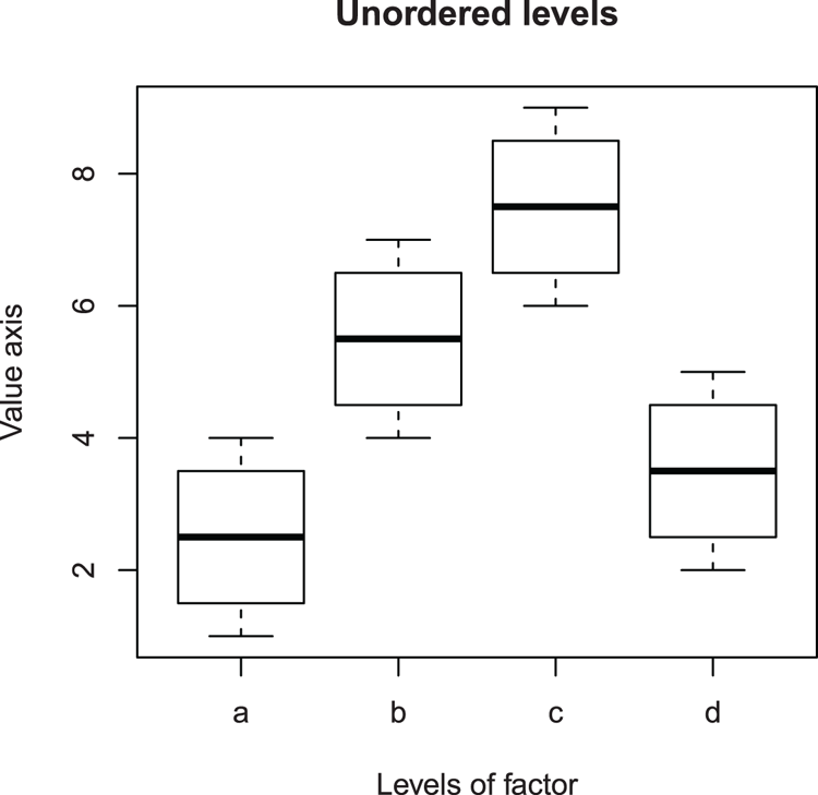
> boxplot(newvec ~ reorder(newfac, newvec, FUN = median)) # Reordered by median

  ## Give the graph some titles
> title(main = "Orderd levels (by median)", xlab = "Levels of factor",
 ylab = "Value axis")
  ## Makes Figure 1-2
Figure 1-2: Boxplot using factor ordered by median (using the reorder command)
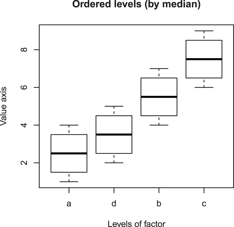
  ## Make frame using data from previous example
  ## vec = Numeric vector, fac = Factor, simple alphabetical labels
> newdf = data.frame(vec = c(1:4, 4:7, 6:9, 2:5),
 fac = gl(n = 4, k = 4, labels = letters[1:4]))

  ## Reorder the factor using the mean
  ## na.rm = TRUE not strictly needed as no NA
> with(newdf, reorder(x = fac, X = vec, FUN = mean, na.rm = TRUE))
 [1] a a a a b b b b c c c c d d d d
attr(,"scores")
  a   b   c   d
2.5 5.5 7.5 3.5
Levels: a d b c
Command Name
row.namesGets or sets row names for data frame objects.
Common Usage
row.names(x)

row.names(x) <- value
Related Commands
Command Parameters
| x | A data frame object. |
| value | The row names to set as some form of character. |
Examples
  ## A simple data frame
> newdf = data.frame(col1 = 1:3, col2 = 4:6)

  ## Examine row names
> row.names(newdf)
[1] "1" "2" "3"

  ## Set row names (using month names)
> row.names(newdf) = month.name[1:3]

> ## View result
> newdf
         col1 col2
January     1    4
February    2    5
March       3    6

  ## Reset names to NULL
> row.names(newdf) = NULL # Produces simple index values
> newdf
  col1 col2
1    1    4
2    2    5
3    3    6
Command Name
rownamesViews or sets row names for matrix and data frame objects.
Common Usage
rownames(x)

rownames(x) <- value
Related Commands
Command Parameters
| x | An R object, usually a data frame or matrix. |
| value | The column names to set as some form of character. |
Examples
  ## Make some objects
> newdf = data.frame(col1 = 1:3, col2 = 4:6)
> newlist = list(item1 = letters[1:5], item2 = 100:110)
> newmat = matrix(1:12, nrow = 3, dimnames = list(letters[1:3], LETTERS[1:4]))

  ## Examine row names
> rownames(newdf)
[1] "1" "2" "3"

> rownames(newlist) # Fails – not a matrix or data frame
NULL

> rownames(newmat)
[1] "a" "b" "c"

  ## Set row names
> rownames(newdf) = LETTERS[1:3] # Use uppercase letters
> rownames(newdf) = c("First", "Second", "Third") # Set explicitly
Command Name
storage.modeThe storage.mode of an object is an attribute related to how it is stored in the R environment. The class, mode, and storage.mode attributes are all related to the type of object. The storage.mode command can get current values or set new ones.
Common Usage
storage.mode(x)

storage.mode(x) <- value
Related Commands
Command Parameters
| x | An R object. |
| value | A character string giving the new storage mode to assign to the object. |
Examples
  ## Make some objects
> newlist = list(Ltrs = letters[1:5], Nmbrs = 100:110)
> newmat = matrix(1:12, nrow = 3, dimnames = list(letters[1:3], LETTERS[1:4]))
> newdf = data.frame(col1 = 1:3, col2 = 4:6)
> newint = 1:10
> newnum = c(1.5, 2.3, 4.7)
> newchar = month.abb[1:6]
> newfac = gl(3,3, labels = c("hi", "mid", "lo"))

  ## Get the storage modes
> storage.mode(newlist)
[1] "list"

> storage.mode(newmat)
[1] "integer"

> storage.mode(newdf)
[1] "list"

> storage.mode(newint)
[1] "integer"

> storage.mode(newnum)
[1] "double"

> storage.mode(newchar)
[1] "character"

> storage.mode(newfac)
[1] "integer"
Command Name
strDisplays the structure of an R object.
Common Usage
str(object)Related Commands
Command Parameters
| object | An R object. |
Examples
  ## Make some objects
> newlist = list(Ltrs = letters[1:5], Nmbrs = 100:110)
> newmat = matrix(1:12, nrow = 3, dimnames = list(letters[1:3], LETTERS[1:4]))
> newdf = data.frame(col1 = 1:3, col2 = 4:6)
> newvec = 1:6

  ## Look at object structure
> str(newdf)
'data.frame': 3 obs. of  2 variables:
$ col1: int  1 2 3
 $ col2: int  4 5 6

> str(newlist)
List of 2
 $ Ltrs : chr [1:5] "a" "b" "c" "d" ...
 $ Nmbrs: int [1:11] 100 101 102 103 104 105 106 107 108 109 ...

> str(newmat)
 int [1:3, 1:4] 1 2 3 4 5 6 7 8 9 10 ...
 - attr(*, "dimnames")=List of 2
  ..$ : chr [1:3] "a" "b" "c"
  ..$ : chr [1:4] "A" "B" "C" "D"

> str(newvec)
 int [1:6] 1 2 3 4 5 6
Command Name
typeofDetermines the type (R internal storage mode) of an object. The command returns a character string giving the type. Usually the typeof command gives the same result as the storage.mode command, but not the mode command.
Common Usage
typeof(x)Related Commands
Command Parameters
| x | An R object. |
Examples
  ## Make some objects
> newlist = list(Ltrs = letters[1:5], Nmbrs = 100:110)
> newmat = matrix(1:12, nrow = 3, dimnames = list(letters[1:3], LETTERS[1:4]))
> newdf = data.frame(col1 = 1:3, col2 = 4:6)
> newint = 1:10
> newnum = c(1.5, 2.3, 4.7)
> newchar = month.abb[1:6]
> newfac = gl(3,3, labels = c("hi", "mid", "lo"))

  ## Get the types
> typeof(newlist)
[1] "list"

> typeof(newmat)
[1] "integer"

> typeof(newdf)
[1] "list"

> typeof(newint)
[1] "integer"

> typeof(newnum)
[1] "double"

> typeof(newchar)
[1] "character"

> typeof(newfac)
[1] "integer"
Command Name
unclassR stores various types of objects and many have a class attribute. This is used by some commands to handle the object in a particular manner. The unclass command returns a copy of the object with the class attribute removed.
Common Usage
unclass(object)Related Commands
Command Parameters
| object | An R object. |
Examples
  ## Make some objects
> newlist = list(Ltrs = letters[1:5], Nmbrs = 100:110)
> newmat = matrix(1:12, nrow = 3, dimnames = list(letters[1:3], LETTERS[1:4]))
> newdf = data.frame(col1 = 1:3, col2 = 4:6)
> newvec = 1:6

  ## Return copy of objects with class attribute removed
> unclass(newlist) # Not much affected
$Ltrs
[1] "a" "b" "c" "d" "e"

$Nmbrs
 [1] 100 101 102 103 104 105 106 107 108 109 110

> unclass(newmat) # Not much affected
  A B C  D
a 1 4 7 10
b 2 5 8 11
c 3 6 9 12

> unclass(newvec) # Not much affected
[1] 1 2 3 4 5 6

> unclass(newdf) # Is affected
$col1
[1] 1 2 3

$col2
[1] 4 5 6

attr(,"row.names")
[1] 1 2 3

  ## Unclass makes data frame act like list
> mydf = unclass(newdf)
> class(mydf)
[1] "list"
Command name
unlistThis command takes a list object and simplifies it to produce a vector object. This can produce a more readable output.
Common usage
unlist(x, use.names = TRUE)Related commands
Command parameters
| x | A list object. |
| use.names = TRUE | By default the names of the list elements are preserved as names in the resulting vector. If use.names = FALSE the resulting vector is unnamed. |
Examples
  ## Create three vectors
> mow = c(12, 15, 17, 11, 15)
> unmow = c(8, 9, 7, 9)
> chars = LETTERS[1:5]

  ## Make lists
> l1 = list(mow = mow, unmow = unmow) # All elements numeric
> l2 = list(mow = mow, unmow = unmow, chars = chars) # Mix of numeric and text

> unlist(l1)
  mow1   mow2   mow3   mow4   mow5 unmow1 unmow2 unmow3 unmow4
    12     15     17     11     15      8      9      7      9

> unlist(l1, use.names = FALSE)
[1] 12 15 17 11 15  8  9  7  9

> unlist(l2)
  mow1   mow2   mow3   mow4   mow5 unmow1 unmow2 unmow3 unmow4 chars1 chars2
  "12"   "15"   "17"   "11"   "15"    "8"    "9"    "7"    "9"    "A"    "B"
chars3 chars4 chars5
   "C"    "D"    "E"
Command Name
variable.namesShows the variable names for fitted models or the column names for data frames and matrix objects.
Common Usage
variable.names(object)Related Commands
Command Parameters
| object | An R object, usually a fitted model result but can be a matrix or data frame. |
Examples
  ## Make some objects:
  ## A matrix
> newmat = matrix(1:12, nrow = 3, dimnames = list(letters[1:3], LETTERS[1:4]))

  ## A data frame
> newdf = data.frame(col1 = 1:3, col2 = 4:6, row.names = letters[1:3])

  ## A linear model result
> newlm = lm(col2 ~ col1, data = newdf)

> ## Examine variable names
> variable.names(newmat)
[1] "A" "B" "C" "D"

> variable.names(newdf)
[1] "col1" "col2"

> variable.names(newlm)
[1] "(Intercept)" "col1"
Selecting and Sampling Data
Data objects exist in a variety of forms, and often you will want to extract only a part of an existing object. This part may be a single column of a data frame or an item from a list. You may also want to extract values that correspond to some particular value.
Command Name
[]The square brackets enable you to select/extract parts of an object. For vector objects that have a single dimension, a single value is required. For matrix and data frame objects that are two-dimensional, two values (row, column) are needed.
Common Usage
x[i]
x[i, j, ...]
Related Commands
Command Parameters
| x | An R object. |
| i, j | Indices used to specify elements. |
| ... | Other commands (including indices). |
Examples
  ## Make some objects
> newlist = list(Ltrs = letters[1:5], Nmbrs = 100:110)
> newdf = data.frame(col1 = 1:3, col2 = 4:6)
> newnum = c(1.5, 2.3, 4.7)
> newarr = array(1:12, dim = c(2, 3, 2),
 dimnames = list(letters[1:2], LETTERS[1:3], c("One", "Two")))

  ## Extract some elements of objects
> newlist[2] # 2nd element of list
$Nmbrs
 [1] 100 101 102 103 104 105 106 107 108 109 110


> newdf[2:3, 1:2] # rows 2-3 and columns 1-2 of data frame
  col1 col2
2    2    5
3    3    6

> newdf[1:2,] # rows 1-2 and all columns of data frame
  col1 col2
1    1    4
2    2    5

> newnum[-2] # all except 2nd item of vector
[1] 1.5 4.7

> newarr[, c(1, 3), 2] # all rows and columns 1&3 for 2nd part of array
  A  C
a 7 11
b 8 12

  ## Replace or add to object
> newnum[4] = 9.9 # Add new item to end
> newnum[2] = 7.7 # Replace 2nd item
> newnum # View modified vector
[1] 1.5 7.7 4.7 9.9

> newdf[, 3] = 7:9 # Add unnamed column to data frame
> newdf[, "col3"] = 10:12 # Add named column to data frame
> newdf # View modifications
  col1 col2 V3 col3
1    1    4  7   10
2    2    5  8   11
3    3    6  9   12
Command Name
$Objects can have several elements; for example, columns of a data frame or list items. The $ enables you to select elements within an object and either extract them or alter the values. You can also use the $ to add an element to an existing object. The $ can only be used for list and data frame objects (that is, ones with a names attribute).
Common Usage
x$name
x$name <- value
Related Commands
Command Parameters
| x | An R object, usually a list or data frame. |
| name | A character string or name. |
| value | A value to assign to the selected element. |
Examples
  ## Make some objects
> newlist = list(Ltrs = letters[1:5], Nmbrs = 100:110) # List
> newdf = data.frame(col1 = 1:3, col2 = 4:6) # Data frame
> newlm = lm(col1 ~ col2, data = newdf) # Linear model result

  ## Check names
> names(newlist)
[1] "Ltrs"  "Nmbrs"

> names(newdf)
[1] "col1" "col2"

> names(newlm) # Result object is a form of list
[1] "coefficients"  "residuals"     "effects"       "rank"
[5] "fitted.values" "assign"        "qr"            "df.residual"
[9] "xlevels"       "call"          "terms"         "model"

  ## View named elements
> newlist$Ltrs
[1] "a" "b" "c" "d" "e"

> newdf$col2
[1] 4 5 6

> newlm$coefficients
(Intercept)        col2
         -3           1

  ## Add elements
> newdf$col3 = 7:9 # Add new column to data frame
> newdf # View result
  col1 col2 col3
1    1    4    7
2    2    5    8
3    3    6    9

> newlist$Mnth = month.abb[1:3] # Add new item to list
> newlist # View result
$Ltrs
[1] "a" "b" "c" "d" "e"

$Nmbrs
 [1] 100 101 102 103 104 105 106 107 108 109 110

$Mnth
[1] "Jan" "Feb" "Mar"

  ## Replace elements
> newdf$col2 = c(100, 101, 102) # Replace whole column
> newdf # View result
  col1 col2 col3
1    1  100    7
2    2  101    8
3    3  102    9

> newlist$Ltrs[3] = "z" # Replace single item using []
> newlist # View result
$Ltrs
[1] "a" "b" "z" "d" "e"

$Nmbrs
 [1] 100 101 102 103 104 105 106 107 108 109 110

$Mnth
[1] "Jan" "Feb" "Mar"
Command Name
droplevels This command will drop unused levels of factors from the object specified. Usually this will be a data frame that contains multiple columns, including factors. The subset command is used to create a subset of a dataset but this does not drop the levels from the original. The unused levels will thus appear in graphs and tables, for example (albeit with zero count, see the following examples).
Common Usage
droplevels(x, except, ...)Related Commands
Command Parameters
| x | An object from which unused levels are to be dropped. Usually this is a data frame that contains columns of factors but you can also specify a single factor object. |
| except | Columns for which the levels should not be dropped. These are specified as a vector of column numbers or the names (in quotes) of the variables. |
| ... | Other arguments from other methods can be used if appropriate. |
Examples
  ## Use InsectSprays data from R datasets
> data(InsectSprays) # Make sure data is ready

  ## Look at InsectSprays dataset
> str(InsectSprays) # View data structure
'data.frame': 72 obs. of  2 variables:
 $ count: num  10 7 20 14 14 12 10 23 17 20 ...
 $ spray: Factor w/ 6 levels "A","B","C","D",..: 1 1 1 1 1 1 1 1 1 1 ...

> levels(InsectSprays$spray) # View levels of spray factor
[1] "A" "B" "C" "D" "E" "F"
> table(InsectSprays$spray) # View levels of spray as table of replicates

 A  B  C  D  E  F
12 12 12 12 12 12

  ## Make a subset without spray "C"
> ISs = subset(InsectSprays, spray != "C") # Subset and lose spray "C"

> levels(ISs$spray) # View levels, spray "C" is sill present
[1] "A" "B" "C" "D" "E" "F"
> table(ISs$spray) # View as table, spray "C" has no data

 A  B  C  D  E  F
12 12  0 12 12 12

  ## Drop the unused levels
> ISd = droplevels(ISs) # Drop unused levels
> table(ISd$spray) # Spray "C" now not present

 A  B  D  E  F
12 12 12 12 12
Command Name
resampleTakes random samples and permutations. This is a custom function that you must create in order to use. It overcomes a computational quirk in the sample command where an unexpected result occurs when a conditional sample is used (see the following examples).
Common Usage
Create the custom function like so:
resample <- function(x, ...) x[sample(length(x), ...)]Use the new function exactly like the sample command:
resample(x, size, replace = FALSE)Related Commands
Command Parameters
| x | A vector of values. |
| size | The number of items to choose. |
| replace = FALSE | If replace = TRUE, items can be selected more than once (that is, re-placed). |
Examples
  ## Make a vector
> newvec = 1:10

  ## Conditional selection
  ## sample() command has a quirk!
> sample(newvec[newvec > 8]) # This is fine
[1] 10  9

> sample(newvec[newvec > 9]) # This is wrong!
 [1]  3  5  4 10  2  7  8  1  9  6

> sample(newvec[newvec > 10]) # This is fine
integer(0)

  ## Create custom function
> resample <- function(x, ...) x[sample(length(x), ...)]

  ## Try conditional selection again
> resample(newvec[newvec > 8]) # Fine, same as before
[1]  9 10

> resample(newvec[newvec > 9]) # This is now correct
[1] 10

> resample(newvec[newvec > 10]) # Fine, same as before
integer(0)
Command Name
sampleTakes random samples and permutations. The sample command takes a sample of specified size from a specified object using replacement or not (as you specify). Due to the computational process used, some results can be unexpected when conditional sampling is used.
Common Usage
sample(x, size, replace = FALSE)Related Commands
Command Parameters
| x | A vector of values. |
| size | The number of items to choose. |
| replace = FALSE | If replace = TRUE, items can be selected more than once (that is, re-placed). |
Examples
  ## Make some vector samples
> newnum = 1:10
> newchar = month.abb[1:12]

  ## Sampling: effects of replacement
> set.seed(4) # Set random number seed
> sample(newchar, size = 4, replace = TRUE) # With replacement
[1] "Aug" "Jan" "Apr" "Apr"

> set.seed(4) # Set random number seed
> sample(newchar, size = 4) # Without replacement (the default)
[1] "Aug" "Jan" "Mar" "Oct"

  ## Sample: matching an expression
> set.seed(3) # Set random number seed
> sample(newnum[newnum > 5], size = 2) # Get 2 items larger than 5
[1] 6 9

> set.seed(3) # Set random number seed
> sample(newnum[newnum > 5]) # Get all items larger than 5
[1]  6  9  7 10  8

> set.seed(3) # Set random number seed
> sample(newnum  > 5) # Logical result
 [1] FALSE  TRUE FALSE FALSE  TRUE  TRUE FALSE FALSE  TRUE  TRUE

> set.seed(3) # Set random number seed
> sample(newnum == 5) # Logical result, N.B. double ==
 [1] FALSE FALSE FALSE FALSE FALSE FALSE FALSE  TRUE FALSE FALSE
Command Name
subsetThis command extracts subsets of data objects (vectors, data frames, and matrix objects), which meet certain conditions. Note that subset is used as a parameter within many commands and can use a special syntax (see the following examples).
Common Usage
subset(x, subset, select)
command(subset = group %in% c("a", "b", ...))
Related Commands
Command Parameters
| x | An object. Can be a vector, matrix, or, more commonly, a data frame. |
| subset | An expression indicating which items to keep. When used as a parameter the syntax can be of the form subset = group %in% c("a", "b", ...) for example. |
| select | An expression indicating which columns to select from a data frame. |
Examples
  ## Make a data frame: val = numeric, fac = 4-level factor
> newdf = data.frame(val = 1:12, fac = gl(n = 4, k = 3, labels = LETTERS[1:4]))

  ## Generate some subsets
> subset(newdf, subset = val > 5) # All columns shown as default
   val fac
6    6   B
7    7   C
8    8   C
9    9   C
10  10   D
11  11   D
12  12   D

> subset(newdf, subset = val > 5, select = c(fac, val)) # Columns in new order
   fac val
6    B   6
7    C   7
8    C   8
9    C   9
10   D  10
11   D  11
12   D  12

> subset(newdf, subset = fac == "C", select = c(fac, val))
  fac val
7   C   7
8   C   8
9   C   9

> subset(newdf, subset = val > 5 & fac == "D") # Two subsets 1 AND 2
   val fac
10  10   D
11  11   D
12  12   D

  ## Alternative syntax, often encountered when subset used as a parameter
> subset(newdf, subset = fac %in% "D")
   val fac
10  10   D
11  11   D
12  12   D
Command Name
whichReturns an index value for an expression. In other words, you can get an index value for the position of items in a vector or array that match certain conditions.
Common Usage
which(x. array.ind = FALSE)Related Commands
Command Parameters
| x | An R object, usually a vector, matrix, or array. |
| array.ind = FALSE | If array.ind = TRUE, the result is shown as an array. |
Examples
  ## Make objects
> newnum = 10:1 # Descending values
> newchar = month.abb[1:12] # Characters (month names)
> newarr = array(1:12, dim = c(2, 3, 2),
 dimnames = list(letters[1:2], LETTERS[1:3], c("One", "Two"))) # A 3D array

  ## Get index values
> which(newchar == "Apr") # How far along the sequence is "Apr"?
[1] 4
> newchar
 [1] "Jan" "Feb" "Mar" "Apr" "May" "Jun" "Jul" "Aug" "Sep" "Oct" "Nov" "Dec"

> which(newnum == 5) # Which item(s) equal 5?
[1] 6
> newnum
 [1] 10  9  8  7  6  5  4  3  2  1

> which(newnum > 5) # Which items are greater than 5?
[1] 1 2 3 4 5

> which(newarr > 5) # Which items in array are greater than 5?
[1]  6  7  8  9 10 11 12

> which(newarr > 5, arr.ind = TRUE) # Shows result as an array
  dim1 dim2 dim3
b    2    3    1
a    1    1    2
b    2    1    2
a    1    2    2
b    2    2    2
a    1    3    2
b    2    3    2
Command Name
withAllows an object to be temporarily placed in the search list. The result is that named components of the object are available for the duration of the command.
Sorting and Rearranging Data
Data within an object is usually unsorted; that is, it is arranged in the order in which the values were entered. For this reason, it can be useful to have an index for the order in which the items lie. It can also be useful to rearrange data into a new order.
Command Name
orderReturns the order in which items of a vector are arranged. In other words, you get an index value for the order of items. The command can use additional vectors to act as tie-breakers. This command can help to rearrange data frames and matrix objects by creating an index that can be used with the [] to specify a new row (or column) arrangement.
Common Usage
order(..., na.last = TRUE, decreasing = FALSE)Related Commands
Command Parameters
| ... | R objects (vectors); all must be of the same length. The first named item is ordered and subsequent items are used to resolve ties. |
| na.last = TRUE | Controls treatment of NA items. If TRUE, NA items are placed at the end, if FALSE they are placed at the beginning, and if NA they are omitted. |
| decreasing = FALSE | If decreasing = TRUE, the items are ordered in descending fashion. |
Examples
  ## Make objects
> newvec = c(3, 4, NA, 7, 1, 6, 5, 5, 2) # Vector containing NA
> tv1 = 1:9 # Vector of ascending values
> tv2 = 9:1 # Vector of descending values

  ## Get index for order of items
> order(newvec) # Default, ascending with NA last
[1] 5 9 1 2 7 8 6 4 3

> order(newvec, na.last = FALSE) # Ascending with NA first
[1] 3 5 9 1 2 7 8 6 4

> order(newvec, na.last = NA) # Ascending NA omitted
[1] 5 9 1 2 7 8 6 4

> order(newvec, na.last = NA, decreasing = TRUE) # Decreasing with NA omitted
[1] 4 6 7 8 2 1 9 5

  ## Effects of using a tie-breaker
> tv1 ; tv2 # view tie-breaker vectors
[1] 1 2 3 4 5 6 7 8 9
[1] 9 8 7 6 5 4 3 2 1

> order(newvec, tv1) # Same order as before (7, 8)
[1] 5 9 1 2 7 8 6 4 3

> order(newvec, tv2) # Different order (8, 7)
[1] 5 9 1 2 8 7 6 4 3
Command Name
rankGives the ranks of the values in a vector. The default method produces values that are used in a wide range on non-parametric statistical tests.
Common Usage
rank(x, na.last = TRUE, ties.method = "average")Related Commands
Command Parameters
| x | A vector of values. |
| na.last = TRUE | Sets how NA items are handled. If na.last = TRUE, NA items are put last; if FALSE they are put first; and if na.last = NA they are omitted. |
| ties.method = "average" | Sets the method to determine how to deal with tied values. The default, "average", uses the mean. Alternatives are "first", "random", "max", and "min". The method name can be abbreviated (but must be in quotes). |
Examples
  ## Make a vector
> newvec = c(3, 4, NA, 7, 1, 6, 5, 5, 2) # Vector containing NA

  ## Rank vector
> rank(newvec) # Using default (NA placed last, "average" method)
[1] 3.0 4.0 9.0 8.0 1.0 7.0 5.5 5.5 2.0

> rank(newvec, na.last = NA, ties.method = "average") # Remove NA
[1] 3.0 4.0 8.0 1.0 7.0 5.5 5.5 2.0

> rank(newvec, na.last = FALSE, ties.method = "max") # NA 1st, "max" method
[1] 4 5 1 9 2 8 7 7 3

> rank(newvec, na.last = FALSE, ties.method = "min") # NA 1st, "min" method
[1] 4 5 1 9 2 8 6 6 3
Command Name
sortRearranges data into a new order.
Common Usage
sort(x, decreasing = FALSE, na.last = NA)Related Commands
Command Parameters
| x | A vector. |
| decreasing = FALSE | If set to TRUE, the vector is sorted in descending order. |
| na.last = NA | Sets how to deal with NA items. If na.last = NA (the default), NA items are omitted. If set to TRUE, they are placed last and if FALSE, they are placed first. |
Examples
  ## Make a vector
> newvec = c(3, 4, NA, 7, 1, 6, 5, 5, 2) # Vector containing NA

> ## Sort vector
> sort(newvec) # The defaults, ascending order with NA omitted
[1] 1 2 3 4 5 5 6 7

> sort(newvec, na.last = TRUE) # Place NA last
[1]  1  2  3  4  5  5  6  7 NA

> sort(newvec, na.last = FALSE, decreasing = TRUE) # NA 1st, descending order
[1] NA  7  6  5  5  4  3  2  1
Command Name
whichReturns an index value for an expression. In other words, you can get an index value for the position of items in a vector or array that match certain conditions.
Summarizing Data
The more complicated and large an object is (large meaning lots of values), the more important it is to summarize the object in a more compact and meaningful manner.
What’s In This Topic:
- Averages and statistics for simple objects (vectors)
- Summarizing complicated objects (e.g., data frames or lists)
- Summary statistics for table and table-like objects
- Contingency tables
- Cross tabulation
Summary Statistics
It is important to be able to summarize data in a compact and meaningful manner. R provides various commands to carry out summary statistics as well as methods for dealing with complicated objects, such as data frames, with columns containing numerical and factor data.
Command Name
addmarginsCarries out a summary command on a table, array, or matrix object. You can specify the command and which margins to use.
Command Name
aggregateComputes summary statistics on complicated objects based on grouping variables. The command accepts input in two different ways (see the following common usage). The formula input is a convenient way to carry out summaries on data frames.
Common Usage
aggregate(x, by, FUN, ...)

aggregate(formula, data, FUN, ..., subset, na.action = na.omit)
Related Commands
Command Parameters
| x | An R object. |
| by | A list of grouping elements, each the same length as the variable(s) in x. |
| FUN | The function to compute as a summary statistic. |
| ... | Other relevant parameters; e.g., na.omit = TRUE. |
| formula | A formula specifying the variable to summarize on the left and the grouping variables on the right; e.g., y ~ x + z. |
| subset | An optional vector specifying a subset to use. |
| na.action = na.omit | For the formula method, NA items are omitted by default. |
Examples
  ## Make some objects
> vec = 1:16 # Simple numeric vector
> fac1 = gl(n = 4, k = 4, labels = LETTERS[1:4]) # Factor 4 levels
> fac2 = gl(n = 2, k = 8, labels = c("First", "Second")) # Factor 2 levels
> newdf = data.frame(resp = vec, pr1 = fac1, pr2 = fac2) # Data frame

  ## Summarize
> aggregate(vec, by = list(fac1), FUN = max) # For one grouping
  Group.1  x
1       A  4
2       B  8
3       C 12
4       D 16

> aggregate(vec, by = list(fac1, fac2), FUN = median) # 2 grouping variables
  Group.1 Group.2    x
1       A   First  2.5
2       B   First  6.5
3       C  Second 10.5
4       D  Second 14.5

> aggregate(resp ~ pr1 + pr2, data = newdf, FUN = sum) # Formula method
  pr1    pr2 resp
1   A  First   10
2   B  First   26
3   C Second   42
4   D Second   58
Command Name
applyApplies a function over the margins of an array or matrix.
Common Usage
apply(X, MARGIN, FUN, ...)Related Commands
Command Parameters
| X | An array or matrix. |
| MARGIN | The margin over which the summary function is to be applied; e.g., MARGIN = 1 summarizes rows, 2 summarizes columns. |
| FUN | The function to apply to the data. |
| ... | Other relevant parameters as accepted by FUN; e.g., na.rm = TRUE. |
Examples
  ## Make objects
> newarr = array(1:12, dim = c(2, 3, 2),
 dimnames = list(letters[1:2], LETTERS[1:3], c("One", "Two"))) # A 3D array
> newmat = matrix(1:24, nrow = 3, dimnames = list(letters[1:3], LETTERS[1:8]))
> newmat[5] = NA # Make one element a missing value, NA

  ## Summarize
> apply(newarr, MARGIN = 1, FUN = sum) # Sum for dimension 1 of array
 a  b
36 42

> apply(newarr, MARGIN = c(2, 3), FUN = sum) # Sum for 2 dimensions of array
  One Two
A   3  15
B   7  19
C  11  23

> apply(newmat, MARGIN = 2, FUN = median) # Median for columns of matrix
 A  B  C  D  E  F  G  H
 2 NA  8 11 14 17 20 23

> apply(newmat, MARGIN = 2, FUN = median, na.rm = TRUE) # Omit NA items
 A  B  C  D  E  F  G  H
 2  5  8 11 14 17 20 23
Command Name
colMeans
colSums
rowMeans
rowSums
Simple column (or row) sums or means for array or matrix objects. These are equivalent to the apply command with FUN = mean or FUN = sum, but are computationally more efficient. Compare to the rowsum command, which uses a grouping variable.
Common Usage
colMeans(x, na.rm = FALSE, dims = 1)
colSums(x, na.rm = FALSE, dims = 1)
rowMeans(x, na.rm = FALSE, dims = 1)
rowSums(x, na.rm = FALSE, dims = 1)
Related Commands
Command Parameters
| x | An array of two or more dimensions or a data frame. |
| na.rm = FALSE | If na.rm = TRUE, NA items are omitted. |
| dims = 1 | An integer value stating how many dimensions to calculate over. This must be at least one less than the total number of dimensions. The row and col commands treat this value differently (see the following examples). |
Examples
  ## Make objects
> newarr = array(1:12, dim = c(2, 3, 2),
 dimnames = list(letters[1:2], LETTERS[1:3], c("One", "Two"))) # A 3D array
> newmat = matrix(1:24, nrow = 3, dimnames = list(letters[1:3], LETTERS[1:8]))
> newmat[5] = NA # Make one element a missing value, NA

  ## Summarize
> colMeans(newmat) # Default, NA items not omitted
 A  B  C  D  E  F  G  H
 2 NA  8 11 14 17 20 23

> colMeans(newmat, na.rm = TRUE) # Omit NA item
 A  B  C  D  E  F  G  H
 2  5  8 11 14 17 20 23

> colSums(newarr, dims = 1) # For cols one dimension at a time
  One Two
A   3  15
B   7  19
C  11  23

> colSums(newarr, dims = 2) # For cols dimensions combined
One Two
 21  57

> rowSums(newarr, dims = 1) # For rows dimensions combined
 a  b
36 42

> rowSums(newarr, dims = 2) # For rows one dimension at a time
   A  B  C
a  8 12 16
b 10 14 18
Command Name
colSumsSimple column sums for array or matrix objects.
Command Name
cummax
cummin
cumprod
cumsum
These commands provide functions for carrying out cumulative operations. The commands return values for cumulative maxima, minima, product, and sum. If used with the seq_along command, they can provide cumulative values for other functions.
Command Name
fivenumThis command produces Tukey’s five-number summary for the input data. The values returned are minimum, lower-hinge, median, upper-hinge, and maximum.
Command Name
IQRCalculates the inter-quartile range.
Command Name
lapplyApplies a function to elements of a list. The result is also a list.
Common Usage
lapply(X, FUN, ...)Related Commands
Command Parameters
| X | A list object. |
| FUN | The function to apply to each element of the list. |
| ... | Other parameters relevant to the FUN applied; e.g., na.rm = TRUE. |
Examples
  ## Make a list
> newlist = list(num = 1:10, vec = c(2:5, 4:5, 6:8, NA, 9, 12, 17), lg = log(1:5))

  ## Summarize
> lapply(newlist, FUN = mean, na.rm = TRUE)
$num
[1] 5.5

$vec
[1] 6.833333

$lg
[1] 0.9574983
Command Name
lengthDetermines how many elements are in an object. The command can get or set the number of elements.
Common Usage
length(x)

length(x) <- value
Related Commands
Command Parameters
| x | An R object, usually a vector, list, or factor, but other objects may be specified. |
| value | The value to set for the length of the specified object. |
Examples
  ## Make some objects
> newmat = matrix(1:12, nrow = 3) # A matrix
> newlist = list(num = 1:10, ltr = letters[1:6], vec = c(3, 4, NA, 7)) # A list
> newdf = data.frame(col1 = 1:3, col2 = 4:6, col3 = 5:3) # A data frame
> newfac = gl(n = 4, k = 3) # A factor
> newchar = month.abb[1:12] # Character vector
> newnum = 4:12 # Numerical vector

  ## Get Lengths
> length(newmat) # The number of items in the matrix
[1] 12

> length(newlist) # How many elements
[1] 3

> length(newdf) # Number of columns
[1] 3

> length(newfac) # Number of items (not number of different factors)
[1] 12

> length(newchar) # How many items
[1] 12

> length(newnum) # How many items
[1] 9

 ## Alter lengths
> length(newnum) = 12
> newnum # Object is padded with NA
 [1]  4  5  6  7  8  9 10 11 12 NA NA NA

> length(newnum) = 6
> newnum # Object is truncated
[1] 4 5 6 7 8 9
Command Name
madThis command calculates the median absolute deviation for a numeric vector. It also adjusts (by default) by a factor for asymptotically normal consistency.
Command Name
margin.tableProduces sum values for margins of a contingency table, array, or matrix.
Command Name
meanCalculates the mean value for the specified data.
Command Name
medianThis command calculates the median value for an object.
Command Name
prop.tableThis command expresses table entries as a fraction of the marginal total.
Command Name
quantileReturns quantiles for a sample corresponding to given probabilities. The default settings produce five quartile values.
Command Name
rangeGives the range for a given sample; that is, a vector containing the minimum and maximum values.
Command Name
rowMeansSimple row means for array or matrix objects.
Command Name
rowsumThis command sums columns of a matrix or data frame based on a grouping variable. The column sums are computed across rows of a matrix for each level of a grouping variable. Contrast this to the colSums command, which produces a simple sum of each column.
Common Usage
rowsum(x, group, reorder = TRUE, na.rm = TRUE)Related Commands
Command Parameters
| x | An R object; usually a data frame, matrix, table, or array. |
| reorder = TRUE | If reorder = FALSE, the result is in the order in which the groups were encountered. |
| na.rm = FALSE | If na.rm = TRUE, NA items are omitted. |
Examples
  ## Make objects
> newdf = data.frame(col1 = 1:6, col2 = 8:3, col3 = 6:1) # Numeric 3 columns
> newchar = c("C", "C", "B", "B", "A", "A") # Grouping vector
> newdf # View original data frame
  col1 col2 col3
1    1    8    6
2    2    7    5
3    3    6    4
4    4    5    3
5    5    4    2
6    6    3    1

  ## Row sums by group
> rowsum(newdf, group = newchar) # Groups are re-ordered
  col1 col2 col3
A   11    7    3
B    7   11    7
C    3   15   11

> rowsum(newdf, group = newchar, reorder = FALSE) # Keep original group order
  col1 col2 col3
C    3   15   11
B    7   11    7
A   11    7    3
Command Name
rowSumsSimple row sums for array or matrix objects.
Command Name
sapplyApplies a function to elements of a list (or a vector). The result is a matrix.
Common Usage
sapply(X, FUN, ...,)Related Commands
Command Parameters
| X | A list or vector object. |
| FUN | The function to apply to the elements of the object. |
| ... | Other parameters relevant to the FUN used. |
Examples
  ## Make a list
> newlist = list(num = 1:10, vec = c(2:5, 4:5, 6:8, NA, 9, 12, 17), lg = log(1:5))

  ## Summarize
> sapply(newlist, FUN = mean, na.rm = TRUE)
      num       vec        lg
5.5000000 6.8333333 0.9574983
Command Name
sdCalculates standard deviation for vector, matrix, and data frame objects. If the data is a matrix or data frame, the standard deviation is calculated for each column.
Command Name
sumThis command returns the sum of the values present.
Command Name
summarySummarizes an object. This command is very general and the result depends on the class of the object being examined. Some results objects will have a special class and possibly a dedicated summary routine to display them.
Common Usage
summary(object, maxsum = 7, digits = max(3, getOption("digits")-3)Related Commands
Command Parameters
| object | An R object. |
| maxsum = 7 | An integer value indicating the maximum number of levels of a factor to show. For a data frame this defaults to 7, but for a factor object the default is 100. |
| digits = | The number of digits to display for numeric variables. |
Examples
  ## Make objects
> newnum = c(2:5, 4:5, 6:8, 9, NA, 17) # Numeric vector
> newfac = factor(c(rep("A", 3), rep("B", 3), rep("C", 3), rep("D", 2)))
> newdf = data.frame(response = na.omit(newnum), predictor = newfac)
> newchar = month.abb[1:12]
> newlist = list(Ltr = letters[1:10], Nmbr = 1:12)

  ## Summary
> summary(newnum)
   Min. 1st Qu.  Median    Mean 3rd Qu.    Max.    NA's
  2.000   4.000   5.000   6.364   7.500  17.000   1.000

> summary(newfac)
A B C D
3 3 3 2

> summary(newdf)
    response      predictor
 Min.   : 2.000   A:3
 1st Qu.: 4.000   B:3
 Median : 5.000   C:3
 Mean   : 6.364   D:2
 3rd Qu.: 7.500
 Max.   :17.000

> summary(newchar)
   Length     Class      Mode
       12 character character

> summary(newlist)
     Length Class  Mode
Ltr  10     -none- character
Nmbr 12     -none- numeric
Command Name
sweepThis command examines an array object and uses a second array with a mathematical operator to sweep out a summary statistic. The result is a new array. The command is particularly useful for comparing items in an array to some other value.
Common Usage
sweep(x, MARGIN, STATS, FUN = "-", ...)Related Commands
Command Parameters
| x | An R object; usually an array, table or matrix. |
| MARGIN | The margin of the array that corresponds to the STATS being swept out. For a matrix, 1 is the rows and 2 is the columns; c(1, 2) gives both. |
| STATS | The summary statistic that is to be swept out. |
| FUN | The function used to carry out the sweep; this is applied like so: x FUN STATS. |
| ... | Optional parameters that may be required by FUN. |
Examples
  ## Make matrix (3 row x 4 col)
> set.seed(5) # Set seed for random numbers
> matdat = round(runif(24, 1, 25)) # Make 24 random values btwn 1 and 25
> newmat = matrix(matdat, nrow = 3,
 dimnames = list(letters[1:3], LETTERS[1:8])) # Make matrix
> newmat # The final matrix
   A  B  C  D  E  F  G  H
a  6  8 14  4  9  6 14 18
b 17  4 20  8 14 10 21  6
c 23 18 24 13  7 22 22  6

  ## Array summaries
  ## Get medians for columns
> matmed = apply(newmat, MARGIN = 2, FUN = median)
> matmed # View the result (a matrix of column medians)
 A  B  C  D  E  F  G  H
17  8 20  8  9 10 21  6

  ## Subtract col medians from original matrix
> sweep(newmat, MARGIN = 2, FUN = "-", STATS = matmed)
    A  B  C  D  E  F  G  H
a -11  0 -6 -4  0 -4 -7 12
b   0 -4  0  0  5  0  0  0
c   6 10  4  5 -2 12  1  0

  ## Multiply each element by itself (same as newmat^2)
> sweep(newmat, MARGIN = c(1,2), FUN = "*", STATS = newmat)
    A   B   C   D   E   F   G   H
a  36  64 196  16  81  36 196 324
b 289  16 400  64 196 100 441  36
c 529 324 576 169  49 484 484  36
Command Name
tapplyThis command enables you to apply a summary function to a vector based on the levels of another vector. You can also use it to make one column (or several) of a data frame a grouping variable to summarize another column.
Common Usage
tapply(X, INDEX, FUN = NULL, ...)Related Commands
Command Parameters
| X | An R object; usually a vector. |
| INDEX | A list of factors, each the same length as X, which act as grouping levels for the function applied in FUN. |
| FUN | The function to be applied; if NULL is used, the result is a simple index. |
| ... | Additional parameters that are relevant to the FUN applied. |
Examples
  ## Make objects
> newnum = c(2:5, 4:5, 6:8, 9, 17) # Numeric vector
> fac1 = factor(c(rep("A", 3), rep("B", 3), rep("C", 3), rep("D", 2))) # Factor
> fac2 = gl(n = 2, k = 1, length = 11, labels = month.abb[1:2]) # Factor
> newdf = data.frame(response = newnum, pred1 = fac1, pred2 = fac2)

  ## Use tapply to summarize by group/level
> tapply(newnum, INDEX = fac1, FUN = NULL) # Gives index
 [1] 1 1 1 2 2 2 3 3 3 4 4

> tapply(newnum, INDEX = fac1, FUN = sum) # Sum for each level of INDEX
 A  B  C  D
 9 14 21 26

> tapply(newnum, INDEX = list(fac1, fac2), FUN = median) # Use 2 INDEX vars
  Jan Feb
A   3   3
B   4   5
C   7   7
D  17   9

  ## Use on a data frame
> with(newdf, tapply(response, INDEX = pred1, FUN = median))
 A  B  C  D
 3  5  7 13
Command name
varThis command calculates the variance of numeric vectors.
Summary Tables
One way to summarize data is to create a contingency table, which shows the frequency of observations at each combination of levels of the variables. R has a range of commands related to the creation and examination of tables; these commands carry out tasks such as making contingency tables, applying summary commands on rows or columns, and cross tabulating.
Command Name
addmarginsCarries out a summary command on a table, array, or matrix object. You can specify the command and which margins to use.
Common Usage
addmargins(A, margin = seq_along(dim(A)), FUN = sum, quiet = FALSE)Related Commands
Command Parameters
| A | An array, table, or matrix object. |
| margin = | The margin to use; the default uses all the dimensions of the object. The result is placed in the margin specified, so margin = 1 produces a row of results, but doesn’t give the results of the row (see the following examples). |
| FUN = sum | The function to use for the summary. The default produces the sum. |
| quiet = FALSE | If several margins are specified explicitly, the command produces a message showing the order in which they were processed. You can suppress the message using quiet = TRUE. |
Examples
  ## Make a matrix
> set.seed(5) # Set random number seed
> matdat = round(runif(n = 24, min = 0, max = 10), 0) # Make 24 random numbers
  ## Now make the matrix (3 rows x 8 columns)
> newmat = matrix(matdat, nrow = 3,
 dimnames = list(letters[1:3], LETTERS[1:8]))

  ## Default: sums for rows, columns and all
> addmargins(newmat)
     A  B  C D  E  F  G  H Sum
a    2  3  5 1  3  2  6  7  29
b    7  1  8 3  6  4  8  2  39
c    9  7 10 5  3  9  9  2  54
Sum 18 11 23 9 12 15 23 11 122

  ## A row of median values (margin = 1)
> addmargins(newmat, margin = 1, FUN = median)
       A B  C D E F G H
a      2 3  5 1 3 2 6 7
b      7 1  8 3 6 4 8 2
c      9 7 10 5 3 9 9 2
median 7 3  8 3 3 4 8 2

  ## A column of Std deviations (margin = 2)
> addmargins(newmat, margin = 2, FUN = sd)
  A B  C D E F G H       sd
a 2 3  5 1 3 2 6 7 2.133910
b 7 1  8 3 6 4 8 2 2.748376
c 9 7 10 5 3 9 9 2 3.058945

  ## Two different functions (one for each margin)
> addmargins(newmat, FUN = list(SUM = sum, Std.Dev. = sd))
Margins computed over dimensions
in the following order:
1:
2:
     A  B  C D  E  F  G  H Std.Dev.
a    2  3  5 1  3  2  6  7 2.133910
b    7  1  8 3  6  4  8  2 2.748376
c    9  7 10 5  3  9  9  2 3.058945
SUM 18 11 23 9 12 15 23 11 5.522681
Command Name
ftableCreates contingency tables using cross-classifying factors to show the frequency of observations at each combination of variables. If a contingency table is created using multiple cross-classifying (grouping) variables, the result is an array with multiple dimensions. The ftable command creates “flat” tables, which are simpler. These tables have a class attribute "ftable".
Common Usage
ftable(..., row.vars = NULL, col.vars = NULL)Related Commands
Command Parameters
| ... | R objects to be tabulated. These can be one or more vectors or a factor, matrix, array, or data frame. |
| row.vars = NULL | If the object has named items (e.g., columns of a data frame), the names or column numbers can be specified as the row items in the final flat table. Otherwise, the order in which the items are specified in ... determines the final outcome. |
| col.vars = NULL | If the object has named items (e.g., columns of a data frame), the names or column numbers can be specified as the column items in the final flat table. Otherwise, the order in which the items are specified in ... determines the final outcome. |
Examples
  ## Make objects
> newnum = c(1:3, 2:4, 2:3, 4:3) # Numeric vector
> fac1 = factor(c(rep("A", 3), rep("B", 4), rep("C", 3))) # Factor
> fac2 = gl(n = 2, k = 1, length = 10, labels = month.abb[1:2]) # Factor
> newdf = data.frame(Nmbr = newnum, Fct1 = fac1, Fct2 = fac2) # Data frame

  ## Flat table
> ftable(newdf) # Use entire data frame
          Fct2 Jan Feb
Nmbr Fct1
1    A           1   0
     B           0   0
     C           0   0
2    A           0   1
     B           1   1
     C           0   0
3    A           1   0
     B           1   0
     C           0   2
4    A           0   0
     B           0   1
     C           1   0

> ftable(fac1, fac2, newnum) # Change order of items
          newnum 1 2 3 4
fac1 fac2
A    Jan         1 0 1 0
     Feb         0 1 0 0
B    Jan         0 1 1 0
     Feb         0 1 0 1
C    Jan         0 0 0 1
     Feb         0 0 2 0

> ftable(Nmbr ~ Fct2, data = newdf) # Use formula to select from data frame
     Nmbr 1 2 3 4
Fct2
Jan       1 1 2 1
Feb       0 2 2 1

> ftable(newdf, row.vars = 1, col.vars = 2:3) # Specify rows/cols to use
     Fct1   A       B       C
     Fct2 Jan Feb Jan Feb Jan Feb
Nmbr
1           1   0   0   0   0   0
2           0   1   1   1   0   0
3           1   0   1   0   0   2
4           0   0   0   1   1   0
Command Name
margin.tableProduces sum values for margins of a contingency table, array, or matrix. The margin.table command is a simplified version of the apply command.
Common Usage
margin.table(x, margin = NULL)Related Commands
Command Parameters
| x | An R object, usually an array, table, or matrix. |
| margin = NULL | The margin to use for the summation; e.g., margin = 1 gives row sums, margin = 2 gives column sums. |
Examples
  ## Make matrix and array
  ## Matrix (3 rows x 8 columns)
> newmat = matrix(1:24, nrow = 3, dimnames = list(letters[1:3], LETTERS[1:8]))
> newarr = array(1:12, dim = c(2, 3, 2),
 dimnames = list(letters[1:2], LETTERS[1:3], c("One", "Two"))) # A 3D array

  ## Margin sums for matrix
> margin.table(newmat, margin = NULL) # Sum of entire matrix
[1] 300

> margin.table(newmat, margin = 1) # Row sums
  a   b   c
 92 100 108

> margin.table(newmat, margin = 2) # Column sums
 A  B  C  D  E  F  G  H
 6 15 24 33 42 51 60 69

  ## Margin sums for array
> margin.table(newarr, margin = NULL) # Entire
[1] 78

> margin.table(newarr, margin = 1) # Rows
 a  b
36 42

> margin.table(newarr, margin = 2) # Columns
 A  B  C
18 26 34

> margin.table(newarr, margin = 3) # Dimension 3
One Two
 21  57
Command Name
prop.tableThis command expresses table entries as a fraction of the marginal total. The command is a simplified form of the sweep command.
Common Usage
prop.table(x, margin = NULL)Related Commands
Command Parameters
| x | A table, matrix, or array object. |
| margin = NULL | An index or vector of indices specifying the margin to use. |
Examples
  ## Make matrix and array
  ## Matrix (3 rows x 4 columns)
> newmat = matrix(1:12, nrow = 3, dimnames = list(letters[1:3], LETTERS[1:4]))
> newarr = array(1:12, dim = c(2, 3, 2),
 dimnames = list(letters[1:2], LETTERS[1:3], c("One", "Two"))) # A 3D array

  ## Fractions of margins for matrix (2-dimensions)
> prop.table(newmat, margin = 1) # Rows sum to 1
           A         B         C         D
a 0.04545455 0.1818182 0.3181818 0.4545455
b 0.07692308 0.1923077 0.3076923 0.4230769
c 0.10000000 0.2000000 0.3000000 0.4000000

> prop.table(newmat, margin = 2) # Columns sum to 1
          A         B         C         D
a 0.1666667 0.2666667 0.2916667 0.3030303
b 0.3333333 0.3333333 0.3333333 0.3333333
c 0.5000000 0.4000000 0.3750000 0.3636364

> prop.table(newmat, margin = NULL) # Entire result sums to 1
           A          B          C         D
a 0.01282051 0.05128205 0.08974359 0.1282051
b 0.02564103 0.06410256 0.10256410 0.1410256
c 0.03846154 0.07692308 0.11538462 0.1538462

  ## Fractions of margins for array (3-dimensions)
> prop.table(newarr, margin = 3) # Table "One" sums to 1, Table "Two" sums to 1
, , One

           A         B         C
a 0.04761905 0.1428571 0.2380952
b 0.09523810 0.1904762 0.2857143

, , Two

          A         B         C
a 0.1228070 0.1578947 0.1929825
b 0.1403509 0.1754386 0.2105263

> prop.table(newarr, margin = c(1, 2)) # Can specify more than one dimension
, , One

      A         B         C
a 0.125 0.2500000 0.3125000
b 0.200 0.2857143 0.3333333

, , Two

      A         B         C
a 0.875 0.7500000 0.6875000
b 0.800 0.7142857 0.6666667
Command Name
tableThis command uses cross-classifying variables to create a contingency table showing the frequency of observations at each combination of the variables. The resulting table has a special class attribute "table". The command is based on the tabulate command.
Common Usage
table(..., dnn = list.names(...))Related Commands
Command Parameters
| ... | R objects to be tabulated. These can be one or more vectors or a factor, matrix, array, or data frame. |
| dnn = list.names(...) | The names to be given to the dimensions in the result. |
Examples
  ## Make objects
> newnum = c(1:3, 2:4, 2:3, 5, 6, 5) # Numeric vector
> fac1 = factor(c(rep("A", 3), rep("B", 3), rep("C", 3), rep("D", 2))) # Factor
> fac2 = gl(n = 2, k = 1, length = 11, labels = month.abb[1:2]) # Factor
> newdf = data.frame(Nmbr = newnum, Fct1 = fac1, Fct2 = fac2) # Data frame

  ## Make tables
> table(newnum) # Simple contingency table
newnum
1 2 3 4 5 6
1 3 3 1 2 1

> table(fac1) # Table for factor
fac1
A B C D
3 3 3 2

> table(fac2, dnn = "Table Factor") # Assign new name for dimension label
Table Factor
Jan Feb
  6   5
  ## Look at data frame (use columns 1,2 only)
> table(newdf[,1:2], dnn = list("Number var","Factor var")) # Set new names
          Factor var
Number var A B C D
         1 1 0 0 0
         2 1 1 1 0
         3 1 1 1 0
         4 0 1 0 0
         5 0 0 1 1
         6 0 0 0 1
Command Name
tabulateCreates simple frequency tables for vectors or factor objects. This command is the basis for the table command.
Common Usage
tabulate(bin, nbins = max(1, bin, na.rm = TRUE))Related Commands
Command Parameters
| bin | A vector of integers. If this is a factor, it is converted to integer values. |
| nbins | The number of bins to produce in the output. The default is the maximum number of items in the vector or the levels of the factor. |
Examples
  ## Make objects
> fac1 = factor(c(rep("A", 3), rep("B", 4), rep("C", 3))) # Factor
> newvec = c(1, 2, 3, 3, 2.1, 4, 3, 3, 2, NA, 3.2, 5)

  ## Tabulate
> tabulate(fac1)
[1] 3 4 3

> tabulate(newvec) # NA items ignored. Items truncated to integer
[1] 1 3 5 1 1

> tabulate(newvec, nbins = 10) # Extra bins added
 [1] 1 3 5 1 1 0 0 0 0 0

> tabulate(newvec, nbins = 3) # Fewer bins means data truncated/ignored
[1] 1 3 5
Command Name
xtabsCreates a cross-tabulation contingency table showing the frequencies of observation of a variable cross-tabulated against one or more grouping variables. The result has two class attributes, "xtabs" and "table". An "xtabs" object can be converted back to a frequency data frame using the as.data.frame command.
Common Usage
xtabs(formula = ~., data = parent.frame(), subset, drop.unused.levels = FALSE)Related Commands
Command Parameters
| formula | A formula of the form y ~ x + z. It gives the variables to use for the cross tabulation. |
| data | The name of the data object where the variables in formula are found. |
| subset | A subset of variables to use (see: the following examples). |
| drop.unused.levels | If FALSE (the default), unused levels are shown with frequency 0. |
Examples
  ## Make objects
> newnum = c(1:3, 2:4, 2:3, 4:3) # Numeric vector
> fac1 = factor(c(rep("A", 3), rep("B", 4), rep("C", 3))) # Factor
> fac2 = gl(n = 2, k = 1, length = 10, labels = month.abb[1:2]) # Factor
> newdf = data.frame(Freq = newnum, Fct1 = fac1, Fct2 = fac2) # Data frame

  ## Cross-tab everything
> xtabs(Freq ~ Fct1 + Fct2, data = newdf)
    Fct2
Fct1 Jan Feb
   A   4   2
   B   5   6
   C   4   6

  ## Use a subset (N.B. the unused levels show as 0 by default)
> xtabs(Freq ~ Fct1 + Fct2, data = newdf, subset = Fct2 %in% "Jan")
    Fct2
Fct1 Jan Feb
   A   4   0
   B   5   0
   C   4   0

  ## Do not show unused levels
> xtabs(Freq ~ Fct1 + Fct2, data = newdf, subset = Fct2 %in% "Jan",
 drop.unused.levels = TRUE)
    Fct2
Fct1 Jan
   A   4
   B   5
   C   4

  ## Use vectors rather than data frame
> xtabs(newnum ~ fac2 + fac1)
     fac1
fac2  A B C
  Jan 4 5 4
  Feb 2 6 6
Distribution of Data
Numerical data can fall into a variety of different probability distribution types. The normal distribution, for example, is only one of many distributions that R can deal with (see Table 1-1). In general, R has commands that deal with these distributions in terms of density, cumulative distribution, quantile, and random variate generation.
What’s In This Topic:
- Density/mass functions for many probability distributions
- Cumulative distribution functions for many probability distributions
- The empirical cumulative distribution function
- The Studentized Range (Tukey)
- Quantile functions for many probability distributions
- The Studentized Range (Tukey)
- Random numbers from many probability distributions
- Random number algorithms and control
The commands for distributions fall into four main groups:
- Density/mass functions
- Cumulative distribution functions
- Quantile functions
- Random variate generation
The R commands for these four groups of functions are generally named dxxxx, pxxxx, qxxxx, and rxxxx, respectively, where xxxx is the (abbreviated) name of the distribution (see Table 1-1). Commands for cumulative distribution, quantile, and random number generation begin with p, q, and r, respectively, rather than d.
Table 1-1: Distribution types in R and the related density command
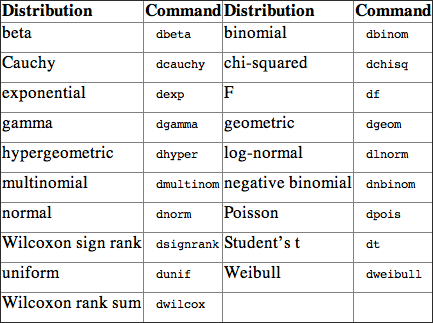
In addition to those listed in Table 1-1, R has commands to deal with the Studentized range: ptukey and qtukey.
Density Functions
The density/mass functions associated with these distributions are named dxxxx, where xxxx is the (abbreviated) name of the distribution. The distributions that R can deal with are listed previously in Table 1-1.
Command Name
dxxxxDensity/mass functions for various probability distributions (see Table 1-1). The individual commands are shown here:
dbeta
dbinom
dcauchy
dchisq
dexp
df
dgamma
dgeom
dhyper
dlnorm
dmultinom
dnbinom
dnorm
dpois
dsignrank
dt
dunif
dweibull
dwilcox
These commands provide access to the density computations for the various distributions. See the following examples for details of commonly used distributions.
Common Usage
dbeta(x, shape1, shape2, ncp, log = FALSE)
dbinom(x, size, prob, log = FALSE)
dcauchy(x, location = 0, scale = 1, log = FALSE)
dchisq(x, df, ncp = 0, log = FALSE)
dexp(x, rate = 1, log = FALSE)
df(x, df1, df2, ncp, log = FALSE)
dgamma(x, shape, rate = 1, scale = 1/rate, log = FALSE)
dgeom(x, prob, log = FALSE)
dhyper(x, m, n, k, log = FALSE)
dlnormal(x, meanlog = 0, sdlog = 1, log = FALSE)
dmultinom(x, size = NULL, prob, log = FALSE)
dnbinom(x, size, prob, mu, log = FALSE)
dnorm(x, mean = 0, sd = 1, log = FALSE)
dpois(x, lambda, log = FALSE)
dsignrank(x, n, log = FALSE)
dt(x, df, ncp, log = FALSE)
dunif(x, min = 0, max = 1, log = FALSE)
dweibull(x, shape, scale = 1, log = FALSE)
dwilcox(x, m, n, log = FALSE)
Related Commands
Command Parameters
| x | A vector of quantiles. |
| log = FALSE | If TRUE the probabilities are given as log(p). |
| Other parameters | Each distribution has its own set of parameters. |
Examples
The built-in R help entries for each distribution give details about the various commands. Following are some detailed examples on some of the more commonly used distributions.
Binomial Distribution
The binomial distribution requires size (the number of trials) and prob, the probability of success for each trial:
  ## Binomial density
> dbinom(0:5, size = 5, prob = 0.4)
[1] 0.07776 0.25920 0.34560 0.23040 0.07680 0.01024
Chi-Squared Distribution
The chi-squared distribution requires df (the degrees of freedom) and ncp, a non-centrality parameter (default ncp = 0):
  ## The chi-squared density for different degrees of freedom
> dchisq(1:5, df = 1)
[1] 0.24197072 0.10377687 0.05139344 0.02699548 0.01464498

> dchisq(1:5, df = 5)
[1] 0.08065691 0.13836917 0.15418033 0.14397591 0.12204152

  ## Use density to draw chi-squared distribution (see Figure 1-3)
> dcc = function(x) dchisq(x, df = 5) # Chi-Squared density
> curve(dcc, from = 0, to = 30) # Draw curve of chi-squared
> title(main = "Chi-squared distribution density function")
Figure 1-3: The chi-squared distribution plotted using the density function
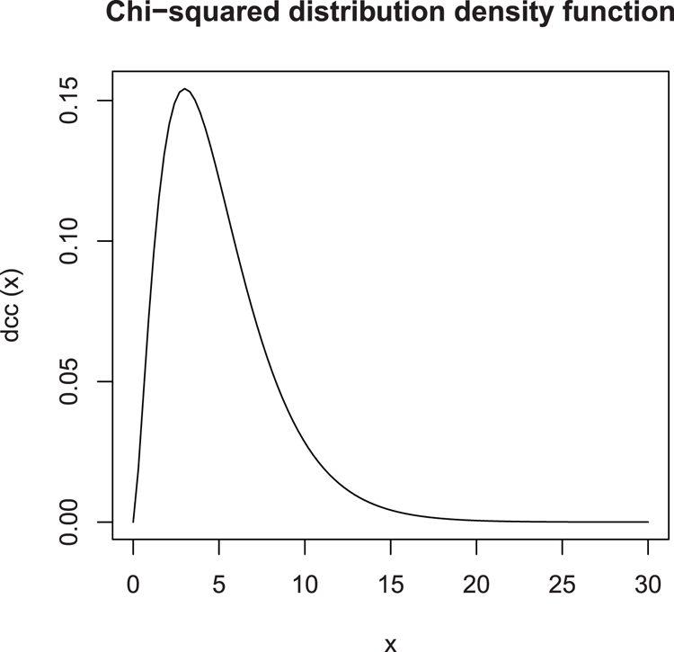
F Distribution
The F distribution requires degrees of freedom for numerator and denominator, df1 and df2, as well as ncp, a non-centrality parameter (if omitted, the central F is assumed):
  ## The F distribution density effects of df
> df(1:5, df1 = 1, df2 = 5)
[1] 0.21967980 0.09782160 0.05350733 0.03254516 0.02122066

> df(1:5, df1 = 2, df2 = 5)
[1] 0.30800082 0.12780453 0.06331704 0.03528526 0.02138334

> df(1:5, df1 = 1, df2 = 10)
[1] 0.23036199 0.10093894 0.05306663 0.03057288 0.01871043
Normal Distribution
The normal distribution requires the mean (default mean = 0) and sd (standard deviation, default sd = 1):
  ## Normal distribution density
> dnorm(1:5, mean = 0, sd = 1)
[1] 2.419707e-01 5.399097e-02 4.431848e-03 1.338302e-04 1.486720e-06

> dnorm(1:5, mean = 5, sd = 1.5)
[1] 0.007597324 0.035993978 0.109340050 0.212965337 0.265961520

  ## Use density function to draw distribution (see Figure 1-4)
> curve(dnorm, from = -4, to = 4) # Draw density function
> title(main = "Normal distribution density function") # Add title
Figure 1-4: The normal distribution plotted using the density function
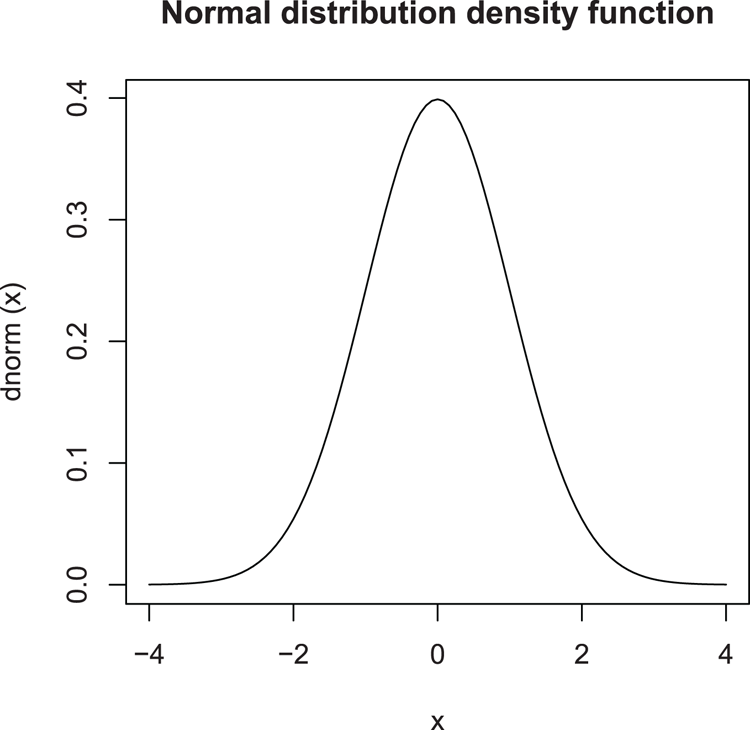
Poisson Distribution
The Poisson distribution requires lambda, a (non-negative) mean value.
  ## Poisson density for values 0-5
> dpois(0:5, lambda = 1, log = FALSE)
[1] 0.367879441 0.367879441 0.183939721 0.061313240 0.015328310 0.003065662

> dpois(0:5, lambda = 1, log = TRUE)
[1] -1.000000 -1.000000 -1.693147 -2.791759 -4.178054 -5.787492
Student’s t Distribution
The t distribution requires the degrees of freedom, df, and ncp, a non-centrality parameter (if omitted, the central t is assumed).
  ## Student’s t distribution, effects of degrees of freedom
> dt(1:5, df = 5)
[1] 0.219679797 0.065090310 0.017292579 0.005123727 0.001757438

> dt(1:5, df = 15)
[1] 0.234124773 0.059207732 0.009135184 0.001179000 0.000153436

> dt(1:5, df = Inf) # Set df to infinity
[1] 2.419707e-01 5.399097e-02 4.431848e-03 1.338302e-04 1.486720e-06
Probability Functions
The cumulative probability functions associated with these distributions are named pxxxx, where xxxx is the (abbreviated) name of the distribution. The distributions that R can deal with are listed in Table 1-1. The Studentized range is covered by the ptukey command.
Command Name
ecdfThis command creates a custom cumulative distribution. A vector of values is used as the basis for the custom distribution. The resulting object has special attributes, namely a class "ecdf". Dedicated summary and plot commands also exist for objects of the class "ecdf" (see the following examples).
Common Usage
ecdf(x)Related Commands
Command Parameters
| x | A vector of values. |
Examples
 ## Make a cumulative distribution
> myd = c(1,2,4,8,16,32,64,128,150,100,70,50,30,20,10,5,2,1) # Values
> myecdf = ecdf(myd) # Make a custom cumulative distribution

> Fn = myecdf # Make a primitive function
> Fn(myd) # Gives percentiles for myd
 [1] 0.1111111 0.2222222 0.2777778 0.3888889 0.5000000 0.6666667 0.7777778 0.9444444
 [9] 1.0000000 0.8888889 0.8333333 0.7222222 0.6111111 0.5555556 0.4444444 0.3333333
[17] 0.2222222 0.1111111

> class(myecdf) # Object holds several classes
[1] "ecdf"     "stepfun"  "function"

> ## Dedicated commands for class "ecdf"
> summary(myecdf) # Summary command
Empirical CDF:       16 unique values with summary
   Min. 1st Qu.  Median    Mean 3rd Qu.    Max.
   1.00    7.25   25.00   43.12   65.50  150.00

> plot(myecdf, verticals = TRUE, do.points = TRUE) # Plot (see Figure 1-5)
Figure 1-5: Plotting an “ecdf” object, a custom cumulative distribution
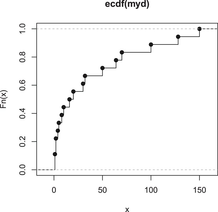
Command Name
ptukeyThe cumulative distribution of the Studentized range (often called Q). The Q statistic is often used in post-hoc analyses; for example, Tukey’s Honest Significant Difference.
Common Usage
ptukey(q, nmeans, df, lower.tail = TRUE, log.p = FALSE)Related Commands
Command Parameters
| q | A vector of quantiles. |
| nmeans | The number of groups. |
| df | The degrees of freedom; for post-hoc pairwise comparisons this is Inf. |
| lower.tail = TRUE | If TRUE (default), probabilities are given as P[X ≤ x]; if FALSE, P[X > x]. |
| log.p = FALSE | If TRUE, probabilities are given as log(p). |
Examples
  ## Some values for Q
> vec = seq(from = 3, to = 3.5, by = 0.1)
> vec # Show values
[1] 3.0 3.1 3.2 3.3 3.4 3.5

  ## Calculate probs for 3 grps, pairwise comparison
> ptukey(vec, nmeans = 3, df = Inf, lower.tail = FALSE)
[1] 0.08554257 0.07252045 0.06116000 0.05131091 0.04282463 0.03555704
Command Name
pxxxxCumulative probability functions for various probability distributions (see Table 1-1). The individual commands are shown here:
pbeta
pbinom
pcauchy
pchisq
pexp
pf
pgamma
pgeom
phyper
plnorm
pmultinom
pnbinom
pnorm
ppois
psignrank
pt
punif
pweibull
pwilcox
These commands provide access to the cumulative probability computations for the various distributions. See the following examples for details of commonly used distributions.
Common Usage
pbeta(q, shape1, shape2, ncp, lower.tail = TRUE, log.p = FALSE)
pbinom(q, size, prob, lower.tail = TRUE, log.p = FALSE)
pcauchy(q, location = 0, scale = 1, lower.tail = TRUE, log.p = FALSE)
pchisq(q, df, ncp = 0, lower.tail = TRUE, log.p = FALSE)
pexp(q, rate = 1, lower.tail = TRUE, log.p = FALSE)
pf(q, df1, df2, ncp, lower.tail = TRUE, log.p = FALSE)
pgamma(q, shape, rate = 1, scale = 1/rate, lower.tail = TRUE, log.p = FALSE)
pgeom(q, prob, lower.tail = TRUE, log.p = FALSE)
phyper(q, m, n, k, lower.tail = TRUE, log.p = FALSE)
plnormal(q, meanlog = 0, sdlog = 1, lower.tail = TRUE, log.p = FALSE)
pmultinom(q, size = NULL, prob, lower.tail = TRUE, log.p = FALSE)
pnbinom(q, size, prob, mu, lower.tail = TRUE, log.p = FALSE)
pnorm(q, mean = 0, sd = 1, lower.tail = TRUE, log.p = FALSE)
ppois(q, lambda, lower.tail = TRUE, log.p = FALSE)
psignrank(q, n, lower.tail = TRUE, log.p = FALSE)
pt(q, df, ncp, lower.tail = TRUE, log.p = FALSE)
punif(q, min = 0, max = 1, lower.tail = TRUE, log.p = FALSE)
pweibull(q, shape, scale = 1, lower.tail = TRUE, log.p = FALSE)
pwilcox(q, m, n, lower.tail = TRUE, log.p = FALSE)
Related Commands
Command Parameters
| q | A vector of quantiles. |
| lower.tail = TRUE | If TRUE, probabilities are P[X ≤ x]. If FALSE, P[X > x]. |
| log.p = FALSE | If TRUE, the probabilities are given as log(p). |
| Other parameters | Each distribution has its own set of parameters. |
Examples
The built-in R help entries for each distribution give details about the various commands. Following are some detailed examples on some of the more commonly used distributions.
Binomial Distribution
The binomial distribution requires size (the number of trials) and prob, the probability of success for each trial:
  ## Binomial cumulative distribution
> pbinom(0:5, size = 5, prob = 0.4)
[1] 0.07776 0.33696 0.68256 0.91296 0.98976 1.00000
Chi-Squared Distribution
The chi-squared distribution requires df (the degrees of freedom) and ncp, a non-centrality parameter (default ncp = 0):
  ## The chi-squared cumulative distribution for different degrees of freedom
> pchisq(1:10, df = 1)
 [1] 0.6826895 0.8427008 0.9167355 0.9544997 0.9746527 0.9856941 0.9918490
 [8] 0.9953223 0.9973002 0.9984346 0.9990889 0.9994680 0.9996885 0.9998172
[15] 0.9998925 0.9999367 0.9999626 0.9999779 0.9999869 0.9999923

> pchisq(1:20, df = 10)
 [1] 0.0001721156 0.0036598468 0.0185759362 0.0526530173 0.1088219811
 [6] 0.1847367555 0.2745550467 0.3711630648 0.4678964236 0.5595067149
[11] 0.6424819976 0.7149434997 0.7763281832 0.8270083921 0.8679381437
[16] 0.9003675995 0.9256360202 0.9450363585 0.9597373177 0.9707473119
F Distribution
The F distribution requires degrees of freedom for numerator and denominator, df1 and df2, as well as ncp, a non-centrality parameter (if omitted, the central F is assumed):
  ## The F cumulative probability distribution effects of df
> pf(1:10, df1 = 1, df2 = 5)
[1] 0.6367825 0.7835628 0.8561892 0.8980605 0.9244132 0.9420272 0.9543409
[8] 0.9632574 0.9699008 0.974969

> pf(1:10, df1 = 1, df2 = 10)
[1] 0.6591069 0.8123301 0.8860626 0.9266120 0.9506678 0.9657123 0.9755090
[8] 0.9820999 0.9866563 0.9898804
Normal Distribution
The normal distribution requires the mean (default mean = 0) and sd (standard deviation, default sd = 1):
  ## Normal cumulative distribution
> pnorm(0:5, mean = 0, sd = 1.5)
[1] 0.5000000 0.7475075 0.9087888 0.9772499 0.9961696 0.9995709

> pnorm(0:5, mean = 0, sd = 1.5, lower.tail = FALSE)
[1] 0.5000000000 0.2524925375 0.0912112197 0.0227501319 0.0038303806 0.0004290603
Poisson Distribution
The Poisson distribution requires lambda, a (non-negative) mean value:
  ## Poisson cumulative probability, effects of lambda
> ppois(0:5, lambda = 1)
[1] 0.3678794 0.7357589 0.9196986 0.9810118 0.9963402 0.9994058
> ppois(0:11, lambda = 5)
[1] 0.006737947 0.040427682 0.124652019 0.265025915 0.440493285 0.615960655
[7] 0.762183463 0.866628326 0.931906365 0.968171943 0.986304731 0.994546908
Student’s t Distribution
The t distribution requires the degrees of freedom, df, and ncp, a non-centrality parameter (if omitted, the central t is assumed):
  ## Student’s t cumulative probability
> pt(-1:5, df = 5, lower.tail = TRUE)
[1] 0.1816087 0.5000000 0.8183913 0.9490303 0.9849504 0.9948383 0.9979476

> pt(-1:5, df = 5, lower.tail = FALSE)
[1] 0.818391266 0.500000000 0.181608734 0.050969739 0.015049624 0.005161708
[7] 0.002052358
Quantile Functions
The quantile probability functions associated with these distributions are named qxxxx, where xxxx is the (abbreviated) name of the distribution. The distributions that R can deal with are listed in Table 1-1. The Studentized range is covered by the qtukey command.
Command Name
qtukeyCalculates quantiles for probabilities of the Studentized range (often called Q). The Q statistic is often used in post-hoc analyses; for example, Tukey’s Honest Significant Difference.
Common Usage
qtukey(p, nmeans, df, lower.tail = TRUE, log.p = FALSE)Related Commands
Command Parameters
| p | A vector of probabilities. |
| nmeans | The number of groups. |
| df | The degrees of freedom; for post-hoc pairwise comparisons this is Inf. |
| lower.tail = TRUE | If TRUE (default), probabilities are given as P[X ≤ x]; if FALSE, P[X > x]. |
| log.p = FALSE | If TRUE, probabilities are given as log(p). |
Examples
  ## Calculate critical values of Q for pairwise comparisons (groups 2-6)
> qtukey(0.95, nmeans = 2:6, df = Inf)
[1] 2.771808 3.314493 3.633160 3.857656 4.030092

> qtukey(0.99, nmeans = 2:6, df = Inf)
[1] 3.642773 4.120303 4.402801 4.602821 4.757047
Command Name
qxxxxQuantile functions for various probability distributions (see Table 1-1). The individual commands are shown here:
qbeta
qbinom
qcauchy
qchisq
qexp
qf
qgamma
qgeom
qhyper
qlnorm
qmultinom
qnbinom
qnorm
qpois
qsignrank
qt
qunif
qweibull
qwilcox
These commands provide access to the quantile computations for the various distributions. See the following examples for details of commonly used distributions.
Common Usage
qbeta(p, shape1, shape2, ncp, lower.tail = TRUE, log.p = FALSE)
qbinom(p, size, prob, lower.tail = TRUE, log.p = FALSE)
qcauchy(p, location = 0, scale = 1, lower.tail = TRUE, log.p = FALSE)
qchisq(p, df, ncp = 0, lower.tail = TRUE, log.p = FALSE)
qexp(p, rate = 1, lower.tail = TRUE, log.p = FALSE)
qf(p, df1, df2, ncp, lower.tail = TRUE, log.p = FALSE)
qgamma(p, shape, rate = 1, scale = 1/rate, lower.tail = TRUE, log.p = FALSE)
qgeom(p, prob, lower.tail = TRUE, log.p = FALSE)
qhyper(p, m, n, k, lower.tail = TRUE, log.p = FALSE)
qlnormal(p, meanlog = 0, sdlog = 1, lower.tail = TRUE, log.p = FALSE)
qmultinom(pq, size = NULL, prob, lower.tail = TRUE, log.p = FALSE)
qnbinom(p, size, prob, mu, lower.tail = TRUE, log.p = FALSE)
qnorm(p, mean = 0, sd = 1, lower.tail = TRUE, log.p = FALSE)
qpois(p, lambda, lower.tail = TRUE, log.p = FALSE)
qsignrank(p, n, lower.tail = TRUE, log.p = FALSE)
qt(p, df, ncp, lower.tail = TRUE, log.p = FALSE)
qunif(p, min = 0, max = 1, lower.tail = TRUE, log.p = FALSE)
qweibull(p, shape, scale = 1, lower.tail = TRUE, log.p = FALSE)
qwilcox(p, m, n, lower.tail = TRUE, log.p = FALSE)
Related Commands
Command Parameters
| p | A vector of probabilities. |
| lower.tail = TRUE | If TRUE, probabilities are P[X ≤ x]. If FALSE, P[X > x]. |
| log.p = FALSE | If TRUE, the probabilities are given as log(p). |
Examples
The built-in R help entries for each distribution give details about the various commands. Following are some detailed examples on some of the more commonly used distributions.
Binomial Distribution
The binomial distribution requires size (the number of trials) and prob, the probability of success for each trial:
  ## Binomial distribution, quantile function
> qbinom(c(0.3, 0.50, 0.9, 0.95, 0.99), size = 5, prob = 0.4)
[1] 1 2 3 4 5
Chi-Squared Distribution
The chi-squared distribution requires df (the degrees of freedom) and ncp, a non-centrality parameter (default ncp = 0):
  ## Critical values for chi-squared at 95% for df = 1-5
> qchisq(0.95, df = 1:5)
[1]  3.841459  5.991465  7.814728  9.487729 11.070498
F Distribution
The F distribution requires degrees of freedom for numerator and denominator, df1 and df2, as well as ncp, a non-centrality parameter (if omitted, the central F is assumed):
  ## Critical values for F at 95%
 > qf(0.95, df1 = 1, df2 = c(3, 5, 7, 9))
[1] 10.127964  6.607891  5.591448  5.117355
Normal Distribution
The normal distribution requires the mean (default mean = 0) and sd (standard deviation, default sd = 1):
  ## Critical values for various probabilities for the normal distribution
> qnorm(c(0.95, 0.98, 0.99, 0.999), mean = 0, sd = 1)
[1] 1.644854 2.053749 2.326348 3.090232
Poisson Distribution
The Poisson distribution requires lambda, a (non-negative) mean value:
  ## Poisson distribution critical values
> qpois(0.95, lambda = 1:5)
[1] 3 5 6 8 9

> qpois(0.99, lambda = 1:5)
[1]  4  6  8  9 11
Student’s t Distribution
The t distribution requires the degrees of freedom, df, and ncp, a non-centrality parameter (if omitted, the central t is assumed):
  ## Critical values for 95% (two-tailed) t distribution
 > qt(0.975, df = c(1, 3, 5, 10, Inf))
[1] 12.706205  3.182446  2.570582  2.228139  1.959964
Random Numbers
Random variates can be generated for many distribution types. The random variate functions associated with these distributions are named rxxxx, where xxxx is the (abbreviated) name of the distribution. The distributions that R can deal with are listed in Table 1-1. Control over random number generation is also provided by set.seed and RNGkind commands.
Command Name
RNGkindControls the way random numbers are generated. There are two kinds of generators; the first is the “regular” one and the second sets the generator for Normal generation. The RNGkind command can get or set the values that determine the algorithms used in generating random numbers.
Common Usage
RNGkind(kind = NULL, normal.kind = NULL)Related Commands
Command Parameters
| kind = NULL | A character string specifying the kind of generator to use. If NULL, the value is unchanged. If "default" is specified, the default is used: "Mersenne-Twister". If both kind and normal.kind are omitted or set to NULL, the current settings are displayed. |
| normal.kind = NULL | A character string specifying the kind of Normal generator to use. If NULL, the value is unchanged. If "default" is specified, the default is used: "Inversion". If both kind and normal.kind are omitted or set to NULL, the current settings are displayed. |
Examples
  ## Random Number Generators
> RNGkind() # See current generators
[1] "Mersenne-Twister" "Inversion"

  ## Set to new generators
> RNGkind(kind = "Super-Duper", normal.kind = "Box-Muller")
> RNGkind() # Check to see current generators
[1] "Super-Duper" "Box-Muller"

  ## Set new generator but leave Normal generator "as is"
> RNGkind(kind = "Wichmann-Hill", normal.kind = NULL)
> RNGkind() # Check generators
[1] "Wichmann-Hill" "Box-Muller"

  ## Reset R default generators
> RNGkind(kind = "default", normal.kind = "default")
> RNGkind() # Check generators
[1] "Mersenne-Twister" "Inversion"
Command Name
rxxxxRandom number generation functions for various probability distributions (see Table 1-1). The individual commands are shown here:
rbeta
rbinom
rcauchy
rchisq
rexp
rf
rgamma
rgeom
rhyper
rlnorm
rmultinom
rnbinom
rnorm
rpois
rsignrank
rt
runif
rweibull
rwilcox
These commands provide access to random variate generation for the various distributions. See the following examples for details of commonly used distributions. The runif command produces random numbers for the uniform distribution, that is, regular numbers.
Common Usage
rbeta(n, shape1, shape2, ncp)
rbinom(n, size, prob)
rcauchy(n, location = 0, scale = 1)
chisq(n, df, ncp = 0)
rexp(n, rate = 1)
rf(n, df1, df2, ncp)
rgamma(n, shape, rate = 1, scale = 1/rate
rgeom(n, prob)
rhyper(nn, m, n, k)
rlnormal(n, meanlog = 0, sdlog = 1)
rmultinom(n, size = NULL, prob)
rnbinom(n, size, prob, mu)
rnorm(n, mean = 0, sd = 1)
rpois(n, lambda)
rsignrank(nn, n)
rt(n, df, ncp)
runif(n, min = 0, max = 1)
rweibull(n, shape, scale = 1)
rwilcox(x, m, n)
Related Commands
Command Parameters
| n | The number of random numbers to generate. For rhyper and rsignrank the parameter is nn, because n refers to something else (# black balls or # in sample, respectively). |
| Other parameters | Each distribution has its own set of parameters. |
Examples
The built-in R help entries for each distribution give details about the various commands. Following are some detailed examples on some of the more commonly used distributions.
Binomial Distribution
The binomial distribution requires size (the number of trials) and prob, the probability of success for each trial:
  ## Random numbers from the binomial distribution
> set.seed(5) # Set random number seed
> rbinom(10, size = 5, prob = 0.4)
 [1] 1 3 4 1 1 3 2 3 4 1
Chi-Squared Distribution
The chi-squared distribution requires df (the degrees of freedom) and ncp, a non-centrality parameter (default ncp = 0):
  ## Random variates from the chi-squared distribution
set.seed(5) # Set random number seed
> rchisq(5, df = 1)
[1] 0.11237767 3.25084859 0.03070214 0.78143200 4.54600483

> set.seed(5) # Set random number seed again
> rchisq(5, df = 5)
[1]  1.975221  2.550650  4.200854 10.305201  2.476468
Normal Distribution
The normal distribution requires the mean (default mean = 0) and sd (standard deviation, default sd = 1):
  ## Random numbers from the normal distribution
> set.seed(5) # Set the random number seed
> rnorm(5, mean = 0, sd = 1)
[1] -0.84085548  1.38435934 -1.25549186  0.07014277  1.71144087

> set.seed(5) # Set the random number seed
> rnorm(5, mean = 5, sd = 1)
[1] 4.159145 6.384359 3.744508 5.070143 6.711441
Poisson Distribution
The Poisson distribution requires lambda, a (non-negative) mean value:
  ## Random values from the Poisson distribution
> set.seed(5) # Set the random number seed
> rpois(5, lambda = 1)
[1] 0 1 2 0 0

> set.seed(5) # Set the random number seed
> rpois(5, lambda = 5)
[1] 3 6 8 4 2
Uniform Distribution
This is what you would think of as “regular” numbers. The command requires min and max parameters, which set the minimum and maximum values for the random values:
  ## Random values from the uniform distribution
> set.seed(5) # Set the random number seed
> runif(5, min = 0, max = 100)
[1] 20.02145 68.52186 91.68758 28.43995 10.46501

> set.seed(5) # Set the random number seed
> runif(5, min = 1, max = 9)
[1] 2.601716 6.481749 8.335006 3.275196 1.837201
Command Name
set.seedSets the random number seed. Think of this as setting the starting point for the generation of random numbers. If you set this to a particular value, you will get the same results each time you run a command that generates random values; this is useful for testing and teaching purposes.
Common Usage
set.seed(seed, kind = NULL, normal.kind = NULL)Related Commands
Command Parameters
| seed | A single value (an integer), which sets the starting point for the random seed generator. |
| kind = NULL | Sets the random number generator to one of the options. If NULL, the currently set option is used (see: RNGkind). If "default" is used, the default setting is used, which is "Mersenne-Twister". |
| normal.kind = NULL | Sets the method of Normal generation. If NULL, the current setting is used (see: RNGkind). If "default", the default setting is used, which is "Inversion". |
Examples
  ## Random numbers
> set.seed(1) # Start with a seed value
> runif(5) # Five values from uniform distribution
[1] 0.2655087 0.3721239 0.5728534 0.9082078 0.2016819

> set.seed(10) # Use a new seed
> runif(5) # Five new random values
[1] 0.50747820 0.30676851 0.42690767 0.69310208 0.08513597

> set.seed(1) # Set seed to earlier value
> runif(5) # Five more values, match the earlier result
[1] 0.2655087 0.3721239 0.5728534 0.9082078 0.2016819

> set.seed(1, kind = "Super-Duper") # Use the "Super-Duper" generator
> runif(5) # Five more values
[1] 0.3714075 0.4789723 0.9636913 0.6902364 0.6959049

> RNGkind() # Check to see what generators are set
[1] "Super-Duper" "Inversion"

> set.seed(1) # Start seed again, sets to current generator
> runif(5) # Five more values
[1] 0.3714075 0.4789723 0.9636913 0.6902364 0.6959049

> set.seed(1, kind = "default") # Set seed, uses default "Mersenne-Twister"
> runif(5) # Five more values, match earlier result
[1] 0.2655087 0.3721239 0.5728534 0.9082078 0.2016819