Theme 4: Utilities
This theme covers the commands that are generally useful when accessing the programming aspect of the R language. This theme also covers some commands that do not easily fit into the other three themes of “Data,” “Math and Statistics,” and “Graphics.” Some of these topics include accessing the help system and getting/using additional packages of R commands.
Because R is a programming language, you have great flexibility in how you use it. You can customize R in two main ways:
- Custom functions
- Scripts (used as source code)
These two methods differ from one another in the following manner: You can think of functions as short scripts you can type from the keyboard and scripts as longer items that you would use a text editor to create. Once you start to create and use your own custom functions and scripts, you will need to use certain commands that help you undertake the tasks you set R to do and to manage the output (so you can see the results).
Topics in this Theme
Commands In This Theme:
Install
The R website at www.r-project.org is a vast repository of all things R-related. This includes the program itself (for all operating systems) as well as additional packages of R commands. The basic installation of R is very powerful, but it can be extended even further by the addition of extra packages of commands (at the time of this writing there were nearly 4000 packages). These packages have been written to carry out a bewildering variety of things. You can browse the R website to see what is available; the Task Views section of the website is very useful because it covers most of the available packages in a topic-based manner. An Internet search will also prove useful if you have a specific topic in mind.
What’s In This Topic:
- Installing new additional packages
- Updating packages
Installing R
The source for all R program installers is the website www.r-project.org, where you can find the appropriate version for your computer. You will need to select a mirror site; choose one local to you to minimize download time. Generally, the link you follow takes you to a page where you can select the version you require. The main program files are called the R binaries, whereas additional packages are simply referred to as packages.
The installation process will vary according to your operating system; for Windows or Mac it is usually just a matter of running the installation file that you download. For Linux the process may be slightly more complicated, but the website gives instructions.
Installing Packages
Many packages of additional R commands are available for you to use to extend the capabilities of R. The first step is to identify the package you need. The R website at www.r-project.org is a good place to browse the options and the Task Views section gives you a topic-based way of finding what you may need. Once you know the name of the package you require, you can use the appropriate command in R to get and install it.
It is possible to use menu commands if you have Windows or Mac versions of R (using the Packages menu), but it is easier to type the command!
Command Name
install.packagesThis command installs a package from the R website onto your computer. You need to be connected to the Internet to download a file, or you can optionally point to a file on your computer if it is already downloaded.
Common Usage
install.packages(pkgs, repos = getOption(“repos”), dependencies = NA)Related Commands
Command Parameters
| pkgs | The packages to install. You must give a character vector of the names. If repos = NULL, you can “point” to a file on your computer by specifying the path (in quotes). |
| repos | A character vector pointing to the repository for the installation files: this can be a URL. The default asks you for a location to select (your mirror site). If you set repos = NULL, you can install a file from an archive on your computer. |
| dependencies = NA | Some packages require that others be installed before they will work correctly. The default, NA, installs these other packages. You can also specify TRUE or FALSE. |
Examples
  ## Install a single package from the Internet
> install.packages(“gdata”)

  ## Multiple packages can be installed
> install.packages(c(“ade4”, “vegan”))
Command Name
new.packages
old.packages
update.packages
These commands help you to manage the installation of packages:
- new.packages checks for packages that are not already installed and offers to install them.
- old.packages checks for packages that are already installed but which have newer versions.
- update.packages checks for package updates and offers to install them.
Common Usage
new.packages(repos = getOption(“repos”), ask = FALSE)

old.packages(repos = getOption(“repos”))

update.packages(repos = getOption(“repos”), ask = TRUE)
Related Commands
Command Parameters
| repos | A character vector pointing to the repository for the installation files; this can be a URL. The default asks you for a location to select (your local mirror site). If you set repos = NULL, you can install a file from an archive on your computer. |
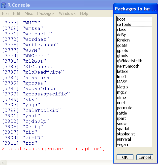
| ask | If ask = TRUE, the user is asked to confirm the installation of each available package. You can also specify “graphics”, which brings up an interactive list that enables you to select the packages you want. |
Examples
  ## Interactive update using Windows OS (Figure 4-1)
> update.packages(ask = "graphics")
Figure 4-1: Interactive selection of packages to update
Using R
Some commands help your day-to-day operation of R. This topic is concerned with those useful commands and covers several broad themes: the help system and previously typed commands, saving your work (and getting it back), and the management of additional packages.
What’s In This Topic:
- The help system
- Previous command history
- Saving work
- Quitting R
- Opening Packages
- Closing Packages
Using the Program
Command Name
apropos
find
These commands find objects by partial matching of their names. The main use for apropos is to find commands for which you cannot recall the exact name. The find command shows where the object is located in the search environment.
Common Usage
apropos(what, where = FALSE, ignore.case = TRUE, mode = "any")

find(what, mode = "any", numeric = FALSE, simple.words = TRUE)
Related Commands
Command Parameters
| what | A character string giving the name to match. For apropos you can also use a regular expression. |
| where = FALSEnumeric = FALSE | If TRUE, the position on the search path is also indicated. |
| ignore.case = TRUE | By default, the matching is not case sensitive. |
| mode = “any” | The default is to match objects of any type. If you want to search only for a certain type of object, you must give the mode as a character string. |
| simple.words = TRUE | Matches only complete words. For partial matching, use simple.words = FALSE. |
Examples
  ## Show the search path
> search()
 [1] ".GlobalEnv"        "tools:RGUI"        "package:stats"
 [4] "package:graphics"  "package:grDevices" "package:utils"
 [7] "package:datasets"  "package:methods"   "Autoloads"
[10] "package:base"

  ## Partial match for “mean”
> apropos("mean")
 [1] "colMeans"       "kmeans"         "mean"            "mean.Date"
 [5] "mean.POSIXct"   "mean.POSIXlt"   "mean.data.frame" "mean.default"
 [9] "mean.difftime"  "mean.fw"        "rowMeans"        "weighted.mean"

  ## The find command returns the search path
> find("mean", simple.words = FALSE, numeric = TRUE)
package:stats  package:base
            3            10

  ## Use a regular expression
> apropos("^fw")
 [1] "fw"      "fw.cm"   "fw.cov"  "fw.list" "fw.lm"   "fw.mat"  "fw1"
 [8] "fw2"     "fw3"     "fwe"     "fwi"     "fws"

  ## For find, regular expression works only if simple.words = FALSE
> find("^fw", simple.words = FALSE)
[1] ".GlobalEnv"
Command Name
help
?
help.start
These commands provide access to the help system. The ? is a helper function for the help command and provides a quick way to access help on a particular topic. The help.start command opens a web browser and loads the help index so that you can navigate through the help system. You do not need to be connected to the Internet.
Common Usage
help(topic, package = NULL,
     try.all.packages = getOption(“help.try.all.packages”),
     help_type = getOption(“help_type”))

?topic

help.start()
Related Commands
Command Parameters
| topic | The topic for which help is required. This should be a character string for the help command, but you can omit the quotation marks by using ?topic. |
| package = NULL | The name of the package as a character string. This allows access to the help entry even if the package is not on the search path (e.g., has not been opened using the library command). |
| try.all.packages | The general default is that only packages on the search path are searched for a matching help topic. If TRUE, all packages are searched. |
| help_type | The default help display method will vary according to your OS. You can attempt to override the default by supplying a character string. The options include “text”, “html”, and “pdf”. |
Examples
  ## Open the help entry on the mean command using the default
> help("mean")

  ## Also brings up help entry for mean command
> ?mean

  ## This command is not in the current search path
> ?fitdistr
No documentation for 'fitdistr' in specified packages and libraries:
you could try '??fitdistr'

  ## This searches all packages and
 ## gives an indication of where the command can be found
> ??fitdistr

  ## Look for the command in all packages
> help("fitdistr", try.all.packages = TRUE)

  ## Once you know the package you can get the help entry even if
  ## the package is not currently loaded on the search path
> help("fitdistr", package = "MASS")
Command Name
history
savehistory
loadhistory
timestamp
These commands provide a way to access and manage the history of previously typed commands. You can also use the up and down arrows to navigate through the list of previously typed commands.
- history shows the last few commands typed.
- savehistory saves the current history of commands to a disk file as plain text.
- loadhistory loads a set of commands into the history.
- timestamp saves a timestamp to the current history.
Common Usage
loadhistory(file = ".Rhistory")
savehistory(file = ".Rhistory")

history(max.show = 25, reverse = FALSE, pattern, ignore.case = FALSE)

timestamp()
Related Commands
Command Parameters
| file | A filename, which must be in quotes. The current working directory is used unless given explicitly. On an OS other than Linux you can use file.choose() instead of a filename to read. The file saved/read is plain text, so you can edit or create a history file using a plain text editor. |
| max.show = 25 | By default, only the first 25 entries in the history file are shown. |
| reverse = FALSE | If you want the latest entry at the top of the list, use reverse = TRUE. |
| pattern | A pattern in the form of a regular expression to match in the history list. |
| ignore.case = FALSE | By default, any pattern is case sensitive. |
Examples
  ## What is the current working directory?
> getwd()
[1] "/Users/markgardener"

  ## Save the current history to a file in the working directory
> savehistory(file = "My_Working_History.RHistory")

  ## Show last 125 entries in history file
> history(max.show = 125)

  ## Use pattern matching
> history(pattern = "barplot")
> history(pattern = "^plot")
> history(pattern = "barplot", reverse = TRUE)
Command Name
quit
q
These commands exit R. The q command is an alias for quit. The command usually offers to save the current workspace. However, this setting may have been altered so you can choose to override the current default. Optionally, you can create a custom function called .Last, which is executed on quitting.
Common Usage
quit(save = "default", runLast = TRUE)
   q(save = "default", runLast = TRUE)

.Last <- function(x) { ...... }
Related Commands
Command Parameters
| save = “default” | A character string giving one of the options “no”, “yes”, “ask”, or “default”. This determines if the workspace is saved to disk. The default is usually “ask”. |
| runLast = TRUE | You can create a custom function called .Last, which is executed on quitting by default. To not run the function, use runLast = FALSE. |
| { ......} | Any valid R command or set of commands. The custom function .Last is executed when you quit R. |
Examples
  ## Quits R in the normal way and
  ## asks for save of workspace if that is the default
> q()

  ## Make sure you save current workspace
> q(save = "yes")

  ## Set up a function
  ## Simply displays a message to screen
> .Last = function(x) {cat("Goodbye..")}

  ## Quit R but don’t run .Last function
> q(runLast = FALSE)
Command Name
save.imageThis command saves the current workspace to disk.
Common Usage
save.image()Related Commands
Additional Packages
Many packages of additional R commands are available for you to use to extend the capabilities of R.
Command Name
detachThis command detaches a package from the search path. This makes the commands within that package unavailable.
Common Usage
detach(package:pkgname)Related Commands
Command Parameters
| package:pkgname | The name of the package. You must give this as a character string; see the following examples. |
Examples
  ## View the search path to see the MASS package is loaded
> search()
 [1] ".GlobalEnv"        "package:MASS"      "tools:RGUI"
 [4] "package:stats"     "package:graphics"  "package:grDevices"
 [7] "package:utils"     "package:datasets"  "package:methods"
[10] "Autoloads"         "package:base"

  ## Detach the MASS package
> detach("package:MASS")
Command Name
installed.packagesThis command shows a list of all the packages currently installed. The result can be very extensive if you have a lot of packages installed on your system. You can also use library(pkg), if the package is not installed, the command will fail.
Common Usage
installed.packages()Related Commands
Command Parameters
| () | If no parameters are given, the command searches all the library locations to list packages. |
Examples
  ## Get the list of installed packages and save result (it is a matrix)
> ip = installed.packages()

  ## See the headings of the result
> colnames(ip)
 [1] "Package"   "LibPath"   "Version"   "Priority" "Depends"  "Imports"
 [7] "LinkingTo" "Suggests"  "Enhances"  "OS_type"  "License"  "Built"

  ## View the first 5 rows for the “Package” column (the name)
> ip[1:5, "Package"]
      abind    accuracy        ade4   ade4TkGUI    adegenet
    "abind"  "accuracy"      "ade4" "ade4TkGUI"  "adegenet"

  ## The fifth column shows the dependencies, that is
  ## the other packages that must be loaded for them to work
> ip[1:5, c(1,5)]
          Package     Depends
abind     "abind"     "R (>= 1.5.0)"
accuracy  "accuracy"  NA
ade4      "ade4"      NA
ade4TkGUI "ade4TkGUI" "ade4 (>= 1.4-3), tcltk"
adegenet  "adegenet"  "methods, MASS"
Command Name
library
require
These commands load additional packages of commands. The require command is intended to be called by other commands because it returns a warning, rather than an error, if the package does not exist.
Common Usage
library(package)
return(package)
Related Commands
Command Parameters
| package | The name of the package to load. This can be a character string or the name of the package without quotation marks. |
Examples
  ## Examine the search path (shows the packages loaded)
> search()
 [1] ".GlobalEnv"        "tools:RGUI"        "package:stats"
 [4] "package:graphics"  "package:grDevices" "package:utils"
 [7] "package:datasets"  "package:methods"   "Autoloads"
[10] "package:base"

  ## Load the “MASS” package
> library(MASS)

Attaching package: 'MASS'
Warning message:
package 'MASS' was built under R version 2.12.2

  ## Turn off warning messages
> options("warn" = -1)

  ## Attempt to load a non-existent package
> library(zzz)
Error in library(zzz) : there is no package called 'zzz'

  ## Attempt to load a non-existent package
> require(zzz)
Loading required package: zzz

  ## Examine search path, zzz package not loaded!
> search()
 [1] ".GlobalEnv"        "package:MASS"      "tools:RGUI"
 [4] "package:stats"     "package:graphics"  "package:grDevices"
 [7] "package:utils"     "package:datasets"  "package:methods"
[10] "Autoloads"         "package:base"

  ## Reset warnings
> options("warn" = 0)
Command Name
search
searchpaths
These commands show the search path. Essentially, this lists the packages that are currently loaded and any data frames (or other objects) that have been added to the path using the attach command. The search command shows a simple list of names and the searchpaths command shows the library locations in addition to the names.
Common Usage
search()

searchpaths()
Related Commands
Command Parameters
| () | No parameters are required. |
Examples
  ## Examine the current search path
> search()
[1] ".GlobalEnv"        "tools:RGUI"         "package:stats"
 [4] "package:graphics"  "package:grDevices" "package:utils"
 [7] "package:datasets"  "package:methods"   "Autoloads"
[10] "package:base"

  ## Load the MASS library
> library(MASS)

Attaching package: 'MASS'
Warning message:
package 'MASS' was built under R version 2.12.2

  ## Make a simple data frame
> dat = data.frame(col1 = 1:3, col2 = 4:6)

  ## Attach the dat data object
> attach(dat)

  ## Look at the search path again
> search()
[1] ".GlobalEnv" "dat" "package:MASS" "tools:RGUI"
[5] "package:stats" "package:graphics" "package:grDevices" "package:utils"
[9] "package:datasets" "package:methods" "Autoloads" "package:base"
## An alternative view of the search path
> searchpaths()
[1] ".GlobalEnv"
[2] "pw"
[3] "/Library/Frameworks/R.framework/Versions/2.12/Resources/library/MASS"
[4] "tools:RGUI"
[5] "/Library/Frameworks/R.framework/Versions/2.12/Resources/library/stats"
[6] "/Library/Frameworks/R.framework/Versions/2.12/Resources/library/graphics"
[7] "/Library/Frameworks/R.framework/Versions/2.12/Resources/library/grDevices"
[8] "/Library/Frameworks/R.framework/Versions/2.12/Resources/library/utils"
[9] "/Library/Frameworks/R.framework/Versions/2.12/Resources/library/datasets"
[10] "/Library/Frameworks/R.framework/Versions/2.12/Resources/library/methods"
[11] "Autoloads"
[12] "/Library/Frameworks/R.framework/Resources/library/base"
  ## Tidy up – remove items from search path
> detach(dat)
> detach("package:MASS")
Programming
Programming R yourself can be especially useful because in doing so you can prepare scripts that undertake complex or repetitive tasks, which can be brought into operation at any time. Indeed, R is built along these (modular) lines and you can think of R as a bundle of scripts; by making your own you are simply increasing the usefulness of R and bending it to meet your own specific requirements.
This topic contains commands that are especially connected with the production of scripts—you are more likely to encounter the commands in this context than in any other.
What’s In This Topic:
- Producing output
- User intervention
- Text functions
Managing Functions
R provides various commands that help you to manage the functions that you create, enabling you to list the custom functions or to see the required arguments, for example.
Command Name
argsThis command displays the arguments required for a named function. Any default values are also displayed.
Common Usage
args(name)Related Commands
Command Parameters
| name | The name of the function or command. Usually you can simply give the name, but a character string is also accepted. |
Examples
  ## Make a 1-line function (there are 3 arguments, one has a default value)
> manning = function(radius, grad, coef = 0.1125) (radius^(2/3)*grad^0.5/coef)

  ## Make a multi-line function (returns the running median of a vector, x)
> cummedian = function(x) {
   tmp = seq_along(x)
   for(i in 1:length(tmp)) tmp[i] = median(x[1:i])
   print(tmp)
 }

  ## Look at arguments (user input)
> args(manning)
function (radius, grad, coef = 0.1125)
NULL

> args(cummedian)
function (x)
NULL

## Show arguments for a built-in function/command, bxp
> args("bxp")
function (z, notch = FALSE, width = NULL, varwidth = FALSE, outline = TRUE,
    notch.frac = 0.5, log = "", border = par("fg"), pars = NULL,
    frame.plot = axes, horizontal = FALSE, add = FALSE, at = NULL,
    show.names = NULL, ...)
NULL
Command Name
bodyThis command shows the body of a function; that is, “how it works.” You can also alter the function, but this is sensible only for fairly short code snippets.
Common Usage
body(fun)
body(fun) <- value
Related Commands
Command Parameters
| fun | The name of the function or command. Usually you can simply give the name, but a character string is also accepted. |
| value | The new body for the function. You must be careful that this is not evaluated, so you generally have to use a quote or expression. |
Examples
  ## Make a multi-line function
  ## (returns the running median of a vector, x)
> cummedian = function(x) {
   tmp = seq_along(x)
   for(i in 1:length(tmp)) tmp[i] = median(x[1:i])
   print(tmp)
 }

## View the main body of the function
> body(cummedian)
{
    tmp = seq_along(x)
    for (i in 1:length(tmp)) tmp[i] = median(x[1:i])
    print(tmp)
}

## A simple trivial function
> f = function(x) x^5

  ## View main body
> body(f)
x^5

> f(2)
[1] 32

  ## Change body, note that quote is used
  ## to prevent x being evaluated as an object
> body(f) <- quote(5^x)

  ## Check the new body
> body(f)
5^x

> f(2)
[1] 25
Command Name
formalsThis command allows access to the arguments of a function and permits you to alter the default values.
Common Usage
formals(fun)
formals(fun) <- value
Related Commands
Command Parameters
| fun | The name of a function. If you are simply looking at the arguments, you can use a character string. |
| value | A list giving the arguments and their default values. If no default is to be used, specify NULL. Alternatively, you can use alist (see the following examples). |
Examples
  ## Make a 1-line function
> manning = function(radius, grad, coef = 0.1125) (radius^(2/3)*grad^0.5/coef)

  ## Examine the formal arguments
> formals(manning)
$radius

$grad

$coef
[1] 0.1125

  ## Alter defaults
> formals(manning) <- list(radius = NULL, grad = NULL, coef = 0.21)

  ## View function
> manning
function(radius, gradient, coef = 0.1125) (radius^(2/3)*gradient^0.5/coef)

  ## Run function but miss out an argument..
  ## ..no result
> manning(2)
numeric(0)

  ## Alter formals but use alist instead (NULL now not needed)
  ## Note all arguments must be listed
> formals(manning) <- alist(radius = , grad = , coef = 0.21)

  ## Run function, missing value now produces an informative error
> manning(2)
Error in grad^0.5 : 'grad' is missing

  ## Use formals to create a function from a template
> func = function(x) a + b

  ## This function will not work as it is because a and b do not exist
  ## Create default values for function
  ## (a: unspecified, b: default value = 3)
> formals(func) <- alist(a = , b = 3)

  ## View the function
> func
function (a, b = 3)
a + b

  ## Run function
> func(a = 2)
[1] 5
Command Name
functionThis command creates custom functions. A function is a collection of R commands that are bundled together in a named object (a function or custom command). You can create simple functions directly from the keyboard. When your functions become more complicated, you are more likely to use a text editor to write the source code.
Common Usage
function(arglist) exprRelated Commands
Command Parameters
| arglist | A list of named arguments. Default values for arguments are given as arg = value. |
| expr | The expression(s) to be evaluated as part of the function. Essentially this is a series of R commands, using the arguments given in the arglist. If your function is more than one line, it is common to enclose the expr in braces (curly brackets). Braces are also used to separate sections of code (in conditional statements, for example). Once functions become larger than just a few lines, it is generally easier to use a text/script editor and use source to read them into R. |
Examples
  ## A simple function
> func = function(x) x^3

  ## View the function
> func
function(x) x^3

  ## Run the function
> func(3)
[1] 27

  ## Make a 1-line function; one argument has a default value
> manning = function(radius, grad, coef = 0.1125) (radius^(2/3)*grad^0.5/coef)
  ## Run the function (calculate speed of water)
> manning(radius = 1, grad = 0.1)
[1] 2.810913

  ## Make a multi-line function; use {} to allow
  ## multiple lines of code to be typed into the console
> cummedian = function(x) {
   tmp = seq_along(x)
   for(i in 1:length(tmp)) tmp[i] = median(x[1:i])
   print(tmp)
 }

  ## Run the function (cumulative median)
> cummedian(1:10)
 [1] 1.0 1.5 2.0 2.5 3.0 3.5 4.0 4.5 5.0 5.5
Command Name
lsf.strThis command shows the structure of functions at a specified position in the search path.
Common Usage
lsf.str(pos = -1)Related Commands
Command Parameters
| pos = -1 | The position of the environment to use for the listing as given by the search command. The default pos = -1 and pos = 1 are equivalent and relate to the global environment (the workspace). Other positions relate to various command packages. |
Examples
  ## Make some simple functions
> func = function(x) x^3

> manning = function(radius, grad, coef = 0.1125) (radius^(2/3)*grad^0.5/coef)

> cummedian = function(x) {
    tmp = seq_along(x)
    for(i in 1:length(tmp)) tmp[i] = median(x[1:i])
    print(tmp)
  }

  ## View the search path
> search()
 [1] ".GlobalEnv"        "tools:rstudio"     "package:stats"
 [4] "package:graphics"  "package:grDevices" "package:utils"
 [7] "package:datasets"  "package:methods"   "Autoloads"
[10] "package:base"

  ## View functions in the Global Environment (“user functions”)
> lsf.str(pos = -1)
cummedian : function (x)
func : function (x)
manning : function (radius, gradient, coef = 0.1125)

  ## Functions in position 2 (Mac OS X GUI)
> lsf.str(pos = 2)
browse.pkgs : function (repos = getOption("repos"),
    contriburl = contrib.url(repos, type), type = getOption("pkgType"))
data.manager : function ()
main.help.url : function ()
package.manager : function ()
print.hsearch : function (x, ...)
q : function (save = "default", status = 0, runLast = TRUE)
quartz.save : function (file, type = "png", device = dev.cur(),
    dpi = 100, ...)
quit : function (save = "default", status = 0, runLast = TRUE)
Rapp.updates : function ()
Saving and Running Scripts
You can create scripts by one of several methods. The simplest is to type the commands that make up the script directly into the console window. This is most useful for simple functions that are only a few lines at most. For longer and more complicated functions/scripts, it is better to use a dedicated text editor. Windows and Mac users have script editors built into the R GUI. Your scripts will be in two forms, plain text or R-encoded binary files:
- Scripts that are plain text can be read into R using the source command.
- Custom functions that you save as binary files using the save command can be read into R using the load command.
Command Name
dumpThis command attempts to write a text representation of R objects to disk. The resulting file can often be opened using the source command. This is not always entirely successful, depending on the nature of the object(s) being handled.
Common Usage
dump(list, file = “dumpdata.R”, append = FALSE, control = “all”)Related Commands
Command Parameters
| list | A character vector containing the names of the R objects to be written. |
| file = “dumpdata.R” | The filename in quotes; if blank, the output goes to current device (usually the screen). Filename defaults to the current working directory unless specified explicitly. Can also link to URL. For Windows and Mac OS the filename can be replaced by file.choose(), which brings up a file browser. |
| append = FALSE | If the output is a file, append = TRUE adds the result to the file; otherwise, the file is overwritten. |
| control = “all” | Controls the deparsing process. Use control = “all” for the most complete deparsing. Other options are “keepNA”, “keepInteger”, “showAttributes”, and “useSource”. Use control = NULL for the simplest representation. |
Examples
  ## Make a multi-line function
> cummedian = function(x) {
   tmp = seq_along(x)
   for(i in 1:length(tmp)) tmp[i] = median(x[1:i])
   print(tmp)
 }

  ## Write the function to disk as text
  ## .R file extension is associated with R scripts
> dump(ls(pattern = "cummedian"), file = "My_Function.R")

  ## Remove function from R
> rm(cummedian)

  ## Restore function from disk
> source(file = "My_Function.R")
Command Name
loadThis command reloads data that was saved from R in binary format (usually via the save command). The save command creates a binary file containing named R objects, which may be data, results, or custom functions. The load command reinstates the named objects, overwriting any identically named objects with no warning.
Common Usage
load(file)Related Commands
Command Parameters
| file | The filename in quotes. Defaults to the current working directory unless specified explicitly. Can also link to URL. For Windows and Mac OS the filename can be replaced by file.choose(), which brings up a file browser. |
Examples
  ## Make a function
> cummedian
function(x) {
  tmp = seq_along(x)
  for(i in 1:length(tmp)) tmp[i] = median(x[1:i])
  print(tmp)
}

  ## Save function to disk as binary file
  ## .RData file is associated with R binary files
> save(cummedian, file = "My_Function_Save.RData")

  ## Remove original from console
> rm(cummedian)

  ## Load function from binary disk file
> load("My_Function_Save.RData")
Command Name
saveThis command saves R objects to disk as binary encoded files (that is, not plain text). The objects saved with the save command can be loaded using the load command.
Common Usage
save(..., list = character(0L), file = stop(“‘file’ must be specified”),
     ascii = FALSE)
Related Commands
Command Parameters
| ... | Names of R objects (separated by commas) to be saved. |
| list = | A list can be given instead of explicit names; this allows the ls command to be used, for example. |
| file = | The filename in quotes; defaults to the current working directory unless specified explicitly. Can also link to URL. For Windows and Mac OS the filename can be replaced by file.choose(), which brings up a file browser. |
| ascii = FALSE | If set to TRUE, an ASCII representation is written to disk. This is not the same as “saving a text file,” but rather uses ASCII encoding instead of a binary code. The resulting file can still be opened using the load command. |
Examples
  ## Make a function
> cummedian
function(x) {
  tmp = seq_along(x)
  for(i in 1:length(tmp)) tmp[i] = median(x[1:i])
  print(tmp)
}

  ## Save function to disk as binary file
  ## .RData file is associated with R binary files
> save(cummedian, file = "My_Function_Save.RData")

  ## Remove original from console
> rm(cummedian)

  ## Load function from binary disk file
> load("My_Function_Save.RData")
Command Name
sourceReads a text file and treats it as commands typed from the keyboard. Commonly used to run saved scripts; that is, lines of R commands.
Common Usage
source(file)Related Commands
Command Parameters
| file | The filename in quotes. Defaults to the current working directory unless specified explicitly. Can also link to URL. For Windows and Mac OS the filename can be replaced by file.choose(), which brings up a file browser. |
Examples
  ## Make a custom function/script
> myfunc = function(x) {
   tmp = seq_along(x)
   for(i in 1:length(tmp)) tmp[i] = median(x[1:i])
   print(tmp)
  }

  ## Write to disk and delete original
> dump(ls(pattern = "myfunc"), file = "myfunc.R")
> rm(myfunc)

  ## recall the script
> source("myfunc.R")
Conditional Control
Larger and more complicated scripts are likely to require some decision-making processes. These decisions control the flow of the script and enable you to carry out different tasks according to the result of the decision(s). The R programming language has several commands that allow conditional control, including loops.
Command Name
allThis command produces a logical result TRUE, if all the conditions are met.
Common Usage
all(..., na.rm = FALSE)Related Commands
Command Parameters
| ... | Logical vectors or statements that produce a logical result. |
| na.rm = FALSE | If na.rm = TRUE, NA items are omitted before the result is evaluated. |
Examples
  ## Set random number generator
> set.seed(7)

  ## Make some numbers from normal distribution
> x = rnorm(n = 10, mean = -1.2, sd = 1)

  ## View range of values
> range(x)
[1] -2.396772  1.087247


  ## Are all values negative?
> all(x < 0)
[1] FALSE

> ## Use conditional statement
> if(all(x < 0)) cat("All are negative") else cat("Some are positive")
Some are positive

  ## Repeat with different random numbers
> set.seed(8)
> x = rnorm(n = 10, mean = -1.2, sd = 1)
> range(x)
[1] -4.2110517 -0.3595999

> all(x < 0)
[1] TRUE

> if(all(x < 0)) cat("All are negative") else cat("Some are positive")
All are negative
Command Name
anyThis produces a logical TRUE, if any of the conditions are met.
Common Usage
any(..., na.rm = FALSE)Related Commands
Command Parameters
| ... | Logical vectors or statements that produce a logical result. |
| na.rm = FALSE | If na.rm = TRUE, NA items are omitted before the result is evaluated. |
Examples
  ## Set random number generator
> set.seed(7)

  ## Make some numbers from normal distribution
> x = rnorm(n = 10, mean = -1.2, sd = 1)

  ## View range of values
> range(x)
[1] -2.396772  1.087247

  ## Are any values positive?
> any(x > 0)
[1] TRUE

> if(any(x > 0)) cat("There are positive values") else
 cat("None are positive")
There are positive values

  ## Repeat with different random numbers
> set.seed(8)
> x = rnorm(n = 10, mean = -1.2, sd = 1)
> range(x)
[1] -4.2110517 -0.3595999

> any(x > 0)
[1] FALSE

> if(any(x > 0)) cat("There are positive values") else
 cat("None are positive")
None are positive
Command Name
forThis creates loops, enabling you to carry out a process repeatedly while some condition applies.
Common Usage
for(var in seq) exprRelated Commands
Command Parameters
| var | A name of a variable. This is used in the expr part of the command. |
| seq | A vector or, more usually, an expression that evaluates to a vector. This essentially sets how long the loop lasts. |
| expr | An expression to carry out for each step in the loop. If this is more than one line in length, you should enclose the entire expr in braces. |
Examples
  ## Simple loop showing number and corresponding LETTER
> for(i in 1:10) cat(paste(i, ":", LETTERS[i], sep = ""), " ")
1:A  2:B  3:C  4:D  5:E  6:F  7:G  8:H  9:I  10:J

  ## Make a multi-line function to determine running median of a vector
> cummedian = function(x) {
  tmp = seq_along(x) # Creates an index for x
  for(i in 1:length(tmp)) tmp[i] = median(x[1:i])
  print(tmp)
}
Command Name
if
else
These commands form the basis for conditional control over your scripts. The if command evaluates a condition and then carries out a series of commands if that condition is TRUE. The else command is optional and used only in conjunction with an if command. The else command allows you to specify two expressions to evaluate, one for a TRUE result and one for a FALSE.
Common Usage
if(cond) expr
if(cond) expr else alt.expr
Related Commands
Command Parameters
| cond | A condition that produces a logical result. If this is TRUE, the expr is evaluated. If FALSE, control passes to the next line (or after the closing curly bracket) unless the else command is used, when the alt.expr is evaluated. |
| expr | An expression to evaluate, that is, a series of R commands. It is generally good practice to enclose the expr in curly brackets. This is necessary for multiple lines (everything inside the brackets is evaluated as if it were one line). When the if statement produces a FALSE result, the control passes over the expr to the following line (or curly bracket) unless else was used. |
| else | When else is used an alternative expression can be supplied; this is evaluated when the if statement returns FALSE. |
| alt.expr | An alternative expression to evaluate following an else command. This is evaluated only when the if condition returns a FALSE result. |
Examples
  ## Simple: two options so else is used
> x = 0
> if(x == 0) cat("YES") else cat("NO")
YES

> x = -1
> if(x == 0) cat("YES") else cat("NO")
NO

  ## Multiple options {} not needed as each if() is on single line
  ## But entire "set" is enclosed in {} so multiple lines
  ## can be typed from keyboard into console
> x = 1

> { # Use curly brackets so multiple lines can be typed
   if(x == 0)  cat("Zero")
   if(x > 0)   cat("Positive")
   if(x < 0)   cat("Negative")
 } # This ends the "set" and the result is returned
Positive

  ## Individual if() inside {} as each is > 1-line
> x = -1

> { # Use curly brackets so multiple lines can be typed
   if(x == 0) { cat("Zero
")
                cat("Neither +ve or -ve")} # If FALSE goes to next line
   if(x > 0)  { cat("Positive
")
                cat("Greater than 0")} # If FALSE goes to next line
   if(x < 0)  { cat("Negative
")
                cat("Less than 0")} # If FALSE goes to next line
 } # This ends the "set" and the result is returned
Negative
Less than 0
Returning Results
At the end of your script you will usually want to handle the result. This may involve creating a named object containing your result or producing a graphic or printed display on the computer screen. Various R commands deal with the returning of results and associated handling of text items.
Command Name
# Anything following the # character is ignored (until the next command line). This provides a mechanism for including annotations (that is, comments) in scripts.
Common Usage
# annotationsRelated Commands
Command Parameters
| annotations | Any characters that you can type from the keyboard can be used to form annotations, because anything following the # is ignored until a new line is encountered. |
Examples
  ## Example of annotations
> x = 1:6 # Some numbers
> y = 1:12 # A vector the same length as x
  ## Any ê۹ character that you can type is accepted
  ## all are ignored by R!
Command Name
abbreviateThis command takes a series of character strings and shortens them to form unique abbreviations.
Common Usage
abbreviate(names.arg, minlength = 4, dot = FALSE,
           strict = FALSE, method = "left.kept")
Related Commands
Command Parameters
| names.arg | A character vector of names that are to be abbreviated. |
| minlength = 4 | The minimum length to make the abbreviations. The results can be made longer than the set value to make each one unique (unless strict = TRUE). |
| dot = FALSE | If TRUE, a dot is appended to the end of each abbreviation. |
| strict = FALSE | If TRUE, the length of the abbreviation is kept strictly to minlength. This can result in non-unique abbreviations. |
| method | An algorithm describing how to carry out the abbreviation. The options are “left.kept” (the default) and “both.sides”. |
Examples
  ## Use state.name from R datasets
> data(state.name) # Make sure data is ready

  ## Abbreviate each name to length of 1 if possible
> abbreviate(state.name, minlength = 1)
       Alabama       Alaska        Arizona       Arkansas     California
         "Alb"        "Als"          "Arz"          "Ark"          "Clf"
      Colorado  Connecticut       Delaware        Florida        Georgia
         "Clr"         "Cn"            "D"            "F"            "G"
        Hawaii        Idaho       Illinois        Indiana           Iowa
           "H"         "Id"           "Il"           "In"           "Iw"
        Kansas     Kentucky      Louisiana          Maine       Maryland
         "Kns"        "Knt"            "L"          "Man"           "Mr"
 Massachusetts     Michigan      Minnesota    Mississippi       Missouri
        "Mssc"         "Mc"          "Mnn"         "Msss"         "Mssr"
       Montana     Nebraska         Nevada  New Hampshire     New Jersey
         "Mnt"         "Nb"           "Nv"           "NH"           "NJ"
    New Mexico     New York North Carolina   North Dakota           Ohio
          "NM"         "NY"           "NC"           "ND"           "Oh"
      Oklahoma       Oregon   Pennsylvania   Rhode Island South Carolina
          "Ok"         "Or"            "P"           "RI"           "SC"
  South Dakota    Tennessee          Texas           Utah        Vermont
          "SD"         "Tn"           "Tx"            "U"          "Vrm"
      Virginia   Washington  West Virginia      Wisconsin        Wyoming
         "Vrg"        "Wsh"           "WV"          "Wsc"           "Wy"

  ## Tabulate the result to show
  ## how many states abbreviated to what length
> table(nchar(abbreviate(state.name, minlength = 1)))

 1  2  3  4
 7 25 15  3
Command Name
catThis command concatenates objects and then prints them; the default output goes to the screen. You can also think of this command as short for “catalog.” It is useful for presenting results and messages to screen.
Common Usage
cat(... , file = "", sep = " ", fill = FALSE, labels = NULL,
    append = FALSE)
Related Commands
Command Parameters
| ... | R objects to output. Generally, these should be vectors. |
| file = ““ | The default output usually goes to the screen. You can specify a file as a character string (including the path). |
| sep = “ “ | The separator character to use between elements. The default is a single space. |
| fill = FALSE | Specifies how the output is split into new lines. The default uses the current console screen width. You can specify a set width using a numeric value. In any event, using “ ” creates a newline character. |
| labels = NULL | If fill is not FALSE, you can specify a character vector of labels to use for the beginning of lines. |
| append = FALSE | If append = TRUE, the output is appended to the specified file. This is really only applicable to off-screen output. |
Examples
  ## Use US state name abbreviations from R datasets
> data(state.abb) # Make sure data is ready

  ## Catalog state abbreviations to a width of 75. Separate using comma
  ## Note that labels must be coerced into a character vector
> cat(state.abb, fill = 75, sep = ", ", labels = as.character(1:3))
1 AL, AK, AZ, AR, CA, CO, CT, DE, FL, GA, HI, ID, IL, IN, IA, KS, KY, LA,
2 ME, MD, MA, MI, MN, MS, MO, MT, NE, NV, NH, NJ, NM, NY, NC, ND, OH, OK,
3 OR, PA, RI, SC, SD, TN, TX, UT, VT, VA, WA, WV, WI, WY

  ## Mixed items. Note that break causes incorrect indentation
> cat("US State names in abbreviation:
", state.abb,
 fill = 75, sep = ", ")

US State names in abbreviation:
, AL, AK, AZ, AR, CA, CO, CT, DE, FL, GA,
HI, ID, IL, IN, IA, KS, KY, LA, ME, MD, MA, MI, MN, MS, MO, MT, NE, NV,
NH, NJ, NM, NY, NC, ND, OH, OK, OR, PA, RI, SC, SD, TN, TX, UT, VT, VA,
WA, WV, WI, WY

  ## Use separate cat statements to ensure correct alignment
> {
   cat("US State names in abbreviation..
")
   cat(state.abb, sep = ", ", fill = 75)
  }

US State names in abbreviation..
AL, AK, AZ, AR, CA, CO, CT, DE, FL, GA, HI, ID, IL, IN, IA, KS, KY, LA,
ME, MD, MA, MI, MN, MS, MO, MT, NE, NV, NH, NJ, NM, NY, NC, ND, OH, OK,
OR, PA, RI, SC, SD, TN, TX, UT, VT, VA, WA, WV, WI, WY
Command Name
deparseThis command converts R commands and objects into character strings. One use is in conjunction with the substitute command to create labels from user input, which can be used in producing informative labels for the output.
Common Usage
deparse(expr, width.cutoff = 60L, backtick, nlines = -1L)Related Commands
Command Parameters
| expr | Any R command. The command is unevaluated and a representation written as a character string. |
| width.cutoff = 60L | Sets the width of the output display for line-breaking; this is in bytes. |
| backtick | If backtick = TRUE, non-standard syntax names are enclosed in backticks. |
| control = “keepInteger” | Controls the deparsing process. Use control = “all” for the most complete deparsing. Other options are “keepNA”, “keepInteger”, “showAttributes”, and “useSource”. Use control = NULL for the simplest representation. |
| nlines = -1L | Sets the maximum number of lines of output to produce. A negative value (default) indicates no limit. |
Examples
  ## Make a 1-line function
> manning = function(radius, grad, coef = 0.1125) (radius^(2/3)*grad^0.5/coef)

  ## Use args command but deparse to get result as character
> deparse(args(manning))
[1] "function (radius, grad, coef = 0.1125) "
[2] "NULL"

  ## Make a function that shows result from user input objects
> function(x, fun = median, ...) { # Start body of function
   tmp = seq_along(x)
   for(i in 1:length(tmp)) tmp[i] = fun(x[1:i], ...)

cat('
',                 # A newline character
deparse(substitute(fun)), # Displays name of fun (median by default)
'of',                     # Some text
deparse(substitute(x)),   # Displays name of input data object
'
')                     # A newline character
print(tmp)                # Displays tmp object (the cumulative median)
 }                        # End of the function

  ## Make data and run function
> mydat = c(3, 4, 6, 6, 4, 3, 7, 8, 9)
> cum.fun(mydat, fun = median)

 median of mydat
[1] 3.0 3.5 4.0 5.0 4.0 4.0 4.0 5.0 6.0
Command Name
invisibleThis command stores the result of a function but does not print it; that is, it does not show the result to screen.
Common Usage
invisible(x)Related Commands
Command Parameters
| x | An R object. Usually this is the result of a script/function. |
Examples
  ## A simple function: print() displays result
> f1 = function(x, y = 2) print(x^y)

  ## A simple function: invisible() stores the result
> f2 = function(x, y = 2) invisible(x^y)

  ## Run function and get result
> f1(2, 3)
[1] 8

  ## Run function but result not shown
> f2(2, 3)

  ## Assign object to “hold” result
> fr = f2(2, 3)

  ## Result now held in named object
> fr
[1] 8

  ## A function:  Dedicated results object created but
  ## only saved if function is assigned to an object
> func = function(x, y = 2) { # Set arguments, one has a default value
    powr = x^y                # Calculation 1 (a power)
    root = x^(1/y)            # Calculation 2 (a root)
    temp = c(powr, root)      # Object created to hold power and root
    print(temp)               # Result is displayed
  }                           # End of the function

  ## Run function to display result
> func(2)
[1] 4.000000 1.414214

  ## Result is stored and displayed if function is assigned to object
> fr = func(2)
[1] 4.000000 1.414214
Command Name
nchar
nzchar
The nchar command counts the number of characters in strings. The nzchar command returns a logical TRUE if a string is non-empty or FALSE if empty.
Common Usage
nchar(x, type = "chars")

nzchar(x)
Related Commands
Command Parameters
| x | A character vector, or object that can be coerced into a character vector. |
| type = "chars" | The type of result. The default is “chars”; e.g., characters. Other options are “bytes” and “width”. The former counts the number of bytes required to hold the item, and the latter is the number of columns the cat command would use to display the result. Mostly the three will produce the same result. |
Examples
  ## Give the number of characters in the month names
> nchar(month.name, type = "chars")
 [1] 7 8 5 5 3 4 4 6 9 7 8 8

  ## Make a character vector
> mychar = c("a", "abc", "", "hello")

  ## Count the characters
> nchar(mychar)
[1] 1 3 0 5

  ## Are all items in vector non-empty?
> nzchar(mychar)
[1]  TRUE  TRUE FALSE  TRUE
Command Name
pasteThis command converts objects to characters and then concatenates them. The result can be represented either as multiple character strings (as many as there are objects) or as one single character string (the objects being joined). This is often used to create labels.
Common Usage
paste(..., sep = " ", collapse = NULL)Related Commands
Command Parameters
| ... | One or more R objects. These will be converted to character vectors. |
| sep = “ “ | The separator character(s) to use between objects. The default is a single space. |
| collapse = NULL | If collapse is not NULL, a single character string is the result. The characters specified by collapse will separate the original objects. |
Examples
  ## Simple labels
> paste("A", 1:6, sep = "")
[1] "A1" "A2" "A3" "A4" "A5" "A6"

  ## Change separator
> paste("A", 1:6, sep = ":")
[1] "A:1" "A:2" "A:3" "A:4" "A:5" "A:6"

  ## Two character strings and numbers
> paste("A", "B", 1:6, sep = ":")
[1] "A:B:1" "A:B:2" "A:B:3" "A:B:4" "A:B:5" "A:B:6"

  ## Simple label
> paste("AB", 1:6, sep = ":")
[1] "AB:1" "AB:2" "AB:3" "AB:4" "AB:5" "AB:6"

  ## Collapse to single string
> paste("AB", 1:6, sep = "-", collapse = "+")
[1] "AB-1+AB-2+AB-3+AB-4+AB-5+AB-6"
Command Name
print
print.xxxx
The print command prints its argument, usually to the screen. It also returns the argument via invisible, meaning that if used within a function, the argument (usually a result) can be saved. The command is generic and you can write your own dedicated print functions to deal with objects that hold a specific class attribute. You name your function print.xxxx, where xxxx corresponds to the class attribute of the object you want to print. Many print.xxxx commands are already built into R to deal with various classes of objects.
methods(class = “xxxx”)Common Usage
print(x, ...)

print(x, digits = NULL, quote = TRUE,
     na.print = NULL, print.gap = NULL, right = FALSE,
     max = NULL, useSource = TRUE, ...)
Related Commands
Command Parameters
| x | An object. The class attribute is used to determine which print method to use. |
| print.gap | A value that specifies the spacing between adjacent columns for vectors and arrays (including matrix objects). This should be in the range of 1 to 1024 and the default, NULL, equates to 1. |
| right = FALSE | If right = TRUE, the output is right justified. The default is left justified. |
| max | Sets the approximate maximum number of entries to display. The default, NULL, reads the value from option(“max.print”), which is in the region of 10,000. |
| ... | Additional arguments can be used. Different print methods can have different defaults. The common usage defaults for this command are for the print.default method. Some arguments work only with specific classes. |
| quote | If quote = FALSE (the usual default), character strings are shown without quotes. |
| max.levels | Sets how the levels of a factor object are shown. If max.levels = 0, no additional line labeled “Levels” is printed. An integer value sets how many levels are shown in the “Levels” line. The default, NULL, displays as many as can fit on one line set by width. |
| width | If max.levels = NULL, this sets the width of the “Levels” line that is displayed (see the following examples). The default reads the value in options(“width”). |
| digits | The minimum number of significant digits to display. The default reads the value in options(“digits”). |
| na.print | Controls how NA items are handled. The default is to display NA unless this is a character NA and quote = FALSE, when <NA> is displayed. You can specify a character string to appear instead of NA. |
| zero.print | A character that specifies how zero values should be presented in table objects. This can be useful in tables where 0 values might dominate. |
| justify | A character string controlling justification. Options are “left”, “right”, and “none” (the usual default). |
| useSource | If useSource = TRUE, the default, any attribute that the printed object holds is used. |
Examples
  ## Simple print
> print(log2(2:8)) # Default print
[1] 1.000000 1.584963 2.000000 2.321928 2.584963 2.807355 3.000000

> print(log2(2:8), digits = 3) # Fewer digits
[1] 1.00 1.58 2.00 2.32 2.58 2.81 3.00

  ## Create some data items
  ## Some numeric data with NA items
> mydat = c(2, 0, 5, NA, NA, 3, 4, NA, 7)

  ## Simple character data (upper case letters)
> mychar = LETTERS[1:12]

  ## A table: you will need the pw data from the download
> mytab = table(pw$water, pw$height)

  ## A factor: you will need the pw data from the download
> myfac = pw$water

  ## Print items
> print(mydat) # Default for numeric data
[1]  2  0  5 NA NA  3  4 NA  7

> print(mydat, na.print = "-") # Change NA display
[1] 2 0 5 - - 3 4 - 7

> print(mychar) # Default for characters
 [1] "A" "B" "C" "D" "E" "F" "G" "H" "I" "J" "K" "L"

> print(mychar, quote = FALSE) # Do not display quotes
 [1] A B C D E F G H I J K L

> print(mytab, zero.print = ".") # Display 0 in table as .

      5 6 7 9 11 14 15 17 19 28 31 32 37 38 44
  hi  . . . .  .  .  .  .  .  1  1  1  1  1  1
  lo  1 2 1 1  1  .  .  .  .  .  .  .  .  .  .
  mid . . . .  .  2  1  2  1  .  .  .  .  .  .

> print(myfac, max.levels = NULL) # Default for factor
 [1] lo  lo  lo  mid mid mid hi  hi  hi  lo  lo  lo  mid mid mid hi hi hi
Levels: hi lo mid

> print(myfac, max.levels = 0) # Do not display "Levels" line
 [1] lo  lo  lo  mid mid mid hi hi hi  lo  lo  lo  mid mid mid hi hi hi

  ## Make your own dedicated print method
  ## A function
> func = function(x, y = 2) { # Set arguments, one has a default value
    powr = x^y                # Calculation 1 (a power)
    root = x^(1/y)            # Calculation 2 (a root)
    result = list(power = powr, root = root)  # Make a result object
    class(result) <- "pwrrt"    # Make a dedicated class for this result
    invisible(result)           # Result is stored
  }                             # End of the function

  ## Make a function to print the pwrt class object
> print.pwrrt = function(x, digits = 3, ...) {
   # Set inputs and defaults, ... allows additional arguments to be used
   # but not actually needed here

   cat("My own print method
")     # A simple message and newline
   print(x$power, digits = digits)  # Print power result
   print(x$root, digits = digits)   # Print root result
 }                                  # End of print function

  ## Use the functions to calculate and display (print)
> func(2,3) # Result is calculated but not shown
> fr = func(2,3) # Result stored to fr object

> class(fr) # View class attribute
[1] "pwrrt"

> print(fr) # Result printed using print.pwrrt command
My own print method
[1] 8
[1] 1.26
Command Name
quoteThis command returns its argument as plain text (without quotes). The argument is not evaluated in any way and is simply returned “as is.”
Common Usage
quote(expr)Related Commands
Command Parameters
| expr | Anything can be used. Typically this is an R command of some sort. It is unevaluated, but note that spaces are stripped out. |
Examples
  ## Make a character vector
> mychar = LETTERS[1:12]
> mychar
 [1] "A" "B" "C" "D" "E" "F" "G" "H" "I" "J" "K" "L"

  ## Print the vector
> print(mychar, quote = FALSE)
 [1] A B C D E F G H I J K L

  ## Use quote
> quote(mychar)
mychar

  ## A function
> func = function(x, y) {     # Start function
    result = x^y              # Simple calculation
    print(quote(x^y : done.)) # Simple message printed
    invisible(result)         # Actual result stored and not displayed
  }                           # End of function

  ## Use the function
> func(2, 3)      # Message is printed, note spaces stripped out
x^y:done.

> fr = func(2, 3) # Save result to named object
x^y:done.

> fr              # Result is stored in this object
[1] 8
Command Name
readlineThis command waits for input from the user. An optional message can be displayed as a prompt.
Common Usage
readline(prompt = "")Related Commands
Command Parameters
| prompt = "" | A character string. This is displayed and acts as a prompt for the user. |
Examples
 ## Simple function that accepts single value
> func = function(x) {
   #   x = a numeric value
   y = readline(prompt = "Enter a numeric value: ") # User prompted
   y = as.numeric(y) # Force input to be numeric
   result = x^y      # Calculate
   print(result)     # Display result
 }

  ## Run the function
> func(2)
Enter a numeric value: 3
[1] 8

  ## Function that accepts alternatives
> func = function(x, y) {
   # x, y = numeric values
   pr = readline(prompt = "Enter P for Power or R for root: ") # Prompt
   pr = tolower(pr)    # Force input to lower case
   if(pr == "p")       # What to do if input is "p" (or "P")
     result = x^y      # Calculate the power function, otherwise
     else              # do something else if input is not "p"
     result = x^(1/y)  # Calculate the root
   print(result)       # Show the result
   }

  ## Run the function
> func(3, 2)
Enter P for Power or R for root: p
[1] 9

> func(3, 2)
Enter P for Power or R for root: R
[1] 1.732051
Command Name
returnThis command is used to return results from a function. It ends the function as soon as it is called. Generally, you would use this as the last line in the function.
Common Usage
return(value)Related Commands
Command Parameters
| value | A result to return. Usually this is a calculated named object from within a function, but you can also use a math expression. |
Examples
  ## A simple function
> func = function(x, y) {                   # Start function body
   powr = x^y                               # Calculate power
   root = x^(1/y)                           # Calculate root
   result = list(power = powr, root = root) # Make result list object
     print(x+y)        # Print x + y right now
     return(result)    # Return result (ends function)
   cat("Completed:
") # Does not execute as
                       # return() ends function in previous line
 }                     # End of function body

  ## Run the function
> func(2,3)
[1] 5
$power
[1] 8

$root
[1] 1.259921
Command Name
substituteThis command returns R expressions unevaluated. It is similar to quote but you are able to substitute any variables in the expression with values held in an environment. One use of the command is in conjunction with deparse, for making labels from user input in functions.
Common Usage
substitute(expr, env)Related Commands
Command Parameters
| expr | An expression of some kind. This is usually a named object or R command. |
| env | An environment. The default is the current evaluation environment. You can also specify a list object. |
Examples
  ## Simple substitute is similar to quote()
> substitute(x + y)
x + y

  ## Make a list holding items for substitution
> mylist = list(x = 23, y = 46)

  ## Use list to substitute
> substitute(x + y, env = mylist)
23 + 46

  ## Make a function that shows result
> cum.fun = function(x, fun = median, ...) {
   tmp = seq_along(x)
   for(i in 1:length(tmp)) tmp[i] = fun(x[1:i], ...)
   cat('
', deparse(substitute(fun)), # Substitute in name of function
       'of',
             deparse(substitute(x)),   # Substitute in name of data
       '
')
   print(tmp)
 } # END

  ## Make some data then run the function
> mydat = c(3, 4, 6, 6, 4, 3, 7, 8, 9)

> cum.fun(mydat, fun = median)

 median of mydat
[1] 3.0 3.5 4.0 5.0 4.0 4.0 4.0 5.0 6.0
Command Name
summary
summary.xxxx
The summary command produces summaries of objects. Often, these objects are the results of your scripts or functions. The summary command is very generic and you can write your own dedicated summary functions to deal with objects that hold a specific class attribute. You name your function summary.xxxx, where xxxx corresponds to the class attribute of the object you want to summarize. Several summary.xxxx commands are already built into R to deal with various classes of objects.
methods(class = “xxxx”)Common Usage
summary(object, ...)
summary(object, digits, maxsum, ...)
Related Commands
Command Parameters
| object | An R object for which you require a summary. |
| ... | Additional arguments can be given. |
| digits | The number of significant figures to display. |
| maxsum | The maximum number of levels that should be shown when summarizing a factor object. |
Examples
  ## Make some data to summarize
  ## You will need the pw data from the download
> mydat = c(2, 3, 4, 2, 3, 6, 7, 6, 3, NA) # A vector

  ## Use summary
> summary(mydat)
   Min. 1st Qu.  Median    Mean 3rd Qu.    Max.    NA's
      2       3       3       4       6       7       1

> summary(pw$water)
 hi  lo mid
  6   6   6

> summary(pw)
     height           plant   water
 Min.   : 5.00   sativa  :9   hi :6
 1st Qu.: 9.50   vulgaris:9   lo :6
 Median :16.00                mid:6
 Mean   :19.44
 3rd Qu.:30.25
 Max.   :44.00

  ## A simple function
> func = function(x, y) {                    # Start function body
    powr = x^y                               # Calculate power
    root = x^(1/y)                           # Calculate root
    result = list(power = powr, root = root) # Make result list object
    class(result) <- "pwrrt"                 # Make a dedicated class
    print(result)                            # Show result
  }                                          # End of function body

  ## A dedicated summary for class "pwrrt"
> summary.pwrrt = function(result, digits = 4) { # Start function body
  rm = rbind(result$power, result$root)       # Make a matrix of results
  colnames(rm) = "Results"                    # A name for the column
  rownames(rm) = c("Power", "Root")           # Row names
  print(rm, digits = digits)                  # Display results
 }                                            # End of function body

## Run function (produces immediate result)
> fr = func(3,2)
$power
[1] 9

$root
[1] 1.732051

attr(,"class")
[1] "pwrrt"

## Use summary (uses summary.pwrt)
> summary(fr)
      Results
Power   9.000
Root    1.732

## Default summary!
> summary.default(fr)
      Length Class  Mode
power 1      -none- numeric
root  1      -none- numeric
Command Name
tolower
toupper
These commands change the case of characters. Useful for converting user input into a particular case so that your script only has to deal with lower- or uppercase.
Common Usage
tolower(x)
toupper(x)
Related Commands
Command Parameters
| x | A character vector, or an object that can be coerced into one by as.character. |
Examples
  ## Make some character data with mixed case letters
> mcl = c("MixEd", "CAse", "leTters")

  ## Force all to lower case
> tolower(mcl)
[1] "mixed"   "case"    "letters"

  ## Force to upper case
> toupper(mcl)
[1] "MIXED"   "CASE"    "LETTERS"
Error Trapping
When you write functions and scripts you hope that users will enter the appropriate arguments. If they do not, it is likely that your function will produce an error. The R-generated error message may not be entirely helpful, so it can be useful to incorporate your own error checking into your scripts.
Command Name
missingThis command is used to check for missing arguments in functions. This means that it is not usually typed into the keyboard as a regular command, but is found only in custom functions and scripts. You can include commands that substitute in values to replace missing arguments, or use the stop command and display a (helpful) message to the user.
Common Usage
missing(x)Related Commands
Command Parameters
| x | An argument to a function. |
Examples
  ## A function with error checking
> func = function(x, y) {            # Start of function body
    if(missing(x)) {                 # Check to see if x is supplied...
    stop("You need to supply an x value") } # ...stop & message if not
    if(missing(y)) y = x             # If y is not given make y = x
    powr = x^y
    root = x^(1/y)
    result = list(power = powr, root = root)  # Make result object
    return(result)                            # Show result now
  }                                           # End function body

  ## Run the function
> func(2) # y is missing and will be set equal to x
$power
[1] 4

$root
[1] 1.414214

> func() # both x and y are missing
Error in func() : You need to supply an x value

> func(y = 4) # x is missing
Error in func(y = 4) : You need to supply an x value
Command Name
stopThis command halts the execution of a function and displays an error message.
Common Usage
stop(..., call. = TRUE)Related Commands
Command Parameters
| ... | Character string(s), which is used as an error message. Objects that are not characters are coerced into such. |
| call. = TRUE | By default the R error message is shown before your own message. |
Examples
  ## A trivial function
> func = function(x, y, z) {
  if(missing(x)) stop("x is missing") # Default: R error & message
  if(missing(y)) stop("y is missing", call. = TRUE)  # R error & message
  if(missing(z)) stop("z is missing", call. = FALSE) # Don’t show R error
  return(x + y + z) # The result displayed immediately
 } # End of function

  ## Run the function
> func() # All missing, first error trap posts R error and message
Error in func() : x is missing

> func(2) # Only x is supplied, 2nd error trap posts R error and message
Error in func(2) : y is missing

> func(x = 1, y = 4) # z is missing, 3rd error trap posts message
Error: z is missing

> func(4, 5, 3) # All arguments supplied: function runs normally
[1] 12
Constants
Several constants are built into R. These are useful for various purposes.
Command Name
letters
LETTERS
month.name
month.abb
pi
These commands access the built-in constants for the base package of R. The basic constants are:
- letters: Lowercase alphabetical characters (a–z)
- LETTERS: Uppercase alphabetical characters (A–Z)
- month.name: Months of the year (January–December)
- month.abb: Months of the year abbreviated (Jan–Dec)
- pi: The value of Pi (π), which is approximately 3.142.
Common Usage
letters[n]
LETTERS[n]
month.name[n]
month.abb[n]
pi
Related Commands
Command Parameters
| n | A number or range of numbers that form a subset of the constant. If missing, the entire constant is returned. |
Examples
  ## All lower case letters
> letters
[1] "a" "b" "c" "d" "e" "f" "g" "h" "i" "j" "k" "l" "m" "n" "o" "p" "q" "r"
[19] "s" "t" "u" "v" "w" "x" "y" "z"

  ## 12 upper case letters (A-L)
> LETTERS[1:12]
 [1] "A" "B" "C" "D" "E" "F" "G" "H" "I" "J" "K" "L"

## All the abbreviated month names
> month.abb
 [1] "Jan" "Feb" "Mar" "Apr" "May" "Jun" "Jul" "Aug" "Sep" "Oct" "Nov" "Dec"

  ## Full month names for “odd” months
> month.name[c(1, 3, 5, 7, 9, 11)]
[1] "January"   "March"     "May"       "July"      "September" "November"

  ## The value of Pi
> pi
[1] 3.141593