Chapter 2

State of the Art in Clustering and Semi-Supervised Techniques

2.1. Introduction

This chapter provides a survey of the most popular techniques for unsupervised machine learning (clustering) and their applications and introduces the main existing approaches in the field of semi-supervised classification.

2.2. Unsupervised machine learning (clustering)

Exploring large amounts of data to extract meaningful information about its group structure by considering similarities and differences between data entities has been a relevant subject under investigation since the early 1930s.

Each one of the data groups to be identified by the exploratory analysis is referred to as “cluster,” and the framework of related techniques is known under the name “cluster analysis.”

Formally, cluster analysis has been defined as:

“the organisation of a collection of patterns (usually represented as a vector of measurements, or a point in a multi-dimensional space) into clusters based on similarity.” [JAI 99]

2.3. A brief history of cluster analysis

The first studies about cluster analysis were conducted in the field of analytical psychology. There is some controversy in the literature about the attribution of the initial clustering schemes. However, according to D. E. Bailey [TRY 70], it seems to be Robert C. Tryon who originally conceived cluster analysis and its first application to psychological data. Tryon envisaged and formulated algorithms to group a set of intellectual abilities in humans, and provided a collection of scorings measured by the Holzinger ability tests [TRY 68]. Tryon referred to this particular practice of cluster analysis as variable analysis or V-analysis. The main purpose was to identify composites of abilities that could serve as more “general” and relevant descriptors than the whole set of scores for a more accurate analysis of human differences. This clustering method, called “key-cluster factor analysis,” was proposed as an alternative to the factor analysis generally accepted at the time.

According to Bailey, this early form of cluster analysis was devised by Tryon in 1930. However, it was only three decades later, in 1965, that the method was implemented as part of a software package (BCTRY), following the introduction of the first modern computer at the University of California.

In those days, the field of classical taxonomy was also starting to be the object of important critiques about its conventional principles and practices. For Sokal and Michener [SOK 63], the main concern was the subjectivity of the scientists involved in the elaboration of a taxonomy, and thus the individual biases associated with the systematic classification of organisms. This problem appeared to be aggravated by the advances in related sciences such as serology, chromatology, and spectroscopy, which led to the discovery of a vast amount of new variables (also called characters in biology) to describe the organisms. The resulting number of available characters turned out to make it infeasible for a taxonomist to estimate the affinities between taxonomic units (organisms, species, or higher rank taxa). In consequence, the scientists felt impelled to select a manageable group of characters from the complete set of available characters, which added a further subjective bias to the classical taxonomy procedures.

Having posed the aforementioned “illnesses” of classical taxonomy, Sneath and Sokal envisaged a series of numerical methods as the key to solve the weaknesses of classical taxonomy:

“It is the hope of numerical taxonomy to aim at judgements of affinity based on multiple and unweighted characters without the time and controversy which seems necessary at present for the maturation of taxonomic judgements.” [SOK 63]

The innovations introduced in the field of “numerical taxonomy” included the mathematic formulation of similarity metrics that enabled an objective comparison of specimens on the basis of their characters, as well as the application of hierarchical clustering to provide accurate representations of the new similarity matrices in the form of hierarchical trees or “dendograms”.

According to [BLA 55], clustering analysis has witnessed an “exponential growth” since the initial contributions of Tryon and Sokal. Numerous clustering approaches arose in those years for different applications, specially motivated by the introduction of different mathematical equations to calculate the distances/similarities between data objects [SOK 63].

One example was the application of clustering in the field of psychology, for grouping individuals according to their profile of scores, measured by personality or aptitudes tests, among others. Tryon, who initially devised a clustering scheme for grouping variables, also proposed the use of clustering algorithms for extracting different groups of persons with similar aptitudes (or composites of them) in the Holzinger study of abilities. He referred to this type of cluster analysis as “object analysis” or O-analysis, in contrast to its application to variable analysis. Later, he performed other studies, applying both V- and O-analyses to other domains. For example, one application was to cluster neighborhoods according to census data, in which the extracted clusters were referred to as social areas (the social area study [TRY 55]). Another application was to cluster a number of persons, among them psychiatric patients with psychological disorders as well as other normal subjects, into different groups of personalities (the Minnesota Multiphasic Personality Inventory (MMPI) Study [GRA 05]). To compute affinities between individuals, Tryon applied the Euclidean distance function.

Other contributions to cluster analysis were the works by Cox [COX 61, COX 62] and Fisher [FIS 58], who described hierarchical grouping schemes based on a single variable or the Ward’s method, an extension to deal with the multivariate case. Ward proposed an objective metric based on the sum of squares error (SSE) to quantify the loss of information by considering a group (represented by its mean score) rather than its individual member scores.

Although psychology and biology (taxonomy) were the major fields of application of the initial clustering schemes, the exponential evolution of cluster analysis is patent in the broad coverage of disciplines where clustering data has been an essential component (vector quantization [BUZ 80,EQU 89, GER 91], image segmentation [CLA 95, POR 96, ARI 06], marketing [SHE 96], etc.). According to [JAI 04], the number of clustering techniques developed from the early studies to date is “overwhelming.”

2.4. Cluster algorithms

This section provides an overview of some popular clustering approaches. In particular, five different types of clustering algorithm are distinguished: hierarchical, partitional (specially competitive methods), model-based, density-based, and graph-based algorithms.

2.4.1. Hierarchical algorithms

In hierarchical clustering, a tree or hierarchy of clusters is incrementally built [ALD 64,HAS 09,WAR 63]. Assuming that the data objects are the leaves of the hierarchical tree, the hierarchical tree is build using two basic approaches: agglomerative (bottom-up) or divisive (top-down). These methods are described in the following sections.

2.4.1.1. Agglomerative clustering

Agglomerative methods build the hierarchy tree in a bottom-up manner, starting at the bottom hierarchy level (each object composes a singleton cluster) and successively merging clusters until a unique cluster is found at the top level.

The agglomerative algorithm is described in the following steps:

1. Start with each object in its individual cluster. Initially, the distances between the clusters correspond to the dissimilarities between data objects.

Table 2.1. Cluster distances applied by the different hierarchical agglomerative algorithms

Method	Distance between clusters
Single	d(Ca,Cb)= mini,jd(xi ∈ Ca, xj ∈ Cb)
Complete	d(Ca,Cb) = maxi,j d(xi ∈ Ca,xj ∈ Cb)
Average	d(Ca,Cb)= ∑xi∈Ca,x,∈Cb.d(xi,xj)
Centroid

2. Update the distances between the clusters, according to one of the criteria in Table 2.1.

3. Merge the pair of clusters with the minimum distance, calculated in Step 2.

4. Stop if all the data elements are enclosed in a unique global cluster (the top hierarchy level is reached). Otherwise, record the pair of clusters previously merged in Step 3 in the tree structure and repeat from Step 2.

Table 2.1 describes four different types of agglomerative approaches, depending on the criterion to calculate the distance between clusters before each cluster merging. The notation d() indicates the centroid, or center, of cluster .

The hierarchy tree is typically visualized in the so-called dendogram plot, which depicts the pair of clusters that are merged at each iteration and the corresponding dissimilarity level. Figure 2.1 shows the dendogram plot obtained on a dataset with 20 different mammal species. From the hierarchy tree, a cluster partition can be achieved by specifying a distance level or a desired number of clusters to cut the dendogram.

2.4.1.1.1. Comparison of agglomerative criteria

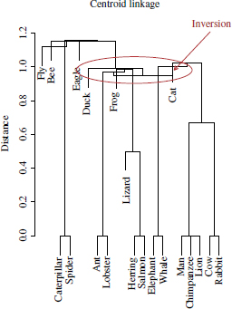
In the single linkage, the clusters with the closest members are merged. Such merging criterion is local, as the global cluster structure is ignored. As can be observed in the dendogram of Figure 2.1(a), the single linkage usually results in large clusters and may lead to erroneous splits of one cluster if two or more clusters are close to each other, specially if the clusters show different pattern densities (in this case, the pairwise distances in the low-density cluster may be larger than the distance between the two clusters). On the other hand, the complete link criterion merges two clusters according to the most distant objects. This criterion overcomes the problem of large clusters obtained by the single linkage. However, the complete link criterion is sensitive to outliers. If a cluster is merged to an outlier at a certain iteration, its inter-cluster distances will become considerably larger at the next iteration. This is due to the presence of the outlier pattern. This fact may prevent merging the cluster to other members of the same cluster in further iterations. A good compromise seems to be the average linkage criterion. It merges two clusters according to the average pairwise distances between their respective members. Finally, in the centroid linkage criterion the distance between two clusters is calculated as the distance between the centroid elements. One important characteristic of the centroid linkage method is that the cluster distances do not show increasing monotony with increasing iterations, in contrast to the single, complete, and average criteria. As an example, consider three globular, equally sized clusters, spatially arranged so that their centroids occupy the vertices of an approximately equilateral triangle, . The distance of the first two clusters, say C_a and C_b (edge ), is only marginally inferior to the length of the other two edges in the triangle, so that the clusters C_a and C_b are merged at iteration t. The centroid of the new cluster will be then placed in the middle point of the edge . The centroid of the third cluster corresponds to the third vertex. Thus, new distance between the new cluster C_ab and C_c, merged at iteration t + 1, corresponds to the height of the triangle, , which is smaller than the distance between the clusters C_a and C_b merged in the previous iteration. This non-monotonic distance effect is clearly patent in the new dendogram plot. It can be observed how mergings at a certain iteration can occur at a lower dissimilarity level than a previous iteration. Such effect is also known as dendogram inversion.

2.4.1.2. Divisive algorithms

Divisive algorithms build the cluster hierarchy in a top-down approach, starting at the top level, where all the patterns are enclosed in a unique cluster, and successively splitting clusters until each pattern is found in a singleton cluster. A greedy divisive algorithm requires the evaluation of all 2^|C|−1 − 1 possible divisions of the cluster C into two subclusters (initially, |C| = n). However, Smith et al. proposed an alternative algorithm, called divisive analysis (DiANA), which avoids the inspection of all possible cluster partitions. The algorithm is described as follows:

1. Start with all objects in a unique cluster, C_g.

2. Select the cluster C′ with the highest diameter (distance between the most distance objects inside the cluster). Initially, start with the cluster C_g containing all patterns in the dataset, i.e. C′(t = 0) = C_g.

3. For each object in C′, calculate its average distance to all other objects in the cluster.

4. Select the pattern with the highest average distance in C′. This pattern originates into a new cluster C″ and is thus removed from C′.

5. For each one of the remaining objects, x_i ∈ C′, calculate the average distance to the rest of objects in C′ and C″. Let this average distances be denoted as d_avg(x_i,C′) and d_avg(x_i, C″). If d_avg(x_i, C′)> d_avg(x_i, C″), the pattern has more affinity to the new formed cluster. Select the pattern whose affinity to C″ is the highest in comparison to C′.

[2.1]

Remove from C′ and attach to C″.

6.Repeat Step 5 until no object in C′ can be found such that davg(x_i,C′)> d_avg(x_i,C″). At this point, the partition of the cluster C is finished. Record the resulting clusters C′ and C″ into the corresponding dendogram level.

7. Stop if each data pattern is in its own cluster (the bottom hierarchy level is reached). Otherwise, repeat from Step 2 to evaluate the subsequent cluster to be partitioned.

2.4.2. Model-based clustering

In model-based clustering, it is assumed that the data are drawn from a probabilistic model, λ, with parameters θ. Thus, the estimation of the model parameters θ is a crucial step for identifying the underlying clusters. A typical example of model-based clustering is the expectation maximization (EM) algorithm.

2.4.2.1. The expectation maximization (EM) algorithm

As mentioned above, the EM algorithm [DEM 77, NIG 99, MAC 08] is based on the assumption that the dataset = {x₁,x₂,…, x_N} is drawn from an underlying probability distribution, with a probability density function p(X|θ). The objective of the EM algorithm is to provide an estimation of the parameter vector that maximizes the log-likelihood function

[2.2]

In a simple univariate Gaussian distribution, θ may be a vector of the mean and variance, θ = [μ, σ²]. An analytical solution to the maximum log-likelihood problem can be directly found by taking derivatives of equation [2.2] with respect to μ and σ. However, for more complex problems, an analytical expression may not be possible. In such cases, the EM algorithm performs an iterative search for the numerical solution of [2.2].

Typically, an additional unobserved variable vector Z is introduced. The introduction of this variable allows us to simplify the mathematical analysis to derive the EM updating equations

[2.3]

where z denotes a particular value of the variable vector Z. Let θ^(t) denote the guess of the parameters θ at iteration t. The derivation of the EM formulation follows the Jensen’s inequality

[2.4]

with constants λ_i ≤ 1, such that ∑_iλ_i = 1. At iteration t, the parameters θ^(t) are known. Thus, the constants λ_i can be defined as follows:

[2.5]

with ∑_ip(z|X, θ^(t)) = 1. These constants can be introduced in the log-likelihood formulation (equation [2.2]) as follows:

[2.6]

Thus, by applying Jensen’s inequality, it yields

[2.7]

Moreover, it can be shown that the log-likelihood equals equation [2.7] for θ = θ^(t). Thus, equation [2.7] is a lower bound of the log-likelihood to be maximized, and equals this likelihood for θ = θ^(t). This observation is key for the definition of an EM iteration. If a value θ(^t+1) is found to increase the value of equation [2.7], it will necessarily result in an increment of the log-likelihood value. The maximization objective can be thus reformulated as

[2.8]

At iteration t+1, the last term in equation [2.8] is a constant factor with respect to θ. Thus, this term can be discarded in the maximization formulation, which can be rewritten as

[2.9]

Thus, the objective of the EM algorithm is the maximization of the expectation of log p(X,z|θ) over the current distribution of Z values given X under θ^(t). Typically, a definition of the variable vector Z is used so that each z realization can be calculated from the current estimate of the parameters, θ(t). The iteration (t + 1) of the EM algorithm consists of two alternating steps:

1. E-step: determine the expectation . In practice, it requires the calculation of the probabilities p(z|X,θ^(t)) given the data and the previous parameter vector estimate θ^(t).

2. M-step: find the current estimation θ^(t+1) by maximising the expectation:

[2.10]

An example of the EM algorithm for estimating the parameters of a mixture of Gaussians is described in the following.

2.4.2.1.1. Example: mixtures of Gaussians

For a mixture of Gaussians with M components, G = {g₁,g₂,…,g_M}, the random variable vector Z is composed of N components, , where z_i ∈ [1,…,M] denotes the Gaussian component of the corresponding data element x_i. The parameter vector θ is thus composed of the Gaussians means and variances (μ, ∑), as well as their marginal probabilities p(g). Thus, θ is composed of M components, (θ₁,…, θ_M) for the M Gaussians, with θ_m = (μ_m, ∑_m,p(g_m)). The expectation in equation can be formulated as

[2.11]

After some manipulations, a more simple expression can be derived for equation [2.11] as follows:

[2.12]

where p(z_i = m) denotes the probability of the mth Gaussian component, p(g_m).

In the E-step, the first part of the expectation in equation [2.12], p(z_i = m|x_i,θ^(t)) can be calculated given the previous estimation of the parameters θ^(t):

[2.13]

After the calculation of the probabilities p(z_i = m|x_i,θ^(t) the Maximization of the expectation performed the M step, b taking the partial derivatives of equation [2.12] with respec to the parameters θ and setting their values to 0.

[2.14]

By considering the partial derivatives with respect to the individual components in θ (μ, σ and p(g)), the following solutions yield for μ^(t+1), ∑^(t+1) and p(g)^(t+1):

[2.15]

[2.16]

[2.17]

The E- and M-steps are iterated until the parameter vector θ^(t+1) remains unaltered with respect to the vector in the previous iteration, θ^(t) In this convergence state, a “soft” clustering solution is provided by the probabilities p(z_i = j|x_i,θM). However, a hard solution can be easily obtained by selecting the values of z_i which maximize these probabilities. The EM algorithm is considered as a generic modality of the k-means algorithm. In fact, both E- and M- steps are closely related to the k-means adaptation steps. The E-step recalculates the membership probabilities p(z_i|x_i), given the previous parameter estimate (means and covariances). This step can be viewed of as a soft version of the pattern reallocation in the Voronoi cells of the respective means in k-means. Finally, the recalculation of the means in k-means correspond to the update of the θ^(t+1) in the M-step.

2.4.3. Partitional competitive models

Competitive models aim at discovering a set of reference prototypes, = {p₁,p₂,…,p_n} with coordinates {ω₁, ω₂, …,ω_d}, which optimally represent the data distribution .

2.4.3.1. K-means

In general terms, assuming that the elements of are drawn from a certain probability distribution, P(x), the k-means [ART 06,BAR 00,HAR 05] objective is to find the values of the prototype vectors to minimize the error in

[2.18]

where _i is the Voronoi cell associated with the reference vector p_i, i.e. the region of points in ^D that are closer to p_i than to any other reference vector in :

[2.19]

If the probability distribution of the data, P(x), is not known a priori, but only a discrete set of data points = {x₁,X₂,…,x_N} is available, the error surface in equation [2.18] can be reformulated as

[2.20]

In the k-means algorithm, the search for the optimum weights of the prototypes is performed iteratively through a stochastic gradient descent on the error surface. At iteration t, the contribution of the data element x(t) to the update of the prototype weights is thus given by

[2.21]

where x(t) denotes the data point visited at time t, ∈(t) is the step size parameter that controls the adaptation rate, and δ_ii is the Kronecker delta function defined as follows:

[2.22]

Hence, the function δ_iix(t)) deactivates any possible contribution of elements that lie outside the Voronoi region of p_i. Owing to this “hard decision,” the fc-means algorithm is casted as a hard competitive model, which means that only points for which p_i is found to be the “winning prototype” account for the update of the prototype weights.

It should also be noted that, after each update of the prototype weights, the Voronoi region of the prototype p_i is recalculated. Moreover, the parameter ∈(t) is not constant, but obeys a decaying pattern:

[2.23]

where n(t) is the number of visited data elements that have contributed to the update of the weights of p_i up to the current iteration t.

As it can be demonstrated, the prototypes’ weight locations converge asymptotically to the mean expected value of their respective Voronoi cells:

[2.24]

or equivalently, for a discrete dataset

[2.25]

A batch implementation of the k-means clustering algorithm can be described as follows:

1. Initialize the set of prototypes with k elements,

[2.26]

whose weights or cooordinates w_i are randomly chosen according to p(x) or selected by the user.

2. For each iteration t, build a set of clusters around the respective prototypes:

[2.27]

in such a way that each cluster is composed by the data points belonging to the Voronoi cell of the winning prototype

[2.28]

3. Re-calculate the prototype weights or coordinates to coincide with the most central point of the Voronoi cell:

[2.29]

4.Calculate the error at iteration t, E^(t), according to equation [2.20].

5.Calculate the decrement of the error E at iteration t with respect to t − 1:

[2.30]

6. Stop if the error difference Δ_E is lower than a specified value, (a convergence status is reached), or the maximum number of iterations is reached. Otherwise, continue from Step 2.

Figure 2.4 shows an example of the clustering solution obtained by the k-means algorithm on a mixture of five Gaussians with two different random initialization. As can be observed, the extracted clusters depend on the choice for the initial prototypes. An inappropriate initialization may lead to solutions far from the optimum (Figure 2.4(a)).

2.4.3.1.1. Advantages and drawbacks

One of the advantages of k-means is the fast convergence and thus the low computational cost of the algorithm [HAR 05]. However, the main limitation associated with the k-means algorithm may converge to a local optimum, depending on the choice of the initial prototypes. This problem is commonly addressed through multiple algorithm calls with different random initializations in a trial-and-error approach. The solution that provides the minimum sum of squared errors is selected.

Another limitation is associated with the sum of squared errors objective function. Patterns with large distances may considerably attract the cluster centers toward them. Consequently, the algorithm shows a high sensitivity to outliers.

A third limitation of k-means is the shape and size of clusters that can be detected. As the algorithm divides the dataset into Voronoi regions, the k-means algorithm extracts convex (globular) clusters. However, it may fail to identify other cluster shapes or clusters of non-homogeneous sizes, specially if those clusters lie close to each other.

Finally, the k-means algorithm requires the number of clusters k to be a priori determined. The correct identification of the optimal number of clusters existing in a dataset can be achieved through the evaluation of the cluster partitions obtained from multiple runs of the clustering algorithm with different values of k; see Chapter 6 for other possibilities.

2.4.3.2. Neural gas

As described in the preceding paragraphs, the weight adaptation of each prototype p_i by the k-means algorithm is only affected by the data points whose winning prototype is p_i. In contrast, in the neural gas approach [COT 00,FRI 95, FYF 06], each visited data point, x_j ∈ , has a certain impact on the adaptation of the weights for all prototypes, on a “rank order” basis (equation [2.31]):

[2.31]

As can be noted, the main difference with respect to the weight adjustment in k-means (equation [2.21]) is the substitution of the delta function by an exponentially decaying function (h_λ). Basically, this new function determines the relative (soft) importance of each presented data point at iteration t, x(t), for the adaptation of the prototype p_i:

[2.32]

where k_i indicates the rank order of the prototype p_i from all prototypes in with respect to the data point x(t) under consideration. In other words, k_i is the number of prototypes closer to x(t) than p_i. For example, the closest prototype is assigned a rank order k = 0, and thus, h_λ(k_i(x(t))) = 1; Analogously, the next, second, third, etc., closest prototypes up to the farthest one are assigned rank values k = 1,2…, k − 1. The λ parameter, λ∈ [0,1], controls the decay rate of the h_λ function, and thus, the “softness” of the neural gas model. For example, if λ→ 0, the function h_λ is equivalent to the Kronecker delta δ_ii and thus the resulting model becomes analogous to the k-means algorithm.

It can be shown that the adaptation rule in equation [2.31] responds to a gradient descent optimum search on the error function in equation [2.33]:

[2.33]

For a discrete dataset, equation [2.33] is equivalent to [2.34]:

[2.34]

The normalization factor C(λ) in both equations [2.33] and [2.34] is a constant value that only depends on λ:

[2.35]

2.4.3.2.1. Advantages and drawbacks

The main advantage of the neural gas with respect to the k-means algorithm is the robustness with respect to the initialization. The neural gas can be viewed as a generalized version of Kohonen maps which applies to any topology. However, the algorithm requires, besides the number of clusters k, the specification of other parameters, such as the adaptation rate and the neighbor functions.

2.4.3.3. Partitioning around Medoids (PAM)

The Partitioning around Medoids (PAM) algorithm, proposed by Rousseau [LEO 05] is an alternative to the k-means algorithm based on medoid prototypes. In a similar way as k-means, the PAM algorithm aims at discovering a set of k representative objects that are more centrally located in the clusters. However, PAM differs from the k-means in several ways:

1. PAM searches for a set of k-medoid prototypes instead of k-centers. Centers (or centroids) are vectors located in the exact cluster “center of masses” and do not necessarily coincide with an object in the dataset. In contrast, medoids correspond to the objects in a dataset closer to the cluster means.

2. The objective function minimized by the PAM algorithm is the total sum of distances, instead of the sum of squared errors in k-means.

3. The PAM algorithm may be used with any arbitrary distance function. It also accepts the matrix of data dissimilarities as input instead of the dataset coordinates.

The search for the minimum sum of distances is performed in two main steps: build and swap.

2.4.3.3.1. Build step

This step performs a sequential search for an appropriate initial set of medoids , which are more “centrally located” [LEO 05] in the dataset:

1. Select the object ⁽⁰⁾ with the minimum sum of distances to the rest of elements in the dataset. Initially (at iteration t = 0), the set of prototypes is composed by the object x⁽⁰⁾.

[2.36]

[2.37]

2. Select a candidate object outside the current prototype set, x_i ∉ . A quality score S(x_i) is computed for the selected object. It measures the distances between all other objects and x_i in relation to their distances to :

[2.38]

[2.39]

where d_min(x_k,) denotes the distance of x_k to the closest prototype in .

3. Repeat Step 2 to compute the scores S(x_i) for all candidate objects outside . At iteration t, select the object (t) with the maximum score S(x_i) and update the set of prototypes with :

[2.40]

[2.41]

4. Repeat Steps 2 and 3 while incrementally adding new prototypes to until k prototypes are found, i.e. || = k.

2.4.3.3.2. Swap phase

In the second phase of the algorithm, all possible exchanges, or swaps between the prototypes and the rest of objects, are evaluated to minimize the objective function. If a swap (x_i ∈ ↔ x_j ∈ ) is carried out, the object x_i is removed from the set of prototypes in favor of x_j, which is attached to .

1. For each possible swap in the form (x_i ∈ ↔ x_j ∉ ), the “goodness” of the swap is evaluated by a score T(x_i,x_j), calculated as the sum of individual contributions C_i,j,k for all other objects, x_k ∉ P:

[2.42]

[2.43]

where d_min(x_k, ) denotes the minimum distance of x_i to any of the objects in .

2. Select the pair with the minimum score T(x_i, x_j ):

[2.44]

3. Stop if T. Otherwise, carry out the swap and repeat from Step 1 to evaluate further potential swaps.

2.4.3.3.3. Advantages and drawbacks

In comparison to the k-means algorithm, the PAM reaches the global optimum regardless of the medoids initialization. However, this is achieved at the expense of higher computational cost. Moreover, since the optimum criterion is to minimize the total sum of distances instead of squared distances, the PAM algorithm is more robust against outliers. As in k-means, the PAM extracts Voronoi regions around the medoid objects and may thus fail to detect non-convex clusters.

2.4.3.4. Self-organizing maps

The self-organizing map (SOM) is a popular tool for exploratory data analysis, devised by Teuvo Kohonen [KOH 01, KOH 90, VES 00]. Kohonen’s model belongs to the category of algorithmic approaches inspired by biological processes. The SOM principle shows a direct analogy with the logical perception of different input stimuli by the human brain. Numerous studies in the field of neurobiology have ascertained how the different sensorial stimuli, in the form of multi-dimensional signals, are projected in specific regions of the cerebral cortex. It has been observed that, within each region, the information is mapped into certain topological structures, which are typically configured in linear of planar (bi-dimensional) maps. This peculiar characteristic of the brain is commonly referred to as the “topology preserving” property and was exploited by Kohonen in the SOM model.

The basic SOM model can be observed in Figure 2.5. In contrast to the previous generative algorithms, the set of prototypes is organized in a topology (ordered map) of a lower dimensionality m than the input dataset. Following the typical structures in the brain, such maps are usually one or two dimensional. The SOM prototypes can thus be considered as the nodes in the ordered map, also referred to as neurons. In compliance with the topology preserving condition, the ordering of the nodes in the map (Kohonen layer) is fixed at all stages of the algorithm. In addition, each node p_i is associated with a weight vector w_i ∈ ⁿ that corresponds to any point in the input data space. In a learning phase, the nodes’ weights are iteratively updated, until the final prototype weights reflect the input data distribution. In other words, the distribution of the final prototype weights in the input layer is the most representative for the input data distribution.

Initially, the prototype weights are assigned random values. At each iteration t, an input vector from the dataset is selected x(t). The prototype p_k in the Kohonen layer with the closest weight vector to x(t) is then selected as the winning prototype. In SOM models, the winning prototype is referred to as the best matching unit (BMU).

The weight vectors of the BMU (w_k) and its neighbors are displaced toward the direction of the input element x(t), using the weight update rule:

[2.45]

where α(t) denotes the SOM learning rate, which decreases monotonically with each iteration. h_k,i is a spatial neighborhood function that determines the degree to which the input vector x(t) “attracts” the BMU’s neighbor neurons in the Kohonen layer. At an attempt to emulate the biological lateral interaction between adjacent neurons, a Gaussian function is frequently selected for the neighborhood function h_k,i:

[2.46]

where r_i and r_k denote m-dimensional vectors with the spatial coordinates of the nodes k (BMU) and i in the map. As with the learning rate, the standard deviation σ in equation [2.46] is also a decreasing function with the number of iterations t. Thus, during the learning progress, the map becomes more “specialized” by increasing the spatial resolution of the neighborhood function.

The steps of the SOM learning algorithm are as follows:

1. Given an input finite dataset , and a selected topology, initialize the codebook of prototypes (t = 0) = {p₁,p₂,…,P_k}. If a random initialization is selected, each jth prototype variable takes k random values uniformly distributed in the original range of the corresponding variable in .

2. Select an input pattern x(t) from the finite dataset . Calculate the distance (typically, the Euclidean distance metric is used) of the input pattern to all prototypes in . The winner prototype — BMU — is identified as :

[2.47]

3. Update the prototype weights of the BMU and its spatial node neighbors in the map toward the direction of the pattern x(t), according to the weight update rule (equation [2.45]).

4. Stop if the maximum number of iterations is not exceeded (t < maxiter). Otherwise repeat from Step 2 with t = t + 1.

To obtain final prototype weights which are good representatives of the input data distribution, an adequate choice for the maximum number of iterations maxiter is a multiple of the input dataset cardinality maxiter := N · ||, so that each data element x_i ∈ D is exactly presented N times to the SOM learning algorithm.

The multiplier factor N is also referred to as the number of cycles or epochs. Figure 2.6 shows an example of the prototype weights adaptation (input layer) on the mixture of five Gaussians over 100,000 iteration. Grey dots depict the nodes distribution at different stages of the algorithms, whereas black dots depict the dinal convergence positions. Figure 2.7 shows another example using a 10x10 sheet topology, after the initialization (Figure 2.7(a)) and after 10,000 iterations (Figure 2.7(b)). The corresponding U-matrices are also depicted (Figures 2.7(c) and 2.7(d)).

2.4.3.4.1. Advantages and drawbacks

The main advantage of Kohonen SOMs relies on their capability to fit any type of distribution. The SOMs for clustering have several possibilities. If the number of clusters, k, is known, a topology (e.g. linear) with k nodes can be selected. At the convergence state, a cluster can be considered as the patterns which share the same BMU unit. Alternatively, a larger topology may be selected in combination with any k-clustering approach to partition the nodes in the Kohonen layer. Finally, if the number of clusters is unknown, the SOM can be used as a visualization tool. The task to recognize the number of clusters is left to the users who analyze the so-called U-matrix (as in Figure 2.7(d)).

However, this task has some limitations. For example, although the SOM does not require the number of clusters, the final distribution of nodes — as well as the U-Matrix — also depends on the topology and the map size, which has to be determined beforehand. It is also known that, to obtain accurate results, large maps are usually required, which increases the algorithm complexity. Finally, the analysis of the U-matrix to determine the number of clusters has the limitations of a subjective task. Such decision may vary from user to user, specially for close clusters or for large ks.

2.4.4. Density-based clustering

In contrast to the classical hierarchical and divisive approaches, in which clusters arise based on the objects’ distances, density algorithms build the clusters based on a density concept [EST 96, SAN 98]. This means that clusters are located in regions with roughly homogeneous densities.

The most popular approach to density clustering is probably the Density-Based Algorithm for Discovering Clusters in Large Spatial Databases with Noise (DBSCAN), proposed in [EST 96]. The density concept in the DBSCAN algorithm is indicated by the input parameters (minpts and eps), which denote the minimum number of points to be enclosed in a neighborhood of radius eps, respectively.

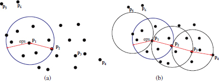
In the DBSCAN algorithm, two types of objects are distinguished: cluster and noise. To formulate the notion of cluster in DBSCAN, the concepts of direct density reachability and density connection were introduced, which are illustrated in Figure 2.8.

2.4.4.1. Direct density reachability

Figure 2.8(a) shows an hypothetical spatial dataset, as well as the ∈ neighborhood of the point p₁. Moreover, assuming a particular value of minpts = 4, the point p₁ is said to be a core point, and all points in its ∈ neighborhood, such as p₂, are density reachable from p₁.

2.4.4.2. Density reachability

Figure 2.8(b) shows the concept of density reachability and density connection with respect to minpts and ∈. For example, p₃ is not directly reachable from p₁ since it falls outside the eps neighborhood of p₁. However, it is density reachable from p₁, because it is possible to find one or more points pi directly reachable from p_i−1, starting at p₃ and ending at p₁. In this particular case, p₃ is density reachable from p₁ because it is directly reachable from p₂, which in turn is directly reachable from p₁. Likewise, we can argue that p₄ is also density reachable from p₁ through p₃ and p₂.

2.4.4.3. Density connection

Furthermore, p₃ and p₁ are also said to be density connected, because there exists at least one intermediate point (in this case p₂), from which both p₁ and p₃ are density reachable. In addition, p₄ is density connected to p₁ through p₃ or p₂. It should be noted that density connection does always imply density reachability. For example, in Figure 2.8(b), although p₁ is density connected to p₄, it is not reachable from p₄, since p₄ is not a core point.

2.4.4.4. Border points

In Figure 2.8(b), p₄ is of a different type to p₃, p₂, and p₁. The latter objects are called core points because we can always find a number of points greater than minpts in their neighborhood. In contrast, the point p₄ is called a border point because its neighborhood contains less than minpts = 4.

2.4.4.5. Noise points

It should be noted that the concept of border point implies that the point is density reachable from at least one point, as with p₄. In contrast, the points p₅ and p₆, which also contain less than minpts in their eps neighborhoods, are not density reachable from any point in the dataset. These are thus located in a non-dense area and are treated as noise points.

2.4.4.6. DBSCAN algorithm

Each cluster found by the DBSCAN algorithm is thus composed of a set of density connected points. Assume denotes the input dataset, and the sets of unclassified and noise points, respectively, and the final set of clusters, the DBSCAN algorithm can be described in the following steps:

1. Initially, the set of unclassified objects is equal to the input dataset, and the set of noise patterns is the empty set:

[2.48]

2. Select a non-classified object x_i ∈ around which a new potential cluster is to be build, _i:

[2.49]

3. Calculate the set of data elements with lower distance to x_i than eps.

4. If |S| < minpts, x_i is not a core object. The candidate cluster C_i is discarded.

[2.50]

Go to Step 1 to explore for other initial objects.

5. If |S| ≥ minpts, all objects in |S| are direct density reachable from x_i . The new cluster C_i will thus contain at least the objects in . Remove the objects from the set of unclassified patterns and go to Step 5

[2.51]

6. Select a random object from , x′, and calculate the set of points ′ which are less or equal distance than eps from x′. Remove x′ from the set S of points to be further visited, adding x′ to the growing cluster C_i:

[2.52]

7. If |′| > minpts, the chain of density reachable points from x can be extended by exploring the elements of S′. Thus, add these elements to the set of points to be visited and remove them from the set of unclassified objects:

[2.53]

8. Repeat Steps 6 and 7 until = θ. This means that the chain of density reachable objects from x has been completed, and thus, no more points need to be further visited. Add the new cluster C_i to the set of clusters:

[2.54]

9. Repeat from Step 1 to search for more possible clusters, until no further data elements can be found in with more than minpts in their eps neighborhoods. In this case, the remaining unclassified objects in compose the set of noise patterns ( = ).

2.4.4.6.1. Advantages and drawbacks

In contrast to the previous algorithms, the DBSCAN algorithm is based on density parameters instead of distances. Thereby, DBSCAN is not only able to extract globular clusters but also can identify cluster of different shapes and/or sizes. One limitation of the DBSCAN algorithm is, however, related to the a-priory determination of the minimum cluster density to be extracted (input parameters minpts and eps).

2.4.5. Graph-based clustering

In a graph-based clustering, the data objects are arranged as vertices of a graph G(,), with a set of edges E. Different clustering algorithms exist based on graphs, such as Metis, Hmetis [KAR 98], or mincut [FEN 09]. In this book, the pole-based overlapping algorithm has been considered. This approach extracts the final clusters without any a priori parameter.

2.4.5.1. Pole-based overlapping clustering

The pole-based overlapping clustering (PoBOC) is an overlapping, graph-based clustering technique proposed by Cleizou [CLE 04a,CLE 04b]. The algorithm takes the matrix of object dissimilarities as single input and builds the output clusters in four main steps: (i) definition of dissimilarity graph, (ii) construction of poles, (iii) pole restriction, and (iv) affectation of objects to poles.

2.4.5.1.1. Definition of a dissimilarity graph

Let denote the set of objects in the dataset and the dissimilarity matrix, computed over . The mean distance of an object x to all other objects in , d_mean(x,), is formulated as:

[2.55]

The dissimilarity graph G(,,) is then specified by (i) the dissimilarity matrix and (ii) the data points or vertices, , and a set of edges between all pairs of vertices (x_i, x_j) corresponding to mutual neighbor points.

DEFINITION 2.1.– Neighborhood of a point x. The neighborhood of a point , denoted by N(x) is composed of all points of whose dissimilarity to the point is smaller than the mean distance of the object x to all other objects in (d_mean(x; )):

[2.56]

DEFINITION 2.2.– Mutual neighborhoods. Two points (x_i, x_j) are mutual neighbors, and thus connected by an edge in , if each one belongs to the neighborhood of the other:

[2.57]

2.4.5.1.2. Pole construction

This procedure builds incrementally a set of poles = {P₁, P₂ …, P_k} over based on the dissimilarity matrix and the dissimilarity graph G(, , ). Let denote the cumulated set of objects that belong to any of the extracted poles up to the current state (initially the empty set).

The poles are grown from initial points i, which are the points with maximum mean distance to the cumulated set of poles . Initially, the object ₀with maximum distance to is selected:

[2.58]

Each P_i pole is then grown from the corresponding initial object

[2.59]

in such a way that all the pole members are mutual neighbors of each other. This is implemented in the build-pole procedure:

The selection of the initial object _i and the construction of the corresponding pole Pi are iteratively repeated until all objects in the dataset are contained in any of the poles, = , or no initial object can be found which is sufficiently distant from the set of poles.

2.4.5.1.3. Pole restriction

After the pole construction, overlapping objects may be obtained. These are objects that simultaneously belong to two or more poles. Overlapping compose the residual set . The pole restriction procedure removes the residual objects from the original poles, resulting in a new set of reduced, non-overlapping poles .

2.4.6. Affectation stage

The set of residual objects obtained at the pole restriction stage require some post-processing strategy to be re-allocated into one or more of the restricted poles. This re-allocation of objects in PoBOC is called affectation. First, the membership of each object x to each -restricted pole, u(x, ), is computed as:

[2.60]

Next, the objects are affected to one or more poles. In a single-affectation approach, each object x is assigned to the pole maximizing the membership u(x,_j). In a multi-affectation approach, the object is affected to the poles whose memberships are greater than some reference values given by a linear approximation on the set of object memberships, sorted in decreasing order.

2.4.6.1. Advantages and drawbacks

The main advantage of the PoBOC algorithm is that no-apriori knowledge is required to obtain the cluster solution. The algorithm is able to extract the clusters with no input parameter. However, one limitation of PoBOC is related to the internal parameter used by the algorithm to build the dissimilarity graph, namely, the average object distances. Due to this internal parameter, PoBOC may fail to detect clusters in hierarchies or with non-homogeneneous inter-cluster distances. A solution to this limitation is provided in Chapter 5.

2.5. Applications of cluster analysis

One outstanding characteristic of cluster analysis is the multi-disciplinary application of the clustering techniques. This fact is primarily related to the diverse nature of the data which can be subjected to exploratory analysis. The only requisite for the input dataset is the multivariate formulation of the entities to be clustered, in terms of a set of properties or measurements (variables or features).

2.5.1. Image segmentation

Image segmentation techniques divide an input image into a set of non-overlapping regions that are roughly homogeneous based on features of interest, such as texture, color, intensity, and sometimes, the pixels’ positions [LO 07, OUY 09]. Image segmentation is used for multiple purposes, typically as a pre-processing component that allows us to recognize small segments to be posteriorly labeled or classified. Different approaches for image segmentation can be encountered in the image processing and computer vision literature, including watershed techniques using mathematical morphology [YE 09], edge finding [YAN 09], region growing [MAN 00], artificial neural networks [MUK 08], thresholding, and clustering [DES 09]. According to Jain, thresholding is a particular case of clustering in a binary form (using only two target clusters).

One example application of image segmentation is for medical images. Clustering — among the rest of techniques — can be used to analyze different image modalities: magnetic resonance images (MRI) of the brain, computed tomographies (CT), chest radiographies or digital mammographies, among others, to distinguish different types of tissue or localize suspicious elements — tumors — for posterior classification or diagnosis.

A second example of segmentation using clustering is shown in Figure 2.9. The plots show two-digital slide brain images (a,d), segmented using the k-means (b,e), and EM (c, f) algorithms. Among the output clusters, different brain tissues can be distinguished (white mass, gray mass, and cerebrospinal fluid).

Another application of clustering-based image segmentation is for content-based image retrieval in which users query a database of images at the level of objects, such as traffic signs, cars, faces, and buildings. The objective of segmentation for content-based image retrieval is to identify such regions in the image that possibly correspond to objects or parts of them [PAR 07]. Among the different segmentation modalities for object-based image retrieval, cluster analysis can be particularly applied to the so-called ‘Blobworld’ representation. The blobs are defined as the segmented regions, typically extracted via clustering, where the segmentation features (color, texture, etc.) remain approximately homogeneous. Each blob is finally represented in terms of its intrinsic descriptors, such as the dominant color and mean texture. When the users want to initiate the search for a particular object, they are asked to present an image somehow related to the object of interest. The segmentation algorithm is then applied to the query image, and its output is presented back to the user, together with the set of descriptors associated with the extracted blobs. The user is now able to specify the blob or a combination of them to be retrieved from the database or refine the query by some relevant descriptor values. It should be noted that, when the query response is obtained, the user has access to a complete blob information related to the retrieved segmented images, which also allows for more refined searches, in comparison with other image retrieval strategies. The blobword representation was introduced by [CAR 02], who used the EM algorithm to segment images based on the aforementioned features (color, texture, and spatial characteristics). Finally, clustering analysis has also been recently applied to face recognition, even though clustering is not a common practice in segmentation for face detection nor face feature extraction. Nonetheless, in [CHE 09], a hierarchical agglomerative clustering algorithm was applied in conjunction with a statistical classifier (support vector machines (SVMs)) to improve the efficiency and effectiveness of the recognition task. In particular, the agglomerative algorithm was used to group similar faces in the training set, followed by a two-step SVM using Bayesian modeling of face differences. Thereby, a manageable number of SVM hyperplanes was attained, despite the large number of faces (classes) in the database.

2.5.2. Molecular biology

During the past decade, the analysis of deoxyribonucleic acid (DNA) microarray data, which encodes the expression levels of a number of genes in cells from different tissues or organisms, has become a major common field of study in the areas of molecular biology and computer science.

2.5.2.1. Biological considerations

Gene expression or DNA microarray data is obtained by means of DNA microarray assays in which the activity of thousands of genes is monitored simultaneously [THE 09].

In a microarray experiment [CHU 02], a DNA microarray (DNA chip) is prepared. Basically, a DNA chip is a substrate slide, like glass or nylon. It contains an array of spots, pre-filled with oligonucleotide probes for a series of genes to be monitored. First, two cell samples are extracted from different populations to compare. For example, if the goal is to analyze the expression of responsible genes for a certain tumor, it is common to select a sample from a tumor cell and a second one from a normal cell. The mRNA from both cells is then extracted and marked with two different fluorescent dyes, typically blue and red. Next, the microarray chip is flooded with the mixed mRNAs, which hybridize with the spot nucleotides. By analyzing the microarray outcomes under a laser microscope with different wavelengths — read and green lights — two digital images are generated, where the spots hybridized with each colored mRNA can be detected. Finally, for each spot, the relative abundance of the gene expression in the first population (e.g. tumor cells) with respect to the second (e.g. normal cells) can be measured by,

[2.61]

Typically, microarray data are arranged as a n by m matrix of expression levels, S, in which rows are related to genes and columns to different experimental samples (also called conditions) (Table 2.2):

The elements s_ij are real values denoting the relative abundance of the gene’s mRNA i under condition (sample) j [BRO 99a].

The fundamental objectives of DNA microarray data analysis are to identify genes involved in certain biological processes, such as diseases, and specially, cancers, or to classify/identify different types and subtypes of cancer tissues on the basis of the gene activity profiles in tumor cells [HAS 00,BRO 99b].

The advances in DNA microarray technologies have made possible to obtain gene expression measurements for thousands of genes. Last generation sequencing techniques have even succeeded in generating complete genomic sequences. As is commonly accepted, the human genome is composed of approximately 30,000 genes (cite in gene selection for microarray data). However, only small groups of genes are expected to participate in active cellular processes of interest. For example, around 57 genes have been found to be responsible for breast cancers and around 158 for pancreatic cancers. Given the huge amounts of gene expression measurements collected from DNA microarray experiments, clustering techniques have been broadly applied to the efficient analysis, organization, and understanding of microarray tables.

One of the first references for clustering microarray data was the paper by [EIS 98]. They illustrated the usefulness of hierarchical clustering schemes in grouping together genes with similar functions, applied to gene expression profiles in the budding yeast Saccharomyces cerevisiae. A graphical representation of the clustered data was also proposed as an intuitive tool to facilitate the interpretation of the clustering results. Tavauoie et al. [BAG 06] used partitional k-means to extract groups of functional genes from the budding yeast. In this case, the samples were obtained at 15 different time points corresponding to different phases of the cells’ cycles. SOMs have been also widely applied to DNA microarray data. For example, [TAM 99] used spherical SOMs (sSOMs) for clustering genes in mouse brain tumor cell lines (Figure 2.10).

The aforementioned contributions are examples of genebased clustering, where the objective is, exclusively, to find groups of genes that share similar properties through different samples. A high number of research works on DNA microarray data analysis can be circumscribed in this category, considered as the standard approach for gene expression data.

As mentioned earlier, a second purpose of microarray data analysis is to identify groups of samples that share similar gene expression patterns. This approach, called sample-based clustering, has gathered notably fewer contributions in comparison with gene-based clustering, specially due to the cost of microarray chips used in different experiments (samples). More recently, new gene clustering approaches have been implemented, which aim at clustering genes and samples (rows and columns of the gene expression matrix) simultaneously. These approaches are commonly referred to as subspace clustering or bi-clustering [CHE 00,GET 00].

2.5.3. Information retrieval and document clustering

The term information retrieval (IR) refers to the search of information in unstructured databases (typically collections of documents) [RIJ 79, MAN 08]. A canonical example is the search of documents from the World Wide Web (www) [WUL 97]. The interfaces and search tools to retrieve relevant documents from the Web upon a user query are called Web crawlers or Web search engines (Google, Yahoo, Altavista, etc.). Other classical applications of IR is the search for books in digital libraries [JON 07, CHU 99]. Essentially, the users query the document database by typing one or more keywords that define the topic of interest. Some Web search engines support more complex queries also with different logical operators AND, OR, etc. The IR system then tries to match the documents in the database against the query words and retrieve the set of documents ranked as more relevant for the user’s query.

More recently, due to the progress of automatic speech recognition (ASR) [RAB 93], the vector-based call routing approach has emerged as a new, speech-based modality of IR for call routing applications [CHU 99, SAL 71]. The goal is to redirect the user call to the most relevant module destination according to the caller utterance. The possible call destinations are modeled by “virtual documents” (created during training phases of the system) and the callers’ query utterances are transcribed to textual words by the ASR. Thus, the task is analogous to a classical IR problem and can be resolved using IR tools and procedures.

One of the main tasks performed by IR systems is the representation of documents and queries that allows us to quantify the semantic “similarities” between documents or between documents and queries. Typically, documents are represented on the basis of word descriptors. The set of term descriptors is known as vocabulary or lexicon W. It is commonly extracted through certain pre-processing steps applied to a collection of (training) documents. These are described in the following sections.

2.5.3.1. Document pre-processing

Typically, the pre-processing task is accomplished in three main steps: feature selection, stop-word filtering, and surface form reduction (word lemmatizing or stemming).

2.5.3.1.1. Word selection

The aim of feature selection is to reduce the dimensionality of the document space by identifying and removing uninformative, non-discriminative words, while retaining only the informative words. The main characteristic of uninformative words is their roughly uniform distribution over different document categories, in comparison with discriminative words. Word selection is usually addressed by ranking all words in the documents according to a certain relevance score and filtering out words that do not exceed a given relevance threshold. Some word scoring metrics are, for example, IDF, TFIDF, or mutual information [YAN 97,FOR 03, GUY 03].

Owing to the “noisy” character of irrelevant words, not only a dimensionality reduction is attained by means of word selection, but also the effectiveness of IR systems and document classification can be substantially increased.

Another strategy to reduce the dimensionality of the document space is to feature extraction. A common approach applied to document collections is known as “latent semantic analysis (LSA)” [LAN 98, DEE 90]. Basically, LSA performs a singular vector decomposition (SVD) to the term document matrix. As a result, the initial word and document spaces are mapped into two new spaces of eigenvectors of lower dimensionality (S and D). The new dimension is determined by the non-zero eigenvalues in the matrix V. Feature transformation via latent semantic analysis can also help to remove the “noise” induced by words in the term document matrix due to certain lexical properties, namely, synonymy and polysemy. Finally, word feature clustering has been also applied as a feature extraction method for document classification [WUL 97].

2.5.3.1.2. Stop word filtering

In contrast to feature selection, stop word filtering is performed on the basis of manually pre-established lists, such as the SMART stop list [BLA 07, DRA 09]. Stop words are reportedly irrelevant for IR purposes as well as document clustering and classification, as they do not convey any semantic information to a document or text. Some examples of stop words are pronouns (He, etc.), prepositions (of, for, the), and, in natural language texts (such as the texts transcribed from speech by an ASR), words typical for spontaneous speech (eh, ehm, uh).

2.5.3.1.3. Word lemmatizing/stemming

This stage aims to reduce the normal, “surface” form of words into their “canonical” forms: stems or lemmas. The objective is to eliminate the morphological variability introduced by inflectional and/or derivative suffixes to retain the units of semantic meaning [POR 80,SCH 94]. According to different criteria, either word stemmers or lemmatizers can be applied to extract word stems or lemmas, respectively. A word stemmer removes any kind of inflectional and derivative suffixes from the surface word form to extract the word stem. This procedure can end up in a different lexical category (also referred to as part of speech (PoS)) with respect to the initial word (for example, workers → work). In contrast, a word lemmatizer eliminates only infectional suffixes from the surface form of the word, e.g. plurals of nouns are reduced to singular forms and conjugated forms of verbs are reduced to the infinitive form. The PoS tag of the initial word is thus preserved. Lemmas are also known as the “dictionary form” of words, since it is the form in which all entries in a dictionary are presented.

The vocabulary W is finally composed of all distinct lemmas or stems observed in the pre-processed documents.

2.5.3.2. Boolean model representation

In a Boolean model [KLE 00, LAS 09], each document in the collection can be viewed as a Boolean vector whose components denote the presence or absence of the lexicon terms in the document. For example, imagine a library application where the search is for books relevant to a topic. The document dataset might consist of the following book titles (documents): E.g. D1 = Data mining applications; D2 = Algorithms for clustering data; D3 = Clustering analysis; D4 = Clustering text documents; and D5= Algorithms for document clustering. If a word lemmatizer is applied and a unigram approach is selected, the resulting lexicon of terms, in alphabetical order, is {} = Algorithms, Analysis, Applications, Cluster, Data, Document, Mine, and Text. The Boolean representation of the set of documents can be observed in Table 2.2.

A Boolean query, , is then composed of terms and Boolean operators. The three standard Boolean operators are AND, OR and NOT. As an example, a possible query related to the previous example could be = [Clustering AND NOT Documents AND Algorithms]. The result is obtained by computing the bitwise logical AND between the terms t4 (Cluster) and t1 (Algorithm) and the Boolean negative of the term t6 (Document) (see Table 2.3).

As can be noted, the search result to the Boolean query is the document (book title) D2 (Algorithms for Clustering Data). In Boolean retrieval, all exact matches are typically returned to the user, although there have been proposals for improving the presentation of results by ranking the documents according to the frequency of the query terms in the documents.

2.5.3.3. Vector space model

In the so-called vector-model representation [SAL 75, STE 00, PRI 03], used in IR, and the close areas document clustering or classification, a collection of documents is typically arranged as a matrix and a query as a term vector Q:

[2.62]

The matrix is also commonly referred to as the document term matrix, in which rows represent documents in the collection and columns refer to the lexicon terms {}. These two dimensions of the matrix (documents and words) are also referred to as the document space and the word space, respectively.

In a vector space model, the retrieved documents are typically ranked on the basis of their relevance to the user’s query, which can be estimated by measuring the cosine similarity between their respective vectors (,[i]). It should be noted that the cosine similarity metric is equivalent to the dot product similarity (equation [2.63]), if both [i] and vectors are normalized to have unit lengths:

[2.63]

2.5.3.4. Term weighting

In a similar way as in Boolean retrieval, the entries d_ij of the document term matrix can be just set to “0” or “1”, denoting the presence of absence of the w_j word in the ith document in the collection. This Boolean notation can be also used for the query elements q_i. In such a case, the query is referred to as Boolean query, although this term should not be confused with the definition of Boolean queries used in Boolean retrieval models.

More sophisticated approaches apply term weighting methods to compute the scores d_ij and q_j, which denote the relative significance of each lexicon term w_j in the query and/or document vectors [SAL 88]. To estimate the importance of terms with respect to the document or query, a term weighting formulation consists typically of three different components.

2.5.3.4.1. Term frequency component

The basic idea behind the term frequency [RAM 00] component is that a term that occurs more often in a document is more important to describe the contents of the text. Different notations have been used in the IR literature for the term frequency component

[2.64]

[2.65]

[2.66]

where C(w_j, d_i) denotes the counts of occurrences of the w_j word in the document. The first formulation, TF_(a), is also referred to as the raw term frequency, while the second and third, TF_(b) and TF_(c), are referred to as the relative term frequency and augmented term frequency, respectively.

2.5.3.4.2. Collection frequency component

The collection frequency factor captures the “informativeness” of words with respect to the complete collection of documents. The main assumption is that words that tend to occur in many documents are in general less discriminative for such documents than words occurring in a small number of documents and vice-versa. Different metrics have been proposed for the collection frequency component such as the Inverse document frequency (IDF) and the residual inverse document frequency (RIDF).

The most popular metric for the collection frequency component is the IDE [SAL 88], which measures, the inverse of the ratio of documents in which a word occur, with respect to the whole number of documents in the collection.

Two different formulations have been proposed for the IDE:

[2.67]

[2.68]

where the parameter N denotes the total number of documents in the collection (number of rows in matrix ), and n refers to the number of documents in which the term w_j occurs. According to [SAL 88], the formulation IDF_(a) is the raw IDF, while IDF_(b) is referred to as the probabilistic IDF.

One variant of the IDF, particularly proven effective for automatic text summarization [MUR 08, MUR 07], is the RIDF. This metric, proposed in [MUR 08], quantifies the degree to which the IDF score (equation [2.67]) exceeds the expected value , according to the Poisson model

[2.69]

[2.70]

where λ_t denotes the parameter of the Poisson distribution, calculated as the average occurrence of the ω term across all N documents: λ_ω = ∑_jn_j/N. The main advantage of a RIDF metric is that rare terms 1 are not assigned high scores, in contrast to IDF.

2.5.3.4.3. Length normalization component

The length normalization component [SIN 96b] is intended to compensate for the natural bias placed by the previous weighting schemes towards longer documents, with a larger number of terms¹ occurrences. In other words, this component equalizes the retrieval chances of documents of varying lengths. Some popular metrics for length normalization are the cosine normalization, the byte length normalization, and the Pivoted length normalization.

One of the most popular methods for document length normalization in vector-based IR is the well-known cosine normalization. This factor is defined as the Euclidean norm of the vector of raw term weights, calculated using any combination of the first and second term weighting components, described earlier.

[2.71]

By using the cosine normalization factor to both query and document vectors, the dot product of their corresponding vectors equals the cosine similarity between them. The components ω_i in equation [2.71] can be equally applied to both document and query components, and q^j.

However, a reported limitation of cosine normalization is related to the use of raw term weights (the term frequency and document frequency components) as part of the normalization component. Thus, any inadequate term score produced by such term weighting components has an impact in the normalization factor. As an example, [SIN 96a] observed how the presence of a rare term in the document, with characteristic high IDF sores, may entail a substantial increment in the document cosine normalization factor. As a result, the final weights assigned to the document terms might be much lower due to the impact of the rare term, and so would be the chances of retrieval of the document (using a dot product similarity to the query). To overcome this limitation, the authors proposed a normalization based on the number of bytes of the documents, also referred to as byte size normalization [SIN 96a]

[2.72]

By selecting α = 0.3750, the byte length normalization scores are comparable to the cosine normalization factor. In [SIN 96a], the normalization byte size^0.3750 was proven to yield substantial retrieval improvements in degraded documents, such as the texts scanned through optical character recognitions (OCR). The process results in a large number of rare words due to errors.

A second limitation of cosine normalization is that “it tends to favour documents of short lengths” [SIN 96a]. This conclusion was stated in [SIN 96a] after some observations regarding both likelihoods of retrieval and relevance of documents, with respect to the document average lengths. The relevance-retrieval likelihood curves found to be non-proportional, but similar to the curves of Figure 2.11.

As can be observed in Figure 2.11, the probability of retrieval is lower than the relevance probability for documents with length (length<pivot) and greater than the relevance probability for length>pivot. This fact is attributed to the cosine normalization factor: for short lengths, cosine normalization scores produce too high normalized term weights when compared with the real relevance of the documents. As a consequence, the probability of retrieval is superior than the probability of relevance. The opposed effect is observed for long documents, which can be associated with normalization scores excessively high for the documents relevance.

The proposed solution to deal with these observations was to rotate or “tilt” the cosine normalization line around the pivot point, in such a way that the new normalization factor is greater than the cosine normalization for length<pivot, and lower than the cosine factor for length>pivot. This fact is illustrated in Figure 2.11(b).

The conversion of the cosine normalization (old factor) to the new pivoted normalization is given by equation [2.73]:

[2.73]

where slope refers to the slope of the new pivoted normalization line. The slope and pivot parameters are to be determined from available training data. After some manipulations, equation [2.73] can be expressed by the reduced form of equation [2.74]

[2.74]

which allows us to simplify the training process, since slope is now the only parameter that needs to be learned from training data.

The final term weights can be obtained by using any combination of scores from the term frequency, collection frequency, and normalization factors. Furthermore, the selected combinations for the document vectors usually differ from the term weights of the query vector. Note also that the normalization factor is absent in the query term weights, since it only scales the similarities between the query and all the document vectors by a constant term.

Among the classical term weighting schemes, Table 2.4 shows some of the typical combinations described in [SAL 88] for the query and document vectors.

2.5.3.5. Probabilistic models

While vector space models rely on the similarity between documents and query vectors to rank and retrieve relevant documents, in probabilistic IR [MAR 60,FUH 89], documents are ranked in terms of decreasing probability of relevance to the query (the so-called probability ranking principle (PRB)).

2.5.3.5.1. Binary independence retrieval model

One of the simplest approaches to probabilistic IR is the binary independence model (BIR) [ROE 00] in which documents and queries are viewed as binary vectors — in a similar way as Boolean vector representation of documents in vector-based retrieval — only accounting for the absence or presence of terms in the query and documents.

Instead of computing direct probabilities, the parameters to be estimated are the odds of the document relevance with respect to the query:

[2.75]

where O denotes the odd of relevance of document d given the query q, and the term P(|d,q) refers to the probability that the document is not relevant given the query. Using the Bayes theorem, equation [2.75] can be rewritten into the form of equation [2.76]:

[2.76]

In the BIR model, it is assumed that the incidence of one term in a document or query is independent of the occurrence of any other terms. This term independence assumption allows us to reformulate equation [2.76], by decomposing the document probabilities by the product of the terms probabilities, as follows:

[2.77]

The product in [2.77] can be further decomposed by considering the presence and absence of query terms in the document separately:

[2.78]

Let p_i = P(t_i = 1|R, q) denote the probability that one term is present in the document (t_i = 1) and is relevant to the query; q_i = P(t_i = 1|,q) the probability that one term present in the document is not relevant to the query. Analogously, 1 — P_i = P(t_i = 0|R,q), the probability of absence of the term in the document, given the term’s relevance to the query, and 1−q_i = P(t_i = 0|R, q), the probability of absence of the term in the document, given that the term is not relevant to the query. equation [2.78] can be thus be expressed in terms of p_i and q_i:

[2.79]

Finally, the two product indices in equation [2.79] can be slightly modified in such a way that the first component accounts for the terms present in a document, while the second factor reflects the common odds of all terms in the lexicon:

[2.80]

As can be noted, the second product includes all lexicon terms and therefore remains a constant value for all documents, since it only depends on the query search under consideration. Likewise, the relevance odd O(R|q) is also common to all documents in the collection for the given query. Thus, the only factor on which a document’s relevance to the query depends is the fist product element in equation [2.80]. Hence, this factor is used to calculate the document ranking with respect to the query, also referred to as the document’s retrieval status value (RSV):

[2.81]

The parameters p_i and q_i can be estimated, for example, by asking the user to categorize a initial set of presented documents into relevant and non-relevant categories. In probabilistic IR, this kind of approaches are known as relevance feedback. For example, if r is the number of relevant documents from a total number of documents N, n_i is the number of documents where the term t_i occurs, and r_i is the total number of relevant documents containing the term, then p_i can be estimated as t_i = r_i/R and q_i is approximated as q_i = (N_i − r_i)/N − r. Using these estimates, the RSV can be reformulated as:

[2.82]

The summands in equation [2.82] are also known as the Robertson/Spark Jones weights, named after the authors who first proposed this formulation, and it is often used as the basis factor in term weighting approaches to probabilistic IR, such as the Okapi term weighting (see further details below). The 0.5 terms that have been added in equation [2.82] are smoothing factors to address the zero probability problem.

2.5.3.5.2. The 2-Poisson model

In contrast to the binary model that only considers the presence or absence of terms in a document, the 2-Poisson model was proposed to provide a more refined estimation of the term probabilities that accounts for the number of occurrences of terms in the documents [NA 09].

According to a Poisson distribution, the probability that a document with k occurrences of term t_j belongs to a certain category, C_j (in this case, one of the relevant/non-relevant categories) is defined as:

[2.83]

where the parameter λ_ij denotes the average number of occurrences of the term t_i over documents with category _|, according to a Poisson distribution.

2.5.3.5.3. Okapi weighting

The BM25 weighting, also named Okapi weighting after the system where it was first implemented, is an extension of the Robertson/Spark Jones weights in equation [2.82]. Besides the binary presence/absence of terms, the BM25 scheme incorporates the term frequency and normalization factors typically applied in vector-based approaches. The final term weights (equation [2.84]) were proposed after successive refinements, contributed by the authors to a series of term weighting (TREC) conferences [BEA 97, ROB 92, ROB 99, ROB 00].

[2.84]

where w_i is the Robertson/Spark Jones weights in equation [2.84], dl denotes the document length and avgl is the average length on all documents. Thus, the parameter b ∈ [0, 1] controls the different emphasis placed on document length normalization. b = 0 implies no length normalization, while b = 1 means normalization by the value given by dl/avdl. Likewise, TF(t_i, d) denotes the number of occurrences of the term t_i in the document d, and k₁ is a parameter that controls the amount of term frequency component that contributes to the final RSV scores. k₁ = 0 removes any term frequency effect, while k₁ = 1 implies full normalization by TF(t, d). (It should be noted that the second factor equals TF(t_i, d) for b = 0 and k₁ = 1.) Finally, TF(t_i, q) indicates the number of occurrences of the term t_i in the query, a factor which can be tunned by k₃, in a similar way as with the previous factors. For example, for short queries, it is reasonable to discard the term frequency in the query, thus k₃ should be set to 0.

2.5.4. Clustering documents in information retrieval

Modern IR systems incorporate different clustering schemes to assist the retrieval and/or presentation of results in response to a user query. Clustering methods have been applied in IR applications with different purposes:

2.5.4.1. Clustering of presented results

The majority of Web search engines return the set of retrieved documents in response to a query as a ranked list in decreasing order of relevance. However, if the query terms are polysemic or can be found in different conceptual categories (such as jaguar(animal) and jaguar(car)), poor precision values are to be expected in the presented results. This drawback of conventional presentation approaches can be overcome by clustering the retrieved documents and return the clustered results to the user. An example Web crawler that provides a cluster-based presentation of the search results is vivisimo (www.vivisimo.com),.

2.5.4.2. Post-retrieval document browsing (Scatter-Gather)

This approach provides a new interface to the user, who does not need to type a search query. Thus, it is also known as “search without typing” [HEA 96, CUT 92]. The total of documents in the collection are clustered and the user only needs to select the group or groups of documents of interest. In case more than one cluster is selected, the clusters’ documents are merged into a document set, which is in turned re-clustered. The process is iteratively repeated until the user selects a single cluster. Since this type of clustering application requires on-line processing, a number of requirements must be met by the clustering methods, in particular speed and scalability — clustering must be performed incrementally as documents are being received over the web. To comply with the speed requirement, clustering algorithms with linear complexity are usually selected, such as the k-means or the Rocchio algorithm [ZAM 98]. Fractionation approaches are based on hierarchical agglomerative schemes but reduce the quadratic or cubic complexities of hierarchical algorithms to linear time complexity by restricting the search of the pairs of clusters to be merged to local regions. Another clustering scheme proposed for the Scatter-Gather scenario is the suffix tree clustering (STC). The algorithm meets both scalability and liner complexity criteria by identifying phrases common to a group of documents [WAN 08].

2.6. Evaluation methods

Evaluating the partitions obtained through cluster analysis is a more difficult task than the evaluation of supervised classifiers. However, some strategies have been proposed in the cluster literature for assessing the outcome of a clustering algorithm. If reference labels are available for the clustered data, external cluster validation can be used to compare the cluster partition with the set of reference labels. In the absence of reference labels, internal validation criteria can be applied to obtain an “estimation” of the clustering quality on the basis of the result clusters’ distances.

2.7. Internal cluster evaluation

For a comprehensive evaluation of the discussed algorithms, their cluster solutions have been also compared with the reference category labels, available for evaluation purposes, using three typical “external” cluster validation methods: entropy, purity, and normalized mutual information (NMI).

2.7.1. Entropy

The cluster entropy [BOL 99] reflects the degree to which the clusters are composed of heterogeneous patterns, i.e. patterns that belong to different categories. According to the entropy criterion, a good cluster should be mostly aligned to a single class, which means that a large among of the cluster objects belong to the same category. This quality condition corresponds to low entropy values. The entropy of a cluster i is defined as

[2.85]

where L denotes the number of reference categories, and p_ij the probability that an element of category j is found in cluster i. This probability can be formulated as , denoting m_ij the number of elements of class j in the cluster i and m_i the total number of elements in the cluster i.

The total entropy of the cluster solution C is obtained by averaging the cluster entropies according to equation [2.86] (m denotes the total number of elements in the dataset):

[2.86]

As discussed earlier, “good” cluster solutions yield small entropy values.

2.7.2. Purity

Like entropy, purity [BOL 99, WU 09] is another metric to measure the extent to which a cluster contains elements of a single category. The purity of a cluster i is defined in terms of the maximum class probability, P_i = max_j(p_ij ).

The overall purity of a cluster solution is calculated by averaging the cluster purities:

[2.87]

Higher purity values indicate a better quality of the clustering solution, up to a purity value equal to one, which is attained when the cluster partition is perfectly aligned to the reference classes.

2.7.3. Normalized mutual information

The NNMI was proposed in [STR 02] as a metric of the agreement between two partitions of the data, λ^(a) and λ⁽ⁿ⁾ (equation [2.88]).

[2.88]

Denoting n, the number of observations in the dataset, k^(a) and k^(b), the number of clusters in the partitions λ^(a) and λ^(b); and , the number of elements in the clusters C_h and C_l of the partitions λ^(a) and λ^(b), respectively, and n_h,l, the number of overlapping elements between the clusters C_h and C_l. The NMI can be used as a external quality metric of a cluster partition by comparing the cluster solution with the reference class labels , NMI(C, ).

2.8. External cluster validation

As outlined in section 2.4, the determination of the number of clusters in a dataset is a principal problem associated with many clustering algorithms.

In the following, we denote = {C₁,…,C_k}, a cluster partition composed of k clusters, and N, the total number of objects in a dataset. The cluster validation indexes applied in our experiments are the following.

2.8.1. Hartigan

This metric was proposed by J. A. Hartigan for detecting the optimum number of clusters k to be applied in the k-means clustering algorithm [HAR 75]:

[2.89]

denoting W(k) the intra-cluster dispersion, defined as the total sum of square distances of the objects to their cluster centroids. The parameter γ is introduced to avoid an increasing monotony with increasing k. In this work, we use a small modification to the Hartigan metric, by treating the parameter W(k) as the average intra-cluster distance.

According to Hartigan, the optimum number of clusters is the smallest k which produces H(k)≤ η (typically η = 10). However, to allow a better alignment of the Hartigan index to other scores in the combination approach, we have introduced a correction of the index: Hc(k)= H(k — 1) and considered a modification of the optimum criterion by maximizing Hc(k). In other words, the new criterion maximizes the relative improvement at k with respect to k — 1, in terms of decreasing dispersion. This allows for a direct application of the corrected index Hc(k) in the combination approach without resorting to a previous inversion of the scores.

2.8.2. Davies Bouldin index

The Davies Bouldin index [DAV 79] was proposed to find compact and well separated clusters. It is formulated as:

[2.90]

where Δ(C_i) denotes the intra-cluster distance, calculated as the average distance of all the cluster objects C_i to the cluster medoid, whereas δ(C_i,C_j) denotes the distance between the clusters C_i and Cj (distance between the cluster medoids). The optimum number of clusters corresponds to the minimum value of DB(k).

2.8.3. Krzanowski and Lai index

This metric belongs to the so-called “elbow models” [KRZ 85]. These approaches plot a certain quality function over all possible values for k and detect the optimum as the point where the plotted curves reach an elbow, i.e. the value from which the curve considerably decreases or increases. The Krzanowski and Lai index is defined as:

[2.91]

[2.92]

The parameter m represents the feature dimensionality of the input objects (number of attributes), and W_k is calculated as the within-group dispersion matrix of the clustered data:

[2.93]

In this case, x_j represents an object assigned to the jth cluster, and c_i denotes the centroid or medoid of the ith cluster. The optimum k corresponds to the maximum of KL(k).

2.8.4. Silhouette

This method is based on the silhouette width, an indicator for the quality of each object i [ROU 87]. The silhouette width is defined as:

[2.94]

where a(i) denotes the average distance of the object i to all objects of the same cluster and b(i) is the average distance of the object i to the objects of the closest cluster.

Based on the object silhouettes, we can extend the silhouette scores to validate each individual cluster using the average of the cluster object silhouettes:

[2.95]

Finally, the silhouette score that validates the whole partition of the data is obtained by averaging the cluster silhouette widths:

[2.96]

The optimum k maximizes sil(k).

2.8.5. Gap statistic

The idea behind the Gap statistic is to compare the validation results of the given dataset with an appropriate reference dataset drawn from an a priori distribution [ROB 01]. Thereby, this formulation avoids the increasing or decreasing monotony of other validation scores with increasing number of clusters.

First, the intra-cluster distance is averaged over the k clusters:

[2.97]

where n_r denotes the number of elements of the cluster r. The Gap statistic is defined as:

[2.98]

where E(log(W_k)) is the expected logarithm of the average intra-cluster distance. In practice, this expectation is computed through a Monte-Carlo simulation on a number of sample realizations of a uniform distribution B. ²

[2.99]

where W_kb denotes the average intra-cluster distance of the bth realization of the reference distribution using k clusters. The optimum number of clusters is the smallest value k such that Gap(k) ≥ Gap(k + 1) −s_k+1, where s_k is a factor that takes into account the standard deviation of the Monte-Carlo replicates W_kb.

Current research is focused on unsupervised term weighting scoring schemes, to be also applied in metrics based on words affinities. Furthermore, hierarchy and classifications with dynamic features are also being analyzed, where features (e.g. words) of increasing relevance are sequentially incorporated as we descend to lower hierarchy levels of the hierarchy for refined matches or clusters divisions.

2.9. Semi-supervised learning

Semi-supervised classification is a framework of algorithms proposed to improve the performance of supervised algorithms through the use of both labeled and unlabeled data [DES 00]. One reported limitation of supervised techniques is their requisite of available training corpora of considerable dimensions to achieve accurate predictions on the test data. Furthermore, the high effort and cost associated with labeling large amount of training samples by hand—a typical example is the manual compilation of labeled text documents—is a second limiting factor. It led to the development of semi-supervised techniques. Many studies have shown how the knowledge learned from unlabeled data can significantly reduce the size of labeled data required to achieve appropriate classification performances [NIG 99, CAS 95].

Different approaches to semi-supervised classification have been proposed in the literature, including, among others, co-training [MAE 04], self-training [YAR 95], or generative models [NIG 00, NIG 99]. Two extensive surveys on semi-supervised learning are provided in [ZHU 06] and [SEE 01]. Unsupervised learning algorithms can be divided in several groups: self-training, co-training and, generative models.

2.9.1. Self training

In self-training, a single classifier is iteratively trained with a growing set of labeled data, stating from a small initial seed of labeled samples. Commonly, an iteration of the algorithm entails the following steps: 1) training on the labeled data available from previous iterations, 2) applying the model learned from labeled data to predict the unlabeled data, and 3) sorting the predicted samples according to their confidence scores and adding the top most confident ones with their predicted labels to the labeled set, which implies removing them from the unlabeled dataset.

One example of self-training is the work by Yarowski [YAR 95]. A self-training approach was applied to word sense disambiguation. The basic problem was to classify a word and its context into the possible word senses in a polysemic corpus. The algorithm was supported by two important constraints for the augmentation of the labeled senses: (1) the collocation constraint, according to which a word’s sense is unaltered if the word co-occurs with the same words in the same position (collocation) and (2) the one sense per discourse, according to which a word sense is unaltered in the discourse where the word appears, e.g. within a document. The algorithm was started by a tagged seed for each possible sense of the word, including important seed collocates for each sense. The sense labels were then iteratively augmented according to self-training approaches. In this case, the one sense per discourse criterion was also applied to achieve more augmentation with samples within the documents.

2.9.2. Co-training

In a similar way as self training, co-training approaches are based on an incremental augmentation of the labeled sets by iteratively classifying the unlabeled sets and attaching the most confident predicted samples to the labeled set. However, in contrast to self-training, two complementary classifiers are simultaneously applied, fed with two different “views” of the feature set. The prediction of the first classifier is used to augment the labeled set available to the second classifier and vice-versa. To obtain a maximum benefit from this “synergy” of classifiers, two important assumptions should be fulfilled:

– Compatibility of classifiers: The classification models should mostly “agree” in their predictions, i.e. if a sample is classified to class y_j by the first classifier, it should be probably classified to the same class by the second classifier.

– Conditional independency of feature subsets: No conditional dependency should be observed between the two feature subsets applied to the classifiers.

In [MAE 04], a co-training strategy was applied to predict the emotional/non-emotional character of a corpus of student utterances collected within the ITSPOKE project (Intelligent Tutoring Spoken dialog system). As the conditional independency between the different feature sets could not be proved, the authors selected two high-precision classifiers. The first one was trained to recognize the emotional status of an utterance (e.g. “1” emotional vs “0” for non-emotional), whereas the second one predicted its non-emotional status (“1” non-emotional vs “0” emotional). The labeled set was iteratively increased by attaching the top most confident predicted samples to the labeled set from previous iterations. Furthermore, the feature subsets applied to each classifier were optimized according to two evaluation criteria, using a greedy search algorithm.

2.9.3. Generative models

Denoting , the set of data points, in ^D, and Y the set of class labels corresponding to the dataset, a generative model assumes an underlying model of mixtures p(x|y), which should be identifiable by using certain tools such as the EM algorithm or clustering methods.

In [NIG 99], the EM algorithm was used for the semi-supervised classification of texts. The model parameters, θ, to be inferred by the algorithm, were defined as the set the word/class probabilities and the class prior probabilities.

Other strategies attempt to derive the mixture model by means of clustering. These approaches are commonly referred to as cluster-and-label. For example, in [DEM 99] a genetic k-means clustering was implemented using a genetic algorithm (GA) (see section for more details about GAs). The goal of the algorithm was to find a set of k cluster centers that simultaneously optimised an internal quality objective (e.g. minimum cluster dispersion) and an external criterion based on the available labels (e.g. minimum cluster entropy). Thus, a real value chromosome representation was selected, with a chromosome length CL = Dxk, where D is the number of features in the dataset. Within each iteration (generation) of the GA, the clusters where built by connecting each point to the closest center (k-means). The labels where expanded to all patterns by labeling each cluster using a majority voting strategy. This way, the total cluster entropy could be calculated. As aforementioned, the simultaneous optimization of both internal and external criteria was attained through the formulation of a new objective as a linear combination of both

[2.100]

In [DAR 02], a SOM was applied to cluster unlabeled data. The SOM was first trained using the labeled data seed. If all the labeled samples that shared an identical winning node also had an identical label, say, l_i, that node was labeled as l_i. Otherwise the node was considered as “non-labeling.” In a subsequent clustering phase, the unlabeled data where “clustered” to their closest units in the map (winning nodes). During the clustering process, all unlabeled data clustered to a particular node were also implicitely labeled with the node’s label, in case the node had been assigned a label in the training phase.

2.10. Summary

In this chapter, some popular algorithms in the areas of unsupervised and semi-supervised machine learning have been discussed. In the first part, an overview of the different clustering strategies has been presented (hierarchical algorithms, competititive models, model-based algorithms, density-based clustering, and graph clustering). The clustering techniques that require the number of clusters k as an input argument include the hierarchical clustering, k-means, neural gas, the SOM (in such cases when the algorithm is to be used directly for clustering and the PAM algorithms). The techniques which do not require k as an input argument are the DBSCAN algorithm, the SOM for visualization, and the PoBOC algorithm. However, DBSCAN requires input density parameters. The SOM requires human inspection of the U-Matrix to decide k and its solution depends on other variables, such as the neighborhood function and the number of nodes in the kohonen layer. Thus, the PobOC clustering algorithm is the unique strategy which requires neither k nor other corresponding a priori information from the user. This first part of the chapter has been concluded with an overview of the clustering application areas and examples, and some cluster internal evaluation techniques. These latter metrics can also be used to detect the number of clusters k, in combination with clustering approaches which accept k as input (see above). In this case, the metrics are also referred to as cluster validation.

In the following chapters, some of the aforementioned clustering approaches have been selected for different purposes. For example, in the second part of the book (Chapters 3 and 4), which is devoted to semi-supervised classification, clustering is used as an essential part of the proposed semi-supervised algorithms. As the number of clusters k is asumed to be known (equal to the number of classes), algorithms which require k are selected. Due to the disadvantages of k-means (in particular, the sensitivity to the initialization) and neural gas (more robust w.r.t the initialization than k-means but also sensitive to the choice of other parameters), hierarchical approaches (Chapter 3) and the PAM algorithm (Chapter 4) have been preferred for semi-supervised classification. As aforementioned, the PoBOC algorithm is the only strategy, to the author’s knowledge, which is able to infer the number of clusters. This algorithm has been used in the third part of the book (Chapter 5), as the baseline of a new hierarchical version (HPoBOC), which addresses a limitation of PoBOC to detect clusters in hierarchies. Finally, the cluster validation techniques are also addressed in Chapter 6, in which a combination approach is proposed to solve the “individual” performances of these kinds of approach.

In the second part of this chapter, different semi-supervised approaches have been described (self-training, co-training, and generative models). These approaches differ in their definitions of the objective functions. However, as described above, the objective is formulated in all cases as a global function which takes into consideration labeled and unlabeled data simultaneously. In contrast, the semi-supervised approaches developed in the book (Chapters 3 and 4) separate this global objective into two different optimization functions: a first one optimizing a clustering (first step) and a second one optimizing the cluster labeling given to the labeled data. In defining these separate objectives, the new approaches may reduce the influence of potential labeling errors in the cluster solutions.

---

1. Terms which occur in a small number of documents as a consequence of their low probability of occurrence in general.

2. It should be noted that the reference data drawn from this uniform distribution consist of a number N of objects identical to the dataset, with identical number of features m. The values of each feature in each object are assigned randomly in the original feature range.