
Chapter 4
Semi-Supervised Classification Using Pattern Clustering
4.1. Introduction
In the previous chapter, a semi-supervised approach has been described, which gained advantage of unlabeled data by means of clustering. A minimum labeled seed was fed to a supervised classifier. Then, the lexicon features in these initial labeled seeds were automatically expanded through a set of synonym groups found by the clustering algorithm.
In this chapter, a new alternative to semi-supervised algorithm is introduced. In a similar way as the approach described in the previous chapter, clustering is also used to “augment” the small labeled seeds. However, in contrast to the previous approach, the cluster assumption is now applied to obtain groups of data instances instead of features. This cluster principal assumption — underlying class labels should naturally fall into clusters — has been frequently applied to other works in the semi-supervised machine learning (ML) literature [BLU 01].
Following the clustering step, the labeled seeds have been used to tag the clusters in such a way that the initial labels are augmented to the complete clustered data. In the previous chapter, an explicit labeling step was absent. However, by assuming no overlap of the terms from different categories inside each extracted group, an implicit labeling of semantic clusters was performed. The clusters that overlapped at least one term with one of the labeled prototypes remained labeled with the class label of the prototype. In this chapter, the labeling task has been comprehensively defined and solved as a separated optimization problem.
Finally, because clustering is performed on a data space rather than on a feature space, the algorithm can be generalized to any type of feature. For this reason, besides a dataset of utterances, the strategy has been tested on a number of real and simulated datasets, most of them from the University of California Irvine (UCI) dataset repository.
4.2. New semi-supervised algorithm using the cluster and label strategy
In essence, the semi-supervised classification described in this chapter differs from previous works in which the clustering and labeling tasks are clearly distinguished as two independent optimization problems. First, a clustering algorithm extracts the cluster partition that maximizes an internal — data driven — quality objective. Then, an optimum cluster labeling, given the labeled seed and the cluster partition of the data, is formulated as an optimum assignment problem, which has been solved using the Hungarian algorithm.
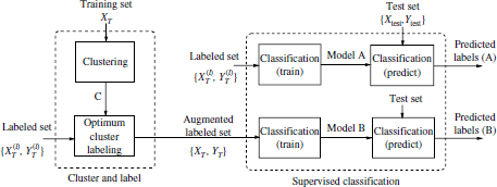
4.2.1. Block diagram
The block diagram of the semi-supervised approach is illustrated in Figure 4.1. It consists of two main parts: cluster and label and supervised classification.
Figure 4.1. Block diagram of the semi-supervised algorithm
4.2.1.1. Dataset
First, the data are divided into a test set (~ 10%) and a training set (~ 90%). Let
![]()
denote the training data, where l refers to the labeled seed size and u the size of the unlabeled seed. The total training size considering both labeled and unlabeled portions is thus l + u. This training set can be divided into two disjoint subsets:
![]()
where ![]() denotes the subset of unlabeled patterns in
denotes the subset of unlabeled patterns in ![]() T and
T and ![]() the labeled portion of
the labeled portion of ![]() T for which the corresponding set of labels
T for which the corresponding set of labels ![]() is (assumed to be) known. Hence, the initial labeled set can be expressed as the set of pairs:
is (assumed to be) known. Hence, the initial labeled set can be expressed as the set of pairs:
![]()
with the set of (manual) labels, ![]() . The block diagram of the algorithm is shown in Figure 4.1. The two main parts in the semi-supervised strategy are the cluster and label block, and the supervised classification in which a supervised model is trained with the augmented dataset from the cluster and label block. The test set is denoted as the pairs {
. The block diagram of the algorithm is shown in Figure 4.1. The two main parts in the semi-supervised strategy are the cluster and label block, and the supervised classification in which a supervised model is trained with the augmented dataset from the cluster and label block. The test set is denoted as the pairs {![]() test,
test, ![]() test} of test instances and labels. A fully supervised version is also depicted in the upper branch of the supervised classification block. In this case, the supervised classifier is trained with the initial labeled seed:
test} of test instances and labels. A fully supervised version is also depicted in the upper branch of the supervised classification block. In this case, the supervised classifier is trained with the initial labeled seed: ![]() .
.
4.2.1.2. Clustering
The first step in the semi-supervised approach is to find a cluster partition ![]() of the training data XT into a set of k disjoint clusters
of the training data XT into a set of k disjoint clusters ![]() = {C1, C2,…,Ck}, where k is the number of classes. In this work, the partitioning around medoids (PAM) algorithm has been applied. As explained in Chapter 2, the PAM algorithm provides the optimum cluster partition with the minimum sum of distances to the cluster medoids. The clustering task can be expressed as an implicit mapping function, FC, that assigns each training instance into one of the clusters in
= {C1, C2,…,Ck}, where k is the number of classes. In this work, the partitioning around medoids (PAM) algorithm has been applied. As explained in Chapter 2, the PAM algorithm provides the optimum cluster partition with the minimum sum of distances to the cluster medoids. The clustering task can be expressed as an implicit mapping function, FC, that assigns each training instance into one of the clusters in ![]() :
:
4.2.1.3. Optimum cluster labeling
The labeling block performs a crucial task in the semi-supervised algorithm. Given the set of clusters ![]() in which the training data are divided, the objective of this block is to find an optimum objective mapping of labels to clusters,
in which the training data are divided, the objective of this block is to find an optimum objective mapping of labels to clusters,
![]()
so that an optimum criterion is fulfilled. Each cluster has been assigned exactly one class label in ![]() . Assuming a fixed ordering of the clusters extracted by the PAM algorithm, {C1, C2,…,Ck}, the objective of the cluster labeling block is to find a permutation of the class labels corresponding to the ordered set of clusters. By labeling each cluster with one of the class labels in
. Assuming a fixed ordering of the clusters extracted by the PAM algorithm, {C1, C2,…,Ck}, the objective of the cluster labeling block is to find a permutation of the class labels corresponding to the ordered set of clusters. By labeling each cluster with one of the class labels in ![]() , all data instances in the training set
, all data instances in the training set ![]() T remain implicitly labeled with the class label of their respective clusters. In mathematical terms, the optimum cluster labeling provides an estimation
T remain implicitly labeled with the class label of their respective clusters. In mathematical terms, the optimum cluster labeling provides an estimation ![]() i of the optimum class label for each observation xi in the training set:
i of the optimum class label for each observation xi in the training set:
![]()
As a result of cluster labeling, the initial labeled seed ![]() is extended to the complete training data. This augmented labeled set can be expressed as
is extended to the complete training data. This augmented labeled set can be expressed as
![]()
where ![]() T denotes the set of augmented labels corresponding to the observations in
T denotes the set of augmented labels corresponding to the observations in ![]() T. For training instances in the labeled seed, the available manual labels are selected. For unlabeled patterns,
T. For training instances in the labeled seed, the available manual labels are selected. For unlabeled patterns, ![]() , the augmented label is the class label estimation
, the augmented label is the class label estimation ![]() i obtained by the optimum cluster labeling.
i obtained by the optimum cluster labeling.
The optimum cluster labeling block is explained in more detail in section 4.3.
4.2.1.4. Classification
Finally, a supervised classifier is trained with the augmented labeled set (![]() T,
T, ![]() T) obtained after cluster labeling. The learned model is then applied to predict the labels for the test set.
T) obtained after cluster labeling. The learned model is then applied to predict the labels for the test set.
Simultaneously, a fully supervised classification scheme has been compared with the semi-supervised algorithm. In this case, the classifier is directly trained with the initial labeled seed (![]() (l),
(l), ![]() (l)). The (supervised) model (denoted as model A in Figure 4.1) is again applied to predict the labels of the test data.
(l)). The (supervised) model (denoted as model A in Figure 4.1) is again applied to predict the labels of the test data.
Both semi-supervised and supervised strategies have been evaluated in terms of accuracy, by comparing the predicted labels of the test patterns with their respective manual labels. The evaluation results are discussed in section 4.6.
4.3. Optimum cluster labeling
This section describes the objective criterion applied to the optimum cluster labeling and the algorithms used to achieve this optimum.
4.3.1. Problem definition
Given the training data, ![]() of labels associated with th e portion
of labels associated with th e portion ![]() of the training set, the set
of the training set, the set ![]() of labels for the k existing classes,1 and a cluster partition
of labels for the k existing classes,1 and a cluster partition ![]() of
of ![]() T into disjoint clusters, the optimum cluster labeling problem is to find an objective mapping function, L:
T into disjoint clusters, the optimum cluster labeling problem is to find an objective mapping function, L:
![]()
which assigns each cluster in ![]() to a class label in
to a class label in ![]() , while minimizing the total labeling cost. This cost is defined in terms of the labeled seed
, while minimizing the total labeling cost. This cost is defined in terms of the labeled seed ![]() and the set of clusters
and the set of clusters ![]() . Consider the following matrix of overlapping products O:
. Consider the following matrix of overlapping products O:
[4.1] 
with constituents nij, denoting the number of labeled patterns from ![]() with class label y = i that fall into cluster Cj. The labeling objective is to minimize the global cost of the cluster labeling denoted by L:
with class label y = i that fall into cluster Cj. The labeling objective is to minimize the global cost of the cluster labeling denoted by L:
[4.2] ![]()
where W = (w1,…,wk) is a vector of weights for the different clusters. These weights may be used if significant differences in the cluster sizes are observed. In this book, the weights are assumed to be equal for all clusters, so that wi = 1, ∀i ∈ 1…k.
The individual of labeling a cluster Ci with class j is defined as the number of samples from class j (in the labeled seed) which fall outside the cluster Ci, i.e.,
[4.3] ![]()
by applying equation [4.3] into the total cost definition of equation [4.2], yields
[4.4] ![]()
Using a greedy search algorithm, the cost minimization of equation [4.2] requires k! operations (where k denotes the number of clusters/classes). Such a complexity becomes computationally intractable for k ≥ 10. However, larger number of classes are often involved in real classification problems. In this book, two popular optimization algorithms have been applied to achieve the optimum cluster labeling with substantially lower complexities:
– The Hungarian algorithm by Huhn and Monkres and
– the genetic algorithms (GAs).
Both algorithms require the definition of a cost matrix C[kxk], whose rows denote the clusters and the columns are referred to class labels in ![]() . The elements Cij denote the individual costs of assigning the cluster Ci to class label j, i.e. Cij = cost(L(Ci) = j).
. The elements Cij denote the individual costs of assigning the cluster Ci to class label j, i.e. Cij = cost(L(Ci) = j).
More details about the Hungarian algorithm and GA applied to solve the optimum cluster labeling problem are described in sections 4.3.2 and 4.3.3.
4.3.2. The Hungarian algorithm
The Hungarian method is a linear programing approach which solves the assignment problem in ![]() (N)3 operations [KUH 55,GOL 03]. The algorithm was devised by Huhn in 1955. Its name, “Hungarian,” was given after two Hungarian scientists who had previously established a large part of the algorithm’s mathematical background.
(N)3 operations [KUH 55,GOL 03]. The algorithm was devised by Huhn in 1955. Its name, “Hungarian,” was given after two Hungarian scientists who had previously established a large part of the algorithm’s mathematical background.
Although the algorithm’s complexity was originally ![]() (N4), a more recent version with complexity
(N4), a more recent version with complexity ![]() (N3) was developed by Huhn and Monkres, thus referred to as the Huhn-Monkres algorithm.
(N3) was developed by Huhn and Monkres, thus referred to as the Huhn-Monkres algorithm.
The algorithm states the assignment problem in terms of bipartite graphs. In the following paragraphs, some important notions from graph theory are introduced.
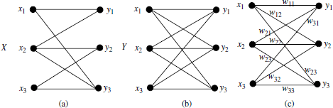
4.3.2.1. Weighted complete bipartite graph
DEFINITION 4.1.– Bipartite graph: a bipartite graph is a graph, G(![]() ,
, ![]() ), with set of vertices
), with set of vertices ![]() and set of edges
and set of edges ![]() , in which two disjoint subsets of
, in which two disjoint subsets of ![]() can be found,
can be found, ![]() and
and ![]() , with no internal edges connecting two vertices within a subset. Thus, the set of edges
, with no internal edges connecting two vertices within a subset. Thus, the set of edges ![]() only connects any vertex in
only connects any vertex in ![]() with any of the vertices of
with any of the vertices of ![]() . In the following, a bipartite graph is also denoted G(
. In the following, a bipartite graph is also denoted G(![]() ,
,![]() ,
,![]() ).
).
DEFINITION 4.2.– (Complete weighted bipartite graph): a complete bipartite graph is a bipartite graph in which, for all pairs (x, y) of vertices from ![]() and
and ![]() , there exists an edge,
, there exists an edge, ![]() , that connects x with y.
, that connects x with y.
DEFINITION 4.3.– (weighted complete bipartite graph): a weighted complete bipartite graph is a complete bipartite graph in which each edge, ex,y, is assigned to a certain weight w(x,y). Note that a value of w(x,y) = 0 is also possible, and the weighted bipartite graph is still complete.
Figure 4.2 shows three examples of the bipartite graph, the complete bipartite graph, and the weighted complete bipartite graph, respectively.
Figure 4.2. Example of bipartite graphs: (a) bipartite graph with two disjoint subsets, (b) complete bipartite graph, and (c) completed weighted bipartite graph
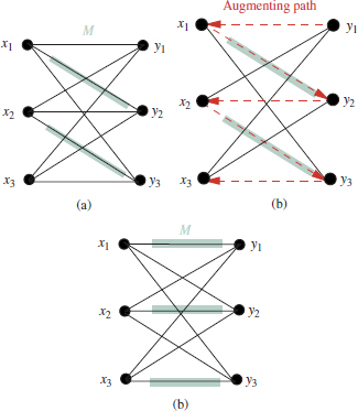
4.3.2.2. Matching, perfect matching and maximum weight matching
DEFINITION 4.4.– (Matching): a matching M, defined on a graph G(![]() ,
, ![]() ,
, ![]() ), is any subset of edges, M ∈
), is any subset of edges, M ∈ ![]() , such that no common vertex is shared between different edges in M (Figure 4.3(a)).
, such that no common vertex is shared between different edges in M (Figure 4.3(a)).
DEFINITION 4.5.– (Perfect matching): a perfect matching is a matching M in which each vertex x is connected to a vertex y by an edge in M (Figure 4.3(b)).
DEFINITION 4.6.– (Maximum weight matching): denoting ![]() , the set of all possible perfect matchings in G(X;Y;E), the maximum weight matching is the perfect matching M′ ∈
, the set of all possible perfect matchings in G(X;Y;E), the maximum weight matching is the perfect matching M′ ∈ ![]() . in which the sum of edge weights is maximum:
. in which the sum of edge weights is maximum:
Figure 4.3. Example of matching in bipartite graphs. (a) Arbitrary matching, M and (b)Complete bipartite graph

4.3.2.3. Objective of Hungarian method
Given the above introductory definitions regarding bipartite graphs, the objective of the Hungarian algorithm is to find the maximum weight matching M′ in a complete bipartite graph, G(X, Y, E).
Two fundamental notions that allow us to significantly reduce the search space of perfect matchings ![]() to find the maximum weight matching are the concepts of vertex labeling and equality graphs.
to find the maximum weight matching are the concepts of vertex labeling and equality graphs.
DEFINITION 4.7.– (Feasible vertex labeling): a feasible vertex labeling upon a weighted bipartite graph G(X, Y, E) is a function that assigns a label, ![]() to each vertex in V, such that the sum of labels of any pair of vertices connected by an edge ex,y is greater than equal to the edge weight wxy,
to each vertex in V, such that the sum of labels of any pair of vertices connected by an edge ex,y is greater than equal to the edge weight wxy,
![]()
DEFINITION 4.8.– (Equality (subgraph):) given a feasible vertex labeling, l, the equality subgraph of a complete bipartite graph is the graph Gl(X,Y,El) defined by the vertices in X and Y and a subset of edges El ∈ E, whose weights wxy are strictly equal to the sum of vertex labels l(x) + l(y):
![]()
Given the vertex labeling and equality subgraph definitions, the basis of the Hungarian algorithm is the Huhn — Monkres theorem.
Theorem 4.1. (Huhn — Monkres theorem): if a perfect matching is found in an equality subgraph of G(X, Y, E), this matching is the maximum weight matching.
Proof 1. From the definition of feasible labeling, any edge (x, y) ∈ E satisfies that
For a perfect matching M, each vertex is only adjacent to one edge, thus,
[4.7] ![]()
Now, any edge ex,y in an equality graph satisfies
Hence, for any perfect matching over the equality graph, Ml, it yields
Finally, by merging equations [4.7] and [4.10]
[4.10] ![]()
Thus, the problem of finding a maximum weighted matching is transformed into the one finding a feasible vertex labeling with a perfect matching in the associated equality subgraph. This is essentially achieved by selecting an initial vertex labeling as well as a matching M, of size |M|, in the equality graph, and iteratively growing M until it becomes a perfect matching (|M| = k). In each iteration, the size of M is increased by one edge after an augmented path is found.
DEFINITION 4.9.– (Path): a path over a graph G(V,E)is defined as a sequence of vertices {v1, v2, v3, v4,…,vp}, such that there exists an edge connecting each pair of vertices (vi,vi+l). Note that the superscripts 1,2,…,p are not referred to the indices of the vertices in the graph, but to their order in the path sequence.
DEFINITION 4.10.– (Augmented path): given a matching M in the equality graph, an augmented path is a path (1) whose edges alternate between M and ![]() (alternating path), and (2) whose start and end vertices, v1 and vp, are unmatched, i.e.,
(alternating path), and (2) whose start and end vertices, v1 and vp, are unmatched, i.e., ![]() .
.
Obviously, if an augmented path is found, the size of M can be increased by one edge by inverting the edges in the path from ![]() → M and M →
→ M and M → ![]() so that the new path can be expressed as (Figure 4.4(a)) {(v1,v2) ∈ M, (v2,v3) ∈
so that the new path can be expressed as (Figure 4.4(a)) {(v1,v2) ∈ M, (v2,v3) ∈ ![]() ,…,(vi, vi+1) ∈ M} (Figure 4.4(b)).
,…,(vi, vi+1) ∈ M} (Figure 4.4(b)).
As mentioned earlier, the Hungarian algorithm starts by an arbitrary vertex labeling. Typically, the labels for the vertices in Y are set to 0, while each vertex xi ∈ X is labeled with the maximum of its incident edges,
Figure 4.4. Illustration of augmented paths. (a) Bipartite graph with two disjoint subsets and an arbitrary matching M; (b) Alternating path with start at y1 and end at x3. The vertex order is indicated by the arrows. (c) The alternating path allows us to increase the matching M, resulting in a perfect matching
Then, a matching in the equality graph, El, associated with the vertex labeling is selected. If |M| = k, this matching is already perfect and the optimum is found. If the matching is not perfect, the size of M needs to be gradually incremented in a number of iterations. By definition 4.10, |M| can be increased by one edge if an augmenting path is found. Thus, each iteration step is directed toward the search for an augmented path.
As M is not yet perfect, there must be some unmatched vertex x ∈ ![]() connected to a matched vertex y. This seems to be obvious, since otherwise the vertex xi would be already matched in M. Let Nl(x) denote the subset of vertices in
connected to a matched vertex y. This seems to be obvious, since otherwise the vertex xi would be already matched in M. Let Nl(x) denote the subset of vertices in ![]() which are connected to x (the neighbors of x). Also, let X′ denote the subset of vertices X′ ∈
which are connected to x (the neighbors of x). Also, let X′ denote the subset of vertices X′ ∈ ![]() − {x} matched to any vertex in Nl(x). Thus, x is “competing” with X′ for an edge in M. The path {x,y,x′ ∈ X′} can be thought of as a section of an augmented path. Now, if an unmatched vertex y′ is found, connected to any vertex in S = {X′ ∪ xi} in a (new) equality graph, two situations may occur:
− {x} matched to any vertex in Nl(x). Thus, x is “competing” with X′ for an edge in M. The path {x,y,x′ ∈ X′} can be thought of as a section of an augmented path. Now, if an unmatched vertex y′ is found, connected to any vertex in S = {X′ ∪ xi} in a (new) equality graph, two situations may occur:
1. y′ is connected to x. Then, M can be increased by adding a new edge {x,y′). The new matching can be expressed as M′ = M ∪(x,y′),
2. y′ is connected to a vertex in X′. Let this vertex be denoted as x2, and y2, the vertex in ![]() matched to x2. Then, an augmented path can be found in the form x,y2,x2,y′, and M can be incremented by inverting the path edges from M to
matched to x2. Then, an augmented path can be found in the form x,y2,x2,y′, and M can be incremented by inverting the path edges from M to ![]() and vice versa.
and vice versa.
Now, assuming that a maximum size matching M has been previously selected, the required unmatched vertex y′ does not yet exist in El. Otherwise, this vertex would already be included in M. Therefore, the equality graph El must be expanded to find new potential vertices in Y to augment M. Obviously, the expansion of El requires a vertex (re)labeling l′. It is formulated as

The relabeling function l′ ensures that a new equality graph is found, ![]() , such that
, such that ![]() ∈ El and some new edge
∈ El and some new edge ![]() exists. In other words, the new set of S neighbors in
exists. In other words, the new set of S neighbors in ![]() .
.
Consider the new edges ![]() in
in ![]() . With reference to the vertex y, two possible cases are to be considered:
. With reference to the vertex y, two possible cases are to be considered:
– ![]() (y is not matched). Thus, an augmented path can be found and |M′| = |M| + 1.
(y is not matched). Thus, an augmented path can be found and |M′| = |M| + 1.
– ![]() (y is matched). The new edge can be expressed as
(y is matched). The new edge can be expressed as ![]() . Since y is not an unmatched vertex, the path cannot be augmented. In this case, the vertex x′ matched to y is attached to S so that y belongs to
. Since y is not an unmatched vertex, the path cannot be augmented. In this case, the vertex x′ matched to y is attached to S so that y belongs to ![]() Then, a new vertex relabeling is required, forcing new edges in
Then, a new vertex relabeling is required, forcing new edges in ![]() connecting vertices from S to Y −
connecting vertices from S to Y − ![]() . Such vertex labeling is iterated, adding vertices to S and Nl(S) until an unmatched vertex in Y is found.
. Such vertex labeling is iterated, adding vertices to S and Nl(S) until an unmatched vertex in Y is found.
Each time |M| is incremented, the previous steps are repeated, starting with another free vertex in X. This process is iterated until all free vertices in X are explored, in which case |M| = k and a perfect matching (the maximum weight matching) is achieved.
4.3.2.4. Complexity considerations
In each phase of the Hungarian method, the size of the matching |M| is incremented by one edge. Thus, the perfect matching is attained in a maximum of k phases. As explained earlier, within each phase, a vertex relabeling is required to find a free vertex ![]() . If the size of the matching at phase i is |Mi|, a maximum number of relabeling steps |Mi| − 1 is required in the worst case. Thus, each phase requires at most |M| − 1 iterations. Typically, the upper bound for such complexity is stated as O(k). Finally, each relabeling requires, in principle, a total number of k2 operations. However, with an adequate implementation this complexity can be reduced to O(k). Thus, the total complexity of the Hungarian method is O(k) phases ·O(k) relabelings ·O(k)= O(k3).
. If the size of the matching at phase i is |Mi|, a maximum number of relabeling steps |Mi| − 1 is required in the worst case. Thus, each phase requires at most |M| − 1 iterations. Typically, the upper bound for such complexity is stated as O(k). Finally, each relabeling requires, in principle, a total number of k2 operations. However, with an adequate implementation this complexity can be reduced to O(k). Thus, the total complexity of the Hungarian method is O(k) phases ·O(k) relabelings ·O(k)= O(k3).
4.3.3. Genetic algorithms
In the early 1970s, John Holland invented an algorithmic paradigm which attempted to solve engineering problems by closely observing nature. Such algorithms showed an extraordinary potential to solve a variety of complex problems, outperforming traditional approaches.
Inspired by Darwin’s discoveries — the laws of natural selection, inheritance, genetics and evolution — this kind of algorithm was named GA [DAV 91,GOL 89].
From evolution theory, natural selection is governed by the “survival of the fittest” law. According to this principle, those living structures that perform well under certain environmental conditions tend to survive, unlike those that fail to adapt to the environment.
This evolutionary principle forms the basis for GAs. The environment is modeled by the optimization criterion (objective function), while the individuals are represented by their chromosomes. Natural selection ensures that only the genetic material of the best individuals is preserved in the next generations. In terms of GAs, the former is achieved by an appropriate parent selection strategy. Also, the evolution from one generation to the next one is present in the form of reproductory operators. In each new generation, the chromosomes are generally better “adapted” to the environment (quality criterion), which implies that the GA is evolving toward an optimum of the objective function. By representing the solution space in a chromosomal form, each particular value of a chromosome encodes a possible solution to the objective function (environment). The optimum solution is thus given by the value of the fittest chromosome in a convergence status.
In general terms, a GA can be described by the following steps:
1.Initialize a random population of chromosomes.
2.Evaluate chromosomes on the basis of their fitness values.
3.Using a suitable parent selection strategy, pick a number of chromosomes into the “mating pool” of parent. chromosomes
4.Perform reproduction operators (crossover and mutation) on the mating pool members to form child chromosomes. The next generation is formed using a suitable population formation strategy.
5.If the termination criterion is fulfilled, the fittest chromosome in the current population can be regarded as the “winning” chromosome — optimum solution. Otherwise, go to step 2.
In the following sections, an brief overview of reproduction operators is presented.
4.3.3.1. Reproduction operators
Two types of reproduction can be functionally distinguished. Reproduction operators used in GA are inspired by the biological concepts of sexual/asexual reproduction. By means of sexual operators (crossover), the genetic material of two parent individuals is combined to form children chromosomes. In contrast, asexual operators (mutation) produce random changes in single genes, gene positions, or gene substrings in a chromosome. Crossover and mutation operators are explained in detail in the following paragraphs.
4.3.3.1.1. Crossover
As explained earlier, crossover operators require the participation of two parent chromosomes to form the children chromosomes. Different types of crossover operators may be applied within a GA. However, one essential factor to take into consideration for choosing crossover types is the “context sensitivity.” As certain crossover types may suit a certain chromosome representation, they may produce invalid chromosomes for other representation. If the crossover type produces invalid chromosomes, the GA must be aware of these situations and reject any possible invalid solution.
– One point crossover: in this type of crossover, a point within the chromosome’s length is randomly selected. The genetic material of the two parents beyond this point is swapped to form the children.
– k- point crossover: this operator is a generalization of the one-point crossover. k points along the chromosome length are selected, swapping the genetic material of the parents between each pair of consecutive points.
– Uniform-based crossover: while the previous operators are only suitable for binary chromosome representation, the uniform-order-based crossover was proposed by Davis [DAV 91] for the permutation representation of chromosomes. First, a binary mask of the same length as that of a chromosome is randomly selected. This mask determines which child inherits each gene and from which parent, in particular. As an example, if bit i is active (‘1’), child 1 inherits gene at position i from parent 1. If the bit is inactive (‘0’), child 2 inherits the gene from parent 2. The missing gene values — corresponding to the positions of the mask inactive bits in child 1 and active bits for child 2 — are filled in the remaining gene positions of children 1 and 2, preserving their order of appearance in parents 2 and 1, respectively.
– Partially mapped crossover: also devised for the chromosome permutation representation, this operator is similar to the uniform-order-based crossover. The gene positions to be copied from parents 1 and 2 in children 1 and 2 are specified by a random binary mask, as explained earlier for the uniform-order-based crossover. Then, the child chromosomes 1 and 2 are completed with the missing gene values, preserving the order and position as they appear in parents 2 and 1, respectively, to the highest possible extent.
4.3.3.1.2. Mutation
A variety of mutation types have been proposed in the GA literature for asexual reproduction. In the following, five popular mutation operators are described.
– Simple bit mutation: This operator, defined for binary chromosome representation is the simplest mutation operators. An intrinsic parameter of the bit mutation strategy is the bit mutation rate, m ∈ [0,1]. It indicates a maximum threshold for mutant genes. Mutant genes is identified as follows: First, each gene in a chromosome is assigned a random value, p ∈ [0,1] from a uniform probability distribution. Mutant genes are those with p ≤ m. If a gene is identified as mutant, it means that its value can be reversed (0 → 1,1 → 0) with probability 0.5.
– Flip bit mutation: this operator is very similar to the simple bit mutation, but differs in that the value of a mutant gene is always reversed (with probability 1.0). Thus, the effective mutation rate is doubled with respect to the simple bit mutation.
– Swapping mutation: this operator performs a simple mutation, which is applicable to many types of the chromosome representation. It simply selects two random positions along a chromosome, and exchanges the genes at these positions.
– Sliding mutation: as with swapping mutation, this operator can be used with many different types of chromosome representation. Again, two points within a chromosome’s length are selected, i, j, with i < j − 1. The segment of genes at indexes i + 1 to j slided by one position to the left, pushing the gene at position i to position j. In vectorial form, the sliding mutation operator can be expressed as follows:
– Scramble bit mutation: this operator was proposed by Davis [DAV 91] for the permutation representation of chromosomes. It selects a substring of genes and combines them randomly, leaving the rest of the genes unchanged.
4.3.3.2. Forming the next generation
An overview is now provided of the strategies to form the next generation from the current population of chromosomes. In particular, three approaches are described: generational replacement, elitism and generational replacement, and steady-state representation.
4.3.3.2.1. Generational replacement
Using this strategy, the parent generation is entirely replaced by a new population of children chromosomes obtained by crossover and mutation. One limitation of generational replacement is associated with these reproductory operators. As previously explained, according to the survival of the fittest principle, fittest individuals are selected into the mating pool of parent chromosomes. Crossover and mutation operators may, nevertheless, destroy good schemata present in parent chromosomes, by combining or mutating the genes within a schema.
4.3.3.2.2. Elitism with generational replacement
This method attempts to overcome the aforementioned limitation of simple generational replacement through the introduction of elitism or “elite selection.” In the frame scope of GAs, the term “elite” refers to the top fittest chromosomes in a population. Denoting P, the population size and e, the elite selection rate, the top |e · P| fittest chromosomes are identified as elite chromosomes or super-individuals. An exact copy of each elite chromosome is then passed to the next generation. The remaining P − eP children are then produced by simple generational replacement. According to Davis, a small value of the elite selection rate e may be beneficial for the GA performance, since it ensures that fit chromosomes with good schemata are preserved in the next generations. In contrast, large values of this parameter can lead to degradations in the GA performance, or slow down the convergence, due to the subsequent reduction in the “active” search space (in terms of population chromosomes).
4.3.3.2.3. Steady state representation
This method replaces only the m chromosomes with the poorest fitness values in a population, keeping exact copies of the P − m remaining chromosomes. Obviously, the steady-state reproduction is equivalent to elitism for m = P and corresponds to elitism with generational replacement with an elite parameter e = P − m.
4.3.3.3. GAs applied to optimum cluster labeling
In this book, GAs have been applied to solve the cluster labeling problem. As explained in Section 4.3, the cluster labeling objective is equivalent to find an optimum permutation of class labels, by considering a fixed ordering of the clusters (C1toCk). For this reason, a permutation representation style has been used as chromosome encoding:
![]()
In the chromosome, cluster labels are encoded by the gene positions, whereas class labels are indicated by the gene values, i.e. πk = L(Ck). For example, if the gene at position i has a value πi = j, the ith cluster is assigned to class label L(Ci)= j.
The evaluation of a chromosome is defined as the total cost definition (equation [4.4]) of wrong cluster—class label assignments associated with the class label permutation. In terms of the chromosome gene values, the labeling cost can be expressed as
[4.16] 
Thus, the fitness function that allows us to identify the top chromosomes in a population can be defined as the inverse of equation [4.16]:
Note that the inverse of the labeling cost, or fitness, corresponds in this case to the total overlap of class labels due to the following conditions:
– The weight factors in the labeling cost formulation in equation [4.2] are not taken into account (all weights are set to 1).
– The number of labeled examples in the labeled seed is considered constant for all categories.
Owing to the first condition, the cost formula can be expressed as
[4.18] 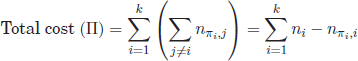
where ni denotes the number of labeled examples in the initial seed for the class label indicated by the gene πi. As this value is constant for all class labels, i.e., n1 = n2 = …, = nk = n, the cost in equation [4.18] can be also formulated as
[4.19] 
Hence, the chromosome fitness can be identified as the sum of overlapping products in the second term of equation [4.19].
As for parent selection, a simple tournament selection strategy has been selected. This approach divides the population in equally sized blocks, each with M chromosomes. Then, it selects the N fittest chromosomes from each block into the mating pool. In this book, different values of M have been applied, namely, M = 5, M = 10, and M = 11. In all cases, two fittest parents are selected from each block (N = 2).
Generational replacement with elitism is the method selected to form the next generation, using different types of crossover and mutation to obtain the genetic material of the children from their parent’s chromosomes. Now, the new generation is formed in blocks of M chromosomes. For the first block, the first two parents in the mating pool are selected. The block is filled with M children, obtained from crossovers and mutations from their corresponding two parents. The same is applied for the rest of blocks, using the second, third, etc., pairs of parents in the mating pool. Let cr and (mr) denote the crossover and effective mutation rates applied to the GAs, respectively. Different crossover and effective mutation rates have been compared, depending on the block size M. For M = 5, two children are generated with crossover (cr = 2/5) and three children with mutations (mr = 3/5). For M = 10, the crossover and mutation rates have been set to cr = 6/10 and mr = 4/10. Likewise, for M = 11, cr = 10/11 and mr = 1/11.
4.3.3.4. Comparison of methods
In the following, the performances of the Hungarian algorithm and GAs for the optimum assignment problem are compared by means of a controlled experiment. As both strategies have been devised for the cluster labeling problem, artificial confusion matrices have been synthesized. They are possible real situations with clusters/class labels. A confusion matrix represents the number of class labels (rows) that fall into the different clusters (columns), with the particularity that the elements in the diagonal correspond to the best cluster-class matchings. The matrix overlapping products O in equation [4.1] can be transformed into a confusion matrix, O′, by re-arranging the row elements according to the optimum class label permutation. In this case, the sum of values in the diagonal of O′ gives the maximum overlap (minimum of equation [4.2]).
Ideally, the cluster partition of a dataset should perfectly match the underlying class distribution. The resulting confusion matrix is thus a diagonal matrix. However, in most real problems, clusters may deviate from the true classes to a certain extent. This may be due to the inadequate choice of a cluster algorithm that does not fit into the true data distribution, the existence of ambiguities in the dataset, or even the presence of errors in the manual labels. To analyze the cluster labeling performance of the Hungarian algorithm and GAs under these circumstances, the artificial matrices used in this work are intended to reproduce and quantify their potential effects on the confusion matrix O′.
First, it is assumed that each class can be optimally represented by one of the clusters. It is, namely, the cluster that provides the best coverage of the elements in the class. In a non-ideal situation, a certain amount of labeled patterns may fall outside their “representative” cluster, as a sort of interference to the receiver clusters. Two variables have been used to model these situations:
– Variable ratio of “escaping” labels (E): given a number of labels per category, n, and summing each class to be optimally represented by a certain cluster C(opt), this variable indicates the ratio of class labels that “escape” outside cluster C(opt) to other neighbor clusters (also referred to as receiving clusters). For example, if L = 20 and E = 0.5, 10 labels of the given class escape cluster C(opt). This variable ratio of escaping patterns is a uniformly distributed variable in the range E ∈ [0−Emax], where Emax < 1 is a parameter of choice. In this book, different values of Emax have been applied to “control” the complexity of the cluster labeling problem.
– Variable number of receiving clusters Rx: this variable indicates a number of (undesired) clusters that are recipient of the escaping patterns. Again, this is a uniform random variable in the range Rx ∈ [0, Rxmax], where Rxmax < k is a parameter specified by the user. Note that the escaping patterns are not homogeneously distributed through the recipient clusters. Instead, it is assumed that some clusters are somewhat closer to the desired cluster C(opt) than others and should therefore receive a larger number of labels than more distant clusters. Hence, a number of labels that fall into the clusters is generated according to a triangular filter centered in the diagonal element, whose weights add to 1. Rx values are obtained, which are randomly rearranged to occupy the row positions adjacent to the diagonal elements.
Four of the artificial confusion matrices used in the experiments are shown in Figure 4.5, which represent potential clusterings with k = 20 clusters/classes. These matrices are referred to four different combinations of values for (Emax, Rxmax): (0.2,12), (0.2,5), (0.9,12), and (0.9,5) (Figure 4.5(a–d), respectively).
Figure 4.6 shows the labeling performance of the Hungarian algorithm and the three implementations of GAs, with effective mutation rates of mr = 3/5, 4/10, and 1/11. In the plots, these three implementations of the GA are referred to as GA1, GA2, and GA3, respectively. The labeling performance is depicted in terms of GA generations required to achieve the optimum labeling (minimum labeling error). Thus, the performance of the Hungarian algorithm is plotted as a constant value.
Figure 4.5. Artificial confusion matrices used to represent the . cluster labeling problem, with different values of the parameters, E and Rx. (a) E = 0.2, Rx = 15; (b) E = 0.2, Rx = 5; (c) E = 0.9, Rx = 15; (d) E = 0.9,Rx = 5
As can be observed, the most effective GA implementation is the one with the highest effective mutation rate (GA3). It achieves the optimum in around 40 generations, with minimum variations regardless of the different confusion matrices. As the mutation rate decreases, the GA convergence slows down significantly. As an example, The GA1 implementation (mr = 3/5) requires a double number of generations for convergence with respect to the other two implementations for Emax = 0.2 and almost a triple number of iterations for Emax = 0.9.
Figure 4.6. Cluster labeling error produced by the GA and Hungarian algorithm on the confusion matrices in Figure 4.5. (a) E = 0.2, Rx = 15; (b) E = 0.2, Rx = 5; (c) E = 0.9, Rx = 15; (d) E = 0.9,Rx = 5

Given the previous explanations, the GA3 implementation of the GA has been the one selected in this work to solve the cluster labeling problem in real clustering tasks.
4.4. Supervised classification block
The final stage of the semi-supervised approach developed in this book is the supervised classification block. The basic difference of the semi-supervised strategy versus a fully supervised approach relies on the labeled set which is fed to this block. In the semi-supervised approach, the supervised classification is fed with the augmented labeled seed from the cluster labeling step. The supervised counterpart is attained when the initial labeled seeds are directly used to train this classification block instead. According to the block diagram in Figure 4.1, the supervised classification block is defined in generic terms. In practice, any supervised classifier available in the ML literature can be applied by just adapting the necessary software interface (a function call in R). In this work, two popular classification models have been applied to the supervised classification block: support vector machines (SVMs) and, for a dataset of utterances (see section 4.5.3), the naive Bayes rule. These algorithms are described in more depth in the following paragraphs.
4.4.1. Support vector machines
SVMs are among the most popular classification and regression algorithms because of their robustness and good performance in comparison with other classifiers [BUR 98, JOA 97, LIN 06]. In its basic form, SVM were defined for binary classification of linearly separable data. Let ![]() denote a set of training patterns
denote a set of training patterns ![]() = {x1,x2,…xL} in
= {x1,x2,…xL} in ![]() D. For binary classes, the possible class labels corresponding to the training data elements (
D. For binary classes, the possible class labels corresponding to the training data elements (![]() = {y1,…,yL}) are yi ∈ {1,−1} (Figure 4.7).
= {y1,…,yL}) are yi ∈ {1,−1} (Figure 4.7).
Assuming that the classes (+1,−1) are linearly separable, the SVM goal is to orientate a hyperplane H that maximizes the margin between the closest members of the two classes (also called support vectors). The searched hyperplane is given by equation [4.20],
Figure 4.7. SVM example of binary classification through hyperplane separation (in this two-dimensional case the hyperplane becomes a line)

[4.20] ![]()
denoting w the normal vector of the hyperplane. In addition, the parallel hyperplanes H1 and H2 at the support vectors of classes y = 1 and y = −1 are defined as
It can be demonstrated that the margin between the hyperplanes H1 and H2 is ![]() . In addition, the training points at the left/right sides of the hyperplanes H1 and H2 need to satisfy
. In addition, the training points at the left/right sides of the hyperplanes H1 and H2 need to satisfy
Thus, the maximum margin hyperplane is obtained by solving the following objective:
[4.23] ![]()
By applying Lagrange multipliers, the objective in equation [4.23] can be solved using constrained quadratic optimization. After some manipulations, it can be shown that the initial objective is equivalent to
The solution of this quadratic optimization problem is a set of coefficients α = {α1,…,αL}, which are finally applied to calculate the hyperplane variables ω and b:
[4.25] 
where ![]() denotes the set of support vectors of size Ns.
denotes the set of support vectors of size Ns.
Although the solution in equation [4.25] is found for the basic problem of binary, linearly separable classes, SVMs have been extended for both multi-class and nonlinear problems.
4.4.1.1. The kernel trick for nonlinearly separable classes
The application of SVMs to nonlinearly separable classes is achieved by substituting the dot product xixj in equation [4.23] by an appropriate function, the so-called kernel k(xi,xj). The purpose of this “kernel trick” is that a nonlinear kernel can be used to transform the feature space into a new space of higher dimension. In this high-dimensional space it is possible to find a hyperplane to separate classes that may not be originally separable in the initial space. In other words, the kernel function is equivalent to the dot product:
where ø denotes a mapping of a pattern into the higher dimensional space. The main advantage is that the kernel computes these dot products without the need to specify the mapping function ø
4.4.1.2. Multi-class classification
The extension for the multi-class problem is achieved through a combination of multiple SVM classifiers. Two different schemes have been proposed to solve this problem: in a one-against-all approach, k hyperplanes are obtained to separate each class from the rest of classes. In a one-against-one approach, ![]() binary classifiers are trained to find all possible hyperplanes to separate each pair of classes.
binary classifiers are trained to find all possible hyperplanes to separate each pair of classes.
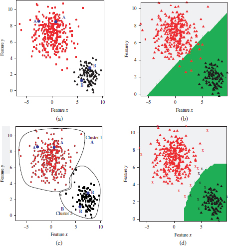
4.4.2. Example
An example of the models learned by the supervised and semi-supervised approaches in a mixture of two Gaussians is provided in Figure 4.8. In this example, two random examples per category (labeled as “A” and “B”) comprise the initial labeled seed (Figure 4.8(a)). In a supervised approach, this seed is used to train SVM model with a radial kernel. The learned hyperplane or the decision curve is depicted in Figure 4.8(b). The areas at both sides of the hyperplane are the decision regions for Gaussians A (in gray color) and B (green color). Figure 4.8(c) indicates the cluster partition of the complete data, and the corresponding cluster labeling performed by the semi-supervised approach. The so-called labeled Gaussians are used to train an SVM model. As can be observed in Figure 4.8(d), following the semi-supervised approach a more accurate hyperplane is learned, which achieves a lower number of errors on the training set in comparison to the supervised model.
Figure 4.8. Example of SVM model learned on a mixture of two Gaussians by the supervised and semi-supervised algorithms. (a) Dataset with an initial seed, whose objects are indicated by the labels “A” and “B”. (b) Model learned by SVM on the initial labeled seed. (c) Clusters and augmented labels obtained by the semi-supervised algorithm. (d) Model learned by the SVM on the augmented labeled set
4.5. Datasets
This section describes the datasets used in the experiments. As the algorithms presented in the previous sections have a general character and can be applied to any kind of features, they have been tested on several datasets from the UCI ML repository and on a corpus of utterances.
4.5.1. Mixtures of Gaussians
This dataset comprises two mixtures of five and seven Gaussians in two dimensions, where a certain amount of overlapping patterns can be observed.
4.5.2. Datasets from the UCI repository
4.5.2.1. Iris dataset (Iris)
The Iris set is one of the most popular datasets from the UCI repository. It comprises 150 instances iris of 3 different classes of Iris flowers (Iris setosa, I. versicolor, and I. virginica). Two of these classes are linearly separable while the third one is not linearly separable from the second one (Figure 4.9).
Figure 4.9. Iris dataset (projection on the three principal components)

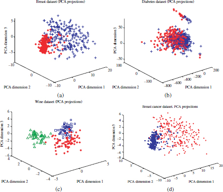
4.5.2.2. Wine dataset (wine)
The wine set consists of 178 instances with 13 attributes, representing 3 different types of wines.
4.5.2.3. Wisconsin breast cancer dataset (breast)
This dataset contains 569 instances in 10 dimensions, denoting 10 different features extracted from digitized images of breast masses. The two existing classes are referred to the possible breast cancer diagnosis (malignant and benign).
4.5.2.4. Handwritten digits dataset (Pendig)
The third real dataset is for pen-based recognition of handwritten digits. In this work, the test partition has been used, composed of 3498 samples with 16 attributes. Ten classes can be distinguished for the digits 0–9.
4.5.2.5. Pima Indians diabetes (diabetes)
This dataset comprises 768 instances with 8 numeric attributes. Two classes denote the possible diagnostics (the patients show or do not show signs of diabetes).
4.5.3. Utterance dataset
The utterance dataset is a collection of transcribed utterances collected from user calls to commercial troubleshooting agents. The application domain of this corpus is video troubleshooting. Reference topic categories or symptoms are also available.
This utterance corpus has been pre-processed using morphological analysis and stop-word removal. First, a morphological analyzer [MIN 01] has been applied to reduce the surface form of utterance words into their word lemmas. Then, the lemmatized words have been filtered using the SMART stop-word list with small modifications. In particular, confirmation words (yes, no) have been deleted from the stop word list, while some terms typical for spontaneous speech (eh, ehm, uh, …) have been included as stop words. Finally, we have retained the lemmas with two or more occurrences in the pre-processed corpus, resulting in a vocabulary dimension of 554 word lemmas. Afterwards, the pre-processed utterances have been represented in vectors of index terms using Boolean indexing — each binary component in an utterance vector indicates the presence or absence of the corresponding index term in the utterance. The final dataset is composed of 2,940 unique utterance vectors.
Figure 4.10. Projection of the datasets on the three principal components. (a) Breast dataset; (b) diabetes dataset; (c) wine; (d) Pendig
An independent test set comprising a total number of 10,000 transcribed utterances has also been pre-processed as described earlier, resulting in 2,940 unique utterance vectors. From this set, a number of utterances (~ 20% of the training set size) have been randomly selected as the test applied to the classifiers. To avoid possible biases of a single test set, 20 different test partitions have been generated. From the the training set, 20 different random seeds of labeled prototypes (n labels/category) have also been randomly selected.
4.6. An analysis of the bounds for the cluster and label approaches
As mentioned in section 4.1, the main assumption for the current cluster and label approaches is that the input data should “naturally fall into clusters.” If the data are not intrinsically organized in clusters — or the chosen clustering algorithm does not fit into the input data distribution — a cluster and label approach may yield a considerable degradation in the classification performance.
For this reason, the controlled experiment described in this section was intended to analyze the performance of the cluster and label approaches with respect to the quality of the cluster solution.
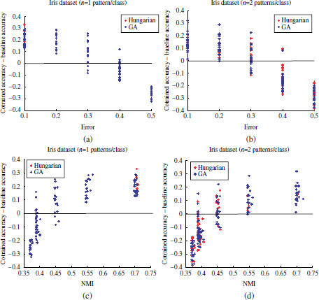
In these experiments, the Iris dataset from the UCI ML repository has been used. First, a perfect clustering has been considered equal to the set of real labels. Then, different levels of noise have been manually induced to this perfect clustering. This has been done by randomly selecting a ratio p of data patterns from each category and modifying their cluster membership from their actual cluster label yi = j to a different cluster label ![]() − j. Thus, p is also referred to as the percentage of misclassification errors. Different values of p have been applied, p = [0.1,0.2,… ,0.5]. For each p value, 20 different simulated clusterings with a ratio p of induced random noise have been generated. The equivalent normalized mutual information (NMI) between these clusterings and the real labels has also been computed. Also, for each cluster partition, 20 different labeled seeds have been randomly selected. These have been used to train both a supervised classifier and the semi-supervised algorithm with the corresponding simulated clusterings. The study has been carried out for n = 1 and n = 2 labeled samples per category.
− j. Thus, p is also referred to as the percentage of misclassification errors. Different values of p have been applied, p = [0.1,0.2,… ,0.5]. For each p value, 20 different simulated clusterings with a ratio p of induced random noise have been generated. The equivalent normalized mutual information (NMI) between these clusterings and the real labels has also been computed. Also, for each cluster partition, 20 different labeled seeds have been randomly selected. These have been used to train both a supervised classifier and the semi-supervised algorithm with the corresponding simulated clusterings. The study has been carried out for n = 1 and n = 2 labeled samples per category.
The relationship between the percentage of error and the classification performance is depicted in the scatterplots of Figure 4.11(a) and 4.11(b). Likewise, the relationships in terms of NMI values are shown in Figure 4.11(c) and 4.11(d). In both the cases, horizontal axes denote the cluster qualities (misclassification error or NMI values). Vertical axes indicate the difference in accuracy when using the semi-supervised approach with respect to the supervised SVMs (accuracy semi-supervised — accuracy supervised). Thus, any positive value in the vertical axis indicates an improvement in classification performance through the semi-supervised algorithm. Equivalently, negative values imply a degradation of the semi-supervised approach with respect to the supervised approach.
As can be observed, the accuracy of the semi-supervised classifier with respect to the supervised algorithm increases notably by decreasing the noise ratio induced to the clusterings. If the quality of the cluster partition is not sufficient to capture the underlying class structure — NMI ≤ 0.5 — the supervised approach may outperform the semi-supervised cluster and label algorithm even for n = 1. For larger NMI values, the semi-supervised algorithm achieves increasing accuracy gains with respect to the supervised approach, in consistency with the cluster assumption.
Figure 4.11. Difference in accuracy scores achieved by the semi-supervised and supervised algorithms with respect to the induced noise p and equivalent NMI parameters. (a) Accuracies of the Iris dataset, n = 1 labeled pattern per category, as a function of the induced noise ratio p. (b) Accuracies of the Iris dataset, n = 2 labeled pattern per category, as a function of the induced noise ratio p. (c) Accuracies of the Iris dataset, n = 1 labeled pattern per category, as a function of the equivalent normalized mutual information NMI. (d) Accuracies of the Iris dataset, n = 4 labeled pattern per category, as a function of the equivalent normalized mutual information NMI
4.7. Extension through cluster pruning
In this book, an optimization to the cluster and label strategy has also been developed. Even though the underlying class structure may be appropriately captured by a cluster algorithm, the augmented dataset derived by the optimum cluster labeling may contain a number of “misclassification”2 errors with respect to the real class labels. This happens especially if two or more of the underlying classes show a certain overlapping of patterns. In this case, the errors may be accumulated in the regions close to the cluster boundaries of adjacent clusters.
The general idea behind the proposed optimization method is to improve the (external) cluster quality by identifying and removing such regions with high probability of misclassification errors from the clusters. To this aim, the concept of pattern silhouettes has been applied to prune the clusters in ![]() .
.
The silhouette width of an observation xi is an internal measure of quality, typically used as the first step for the computation of the average silhouette width of a cluster partition [ROU 87]. It is formulated in equation [4.27],
[4.27] ![]()
where a is the average distance between xi and the elements in its own cluster, while b is the smallest average distance between xi and other clusters in the partition. Intuitively, the silhouette of an object s(xi) can be thought of as the “confidence” to which the pattern xi has been assigned to the cluster C(xi) by the clustering algorithm. Higher silhouette scores can be observed for patterns clustered with a higher “confidence,” while low values indicate patterns that lie between clusters or are probably allocated in the wrong cluster.
The cluster pruning approach can be described as follows:
– Given a cluster partition ![]() and the matrix of dissimilarities between the patterns in the dataset, D, calculate the silhouette of each object in the dataset.
and the matrix of dissimilarities between the patterns in the dataset, D, calculate the silhouette of each object in the dataset.
– Sort the elements in each cluster according to their silhouette scores, in an increasing order.
– In each cluster, the elements with high silhouettes may be considered as objects with high “clustering confidence.” In contrast, such elements with low silhouette values are clustered with lower confidence. This latter kind of objects may thus belong to a class-overlapping region with higher probability. Using the histograms of silhouette scores within the clusters, select a minimum silhouette threshold for each cluster. Further details about the selection of silhouette thresholds by the cluster pruning algorithm are provided in Section 4.7.1.
– Prune each cluster Ci in ![]() by removing patterns that do not exceed the minimum silhouette threshold for the cluster, chosen in the previous step.
by removing patterns that do not exceed the minimum silhouette threshold for the cluster, chosen in the previous step.
4.7.1. Determination of silhouette thresholds
In the proposed cluster pruning method, different silhouette thresholds are applied according to the distribution of silhouette values within each cluster, estimated through histograms. If a significant distortion of the original clusters is introduced through cluster pruning, the learned models may also deviate from the expected models up to a certain extent. The objective is to remove potential clustering errors while preserving the shape and size of the original clusters to the highest possible extent. In practice, pruning an amount of patterns up to one-third of the cluster size has been considered appropriate for the current purpose. In addition, the selected thresholds also depend on the pattern silhouette values: patterns with a silhouette score larger than sil = 0.5 are deemed to be clustered with a sufficiently high “confidence.” Thus, the maximum silhouette threshold applied in the cluster pruning algorithm is silth = 0.5. Consequently, if the minimum observed silhouette score in a cluster is larger than ![]() , the cluster remains unaltered in the pruned partitions.
, the cluster remains unaltered in the pruned partitions.
Figure 4.12. Histograms of silhouette values in the breast (two clusters) and iris (three clusters) datasets, which were used for the determination of the clusters’ silhouette thresholds in the cluster pruning approach
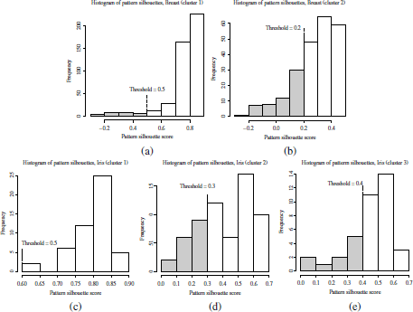
The specific criteria to select the silhouette thresholds can be illustrated by considering the clusters extracted from the iris and breast datasets (Figure 4.12). The distribution of silhouette scores has been estimated by using the histogram function in the R software, which also provides the vectors of silhouette values found as the histogram bin limits and the counts of occurrences in each bin.3 The silhouette thresholds have been selected to coincide with the histogram bin limits. In the breast dataset (two classes/clusters), the vector of silhouette thresholds for the first and second clusters is [0.5, 0.2]. The value silth = 0.5 for the first cluster corresponds to the upper bound ![]() as explained in the previous paragraph. This results in the removal of 5.2% of the cluster patterns. For the second cluster, the threshold silth = 0.2 is selected. The rejected section associated with silth corresponds to the first five histogram bins, comprising 25% of the patterns in the cluster. By including the sixth histogram bin in the pruned section, the next possible silhouette threshold level is silth = 0.3. However, such threshold level would lead to the removal of a considerable amount (46.28%) of the cluster patterns, which is considered unacceptable for preserving the cluster size/shape.
as explained in the previous paragraph. This results in the removal of 5.2% of the cluster patterns. For the second cluster, the threshold silth = 0.2 is selected. The rejected section associated with silth corresponds to the first five histogram bins, comprising 25% of the patterns in the cluster. By including the sixth histogram bin in the pruned section, the next possible silhouette threshold level is silth = 0.3. However, such threshold level would lead to the removal of a considerable amount (46.28%) of the cluster patterns, which is considered unacceptable for preserving the cluster size/shape.
A similar criterion has been followed for the clusters extracted in the iris dataset. The vector of cluster silhouette thresholds in this case is [0.5, 0.3, 0.4]. The first cluster is left unchanged by the pruning approach, as all observed silhouette scores exceed the upper bound ![]() . For the second cluster, a silhouette threshold silth = 0.3 has been selected, with an equivalent ratio of 27.42% of pruned patterns in the cluster. Note that, by including the next histogram bin (silth = 0.4), an inappropriate amount of patterns would be discarded (46% of the cluster size). Finally, the silhouette threshold for the third cluster is silth = 0.4 (26.31% of removed patterns), as the next possible silhouette level (0.5) would result in the removal of 55.26% of cluster patterns.
. For the second cluster, a silhouette threshold silth = 0.3 has been selected, with an equivalent ratio of 27.42% of pruned patterns in the cluster. Note that, by including the next histogram bin (silth = 0.4), an inappropriate amount of patterns would be discarded (46% of the cluster size). Finally, the silhouette threshold for the third cluster is silth = 0.4 (26.31% of removed patterns), as the next possible silhouette level (0.5) would result in the removal of 55.26% of cluster patterns.
To summarize, the number of histogram bins corresponding to rejected patterns is determined according to one of these two conditions:
– the upper limit of the last rejected bin should not exceed ![]() , and
, and
– the amount of rejected patterns (total number of occurrences in the rejected bins) should not exceed one-third of the total number of patterns in the cluster.
Another example of the pruned clusters on the mixtures of five and seven Gaussians is shown in Figure 4.13. The clusters obtained by the PAM algorithm have been tagged as C1 − C5 (five Gaussians) and C1 − C7 (seven Gaussians). Patterns rejected by the cluster pruning algorithm have been also indicated in red colors. The corresponding histograms of silhouette values are depicted in Figures 4.14 and 4.15. As can be observed, the mixture components in the five Gaussian datasets are well separated and thus easily identified by the clustering algorithm, which also provides well separated clusters. This can also be observed in the silhouette histograms in Figure 4.14. The minimum silhouette value observed in a majority of the clusters exceeds the upper bound for the silhouette threshold, ![]() . This means that all patterns in the clusters are preserved after cluster pruning. Only clusters C2 and C4 have both one pattern with silhouette scores lower than
. This means that all patterns in the clusters are preserved after cluster pruning. Only clusters C2 and C4 have both one pattern with silhouette scores lower than ![]() . Such patterns can be observed in red color in Figure 4.13(a). It can be observed that these patterns are outliers in their respective Gaussian components.
. Such patterns can be observed in red color in Figure 4.13(a). It can be observed that these patterns are outliers in their respective Gaussian components.
Figure 4.13. Example of patterns rejected by the cluster pruning approach in two mixtures of five and seven gaussians. The rejected patterns are indicated in red colors. (a) Five Gaussians; (b) seven Gaussians
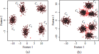
Figure 4.14. Histograms of silhouette values in the five Gaussians datasets, which were used for the determination of the clusters’ silhouette thresholds in the cluster pruning approach
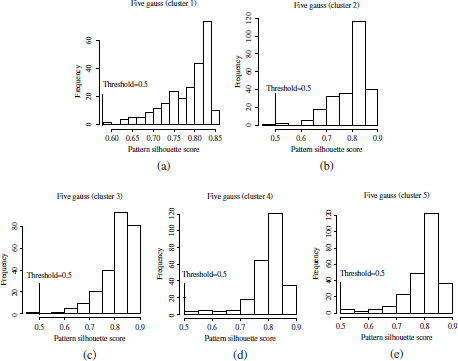
Figure 4.15. Histograms of silhouette values in the seven Gaussian datasets, which were used for the determination of the clusters’ silhouette thresholds in the cluster pruning approach. Shadow histogram bars correspond to the silhouette values of the rejected patterns

4.7.2. Evaluation of the cluster pruning approach
In this section, the efficiency of the cluster pruning method for rejecting misclassification errors from the clustered data is evaluated through an analysis of the algorithm outcomes on the iris, wine, breast cancer, diabetes, Pendig, and seven Gaussian datasets.4
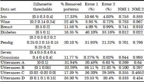
For the purpose of evaluating the cluster pruning algorithm, the cluster labeling task has been performed using the complete set of labels for each dataset. The resulting misclassification error rates as well as the NMI results observed in Table 4.1 confirm the adequate behavior of the cluster pruning algorithm for removing such sections from the clusters with a high probability of resulting misclassification errors after cluster labeling. For instance, while the pruned sections comprise around 10–20% of the patterns in the datasets, the percentage of remaining misclassification errors has been substantially reduced. As an example, the error rate has dropped from 10.66 to 4.03% after pruning on the iris data (62.2% error reduction), while error rate reductions of 75.8 and 92% have been attained on the breast and wine datasets, respectively. An exception to the previous observations is the diabetes dataset, in which the error rate after cluster pruning (38.16%) remains very similar to the original misclassification rate (40.10%). Note that, for two clusters, as in the case of the diabetes data, the worst possible error rate that can be observed is of 50%. Any error rate larger than 50% is not observed as it would just produces an inversion of the cluster labels. In other words, the original error in the diabetes dataset implies a roughly uniform distribution of patterns from any of the two underlying classes in the extracted clusters. This fact is also evidenced by the NMI score NMI=0.012. In consequence, the error rate is roughly the same after cluster pruning, and the removal of patterns by means of cluster pruning algorithm is just as efficient as removing the same amount of patterns at random.
Table 4.1. Some details about the cluster pruning approach in the Iris, Wine, Breast cancer, Diabetes, Pendig, Seven Gaussians and Utterances data sets
4.8. Simulations and results
In the experimental setting, SVMs have been used as the baseline classifier. First, each dataset has been divided into two training (~ 90%) and test (~ 10%) sets. In order to avoid possible biases of a single test set, such partition of the dataset has been randomly repeated to generate 20 different partitions. Also, for each one of these partitions, 20 different random seeds of labeled prototypes (n labels/category) have been selected. In total, 400 different prototype seeds (20 × 20) have been obtained. In the experiments, only prototype labels are assumed to be known a priori. No other class label knowledge has been applied to any of the algorithm stages. Each prototype seed has been used as the available training set for the supervised SVM. In the semi-supervised approach, these labeled prototype seeds have been used to trigger the automatic cluster labeling.
Both supervised and semi-supervised SVM classifiers have been evaluated on an accuracy basis, considering different number of labeled prototypes (samples) per category, from n = 1 to nmax = 30. The accuracy results obtained on the different datasets are shown in Figures 4.16–4.21. In particular, left plots are referred to the supervised and the semi-supervised approach without cluster pruning, while right plots are referred to the semi-supervised approaches by incorporating the cluster pruning approach. In all the cases, horizontal axes are referred to the sizes of the initial prototype seeds, whereas vertical axes indicate the mean accuracy scores, averaged over the 400 prototype initializations.
Figure 4.16. Comparison of the accuracy scores achieved by the supervised SVM and semi-supervised approach on the five Gaussian datasets. (a) Before cluster pruning; (b) after cluster pruning
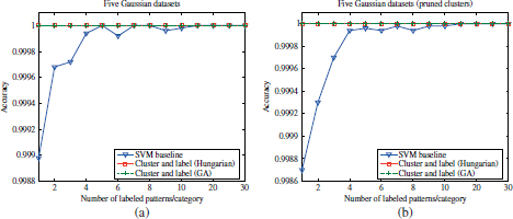
As can be observed in these Figures 4.17 and 4.21, the mean accuracy curves of the semi-supervised algorithm are roughly constant with the labeled set size. Only certain random variations can be observed, since the experiment outcomes for different seed sizes are referred to different random prototype seeds. However, it should be noted that, for each labeled set size, both supervised and semi-supervised outcomes have been simultaneously obtained with identical sets of prototypes, so that their respective accuracy curves can be compared. In contrast, the accuracy curves of the supervised approach show an increasing trend with the labeled set sizes. In the seven Gaussian, iris, Pendig, wine, and breast cancer datasets, the mean accuracy curves for the supervised and semi-supervised algorithms intersect at certain labeled set sizes, n′. For smaller labeled seed sizes (n < n′), the training “information” available in the augmented labeled sets (after cluster labeling) seems to be clearly superior than the the small labeled seeds. Therefore, although the augmented labels are not exempted from misclassifications due to clustering errors, higher prediction accuracies are achieved by the semi-supervised approach with respect to the supervised classifier. For (n > n′), the information in the increasing labeled seeds compensates for the misclassification errors present in the augmented sets and thus the supervised classifier outperforms the semi-supervised approach. As shown in the previous section, these errors present in the augmented datasets can be notably reduced by means of cluster pruning. Consequently, an improvement in the prediction accuracies achieved by the semi-supervised algorithm is generally observed by incorporating the cluster pruning algorithm (Figures 4.16b; 4.17b; 4.17 and 4.18b; 4.18 and 4.19b; and 4.19).
Figure 4.17. Comparison of the accuracy scores achieved by the supervised SVM and semi-supervised approach on the seven Gaussian and Pendig datasets. (a and c) Before cluster pruning; (b and d) after cluster pruning

Figure 4.18. Comparison of accuracy scores achieved by the supervised SVM and semi-supervised approach on the iris and breast datasets. (a and c) Before cluster pruning; (b and d) after cluster pruning

Figure 4.19. Comparison of accuracy scores achieved by the supervised SVM and semi-supervised approach on the wine and Diabetes datasets. (a and c) Before cluster pruning; (b and d) after cluster pruning
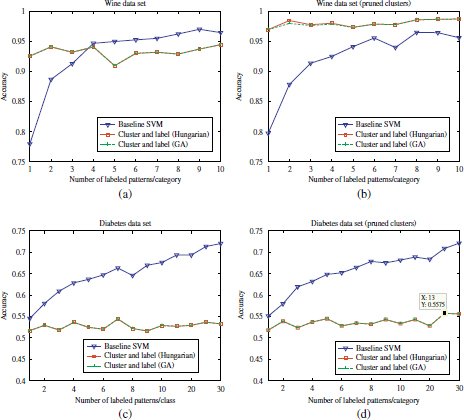
Unlike the accuracy results observed in the seven Gaussian, iris, Pendig, Wine, and breast cancer datasets, a degradation in the semi-supervised classification performance with respect to the supervised classifier is observed in the diabetes dataset, regardless of the initial labeled seed sizes. This observation is strictly associated with the NMI scores of the extracted clusters presented in the previous section (NMI=0.012), which corresponds to a misclassification rate of 40.10%. This means that almost no information concerning class labels is present in the augmented datasets used to train the SVM models. The semi-supervised performance on the diabetes dataset is thus comparable to the trivial classifier. In other words, the main condition for cluster and label approaches — the patterns in a dataset should naturally fall into clusters — is not fulfilled in the diabetes dataset (using the PAM clustering algorithm).
Figure 4.20. Comparison of accuracy scores achieved by the supervised and semi-supervised approaches in a data set of utterances (2 classes). (a) and (c): before cluster pruning (b) and (d): after cluster pruning

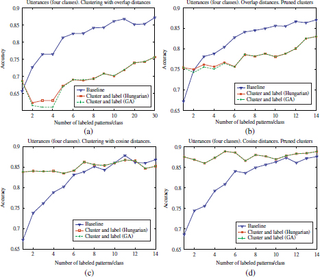
Figure 4.21. Comparison of accuracy scores achieved by the supervised and semi-supervised approaches in a data set of utterances (4 classes). (a) and (c): before cluster pruning (b) and (d): after cluster pruning
4.9. Summary
In this chapter, a semi-supervised approach has been presented based on the cluster and label paradigm. In contrast to previous research in semi-supervised classification, in which labels are commonly integrated in the clustering process, the cluster and labeling processes are independent from each other in this work. First, a conventional unsupervised clustering algorithm, the PAM, is used to obtain a cluster partition. Then, the output cluster partition as well as a small set of labeled prototypes (also refered to as labeled seeds) is used to decide the optimum cluster labeling related to the labeled seed. The cluster labeling problem has been formulated as a typical assignment optimization problem, whose solution may be obtained by means of the Hungarian algorithm or GA. Experimental results have shown significant improvements in the classification accuracy for minimum labeled sets, in such datasets where the underlying classes can be appropriately captured by means of unsupervised clustering.
In addition, an optimization of the semi-supervised algorithm has been also developed by discarding the patterns clustered with small silhouette scores. Thereby, it has been shown that the quality of the pruned clusters can be improved, as significant reductions in the misclassification errors present in the clustered data are achieved through the removal of relatively small amounts of patterns from the clusters.
Future work is to analyze further alternatives for the definition of the cost matrix used by the Hungarian algorithm. Currently, the cost matrix is based on a number of (labeled) patterns from each class that are observed in the clusters. Hence, the Hungarian algorithm provides the solution with the maximum overlapping of clusters and class labels. However, if an inappropriate labeled seed contains a large amount of patterns from class overlapping regions, the optimum solution based on such labeled seed may result in cluster labeling errors (i.e., two or more clusters may be assigned to a different class label to the one which is generally represented by the patterns in the cluster). Obviously, in these situations, the amount of misclassification errors in the augmented datasets leads to incorrect learned models and false predictions concerning the erroneous class labels. This problem may be palliated, for example, through a new probabilistic definition of the cost matrix, by estimating, for each class, the conditional probabilities of the clusters given the class’ labels in the initial seeds.
1. Although class labels can take any arbitrary value, either numeric or nominal, for simplicity in the formulation and implementation of the cluster labeling problem the k class labels are transformed into integer values ([1,…,k])
2. The term missclasification is not used here to indicate the predicted errors of the end classifiers but the errors after the cluster labeling block. Note that, after cluster labeling, each clustered data pattern has been assigned a class label (the label of its cluster), which can be compared with the real label if the complete labeled set is available.
3. The bin sizes provided by the R software histogram function are estimated according to the Sturges formula [FRE 81].
4. Note that the cluster partitions obtained in there experiments comprise all instances of the datasets (without prior partitions into test/training).