
Chapter 3
Semi-Supervised Classification Using Prior Word Clustering
3.1. Introduction
In the first part of this book, two semi-supervised approaches have been developed, which exploit the availability of unlabeled data by means of unsupervised clustering.
As stated in Chapter 1, cluster and label approaches in the machine learning literature often merge the cluster and label steps as a global optimization problem in which both tasks are simultaneously solved. The approaches developed in this book are intended to avoid the influence of the labeled seeds on the cluster solution, which can induce wrong clustering if potential labeling errors are present in the labeled sets.
In particular, the algorithm described in this chapter is based on the synonymy assumption: under minimal class labels, the underlying classes can be approximately recovered by extracting semantic similarities from the data. The synonymy assumption has been applied to the feature space in which a clustering algorithm is used to extract groups of synonym words. In previous research [LI 98], word clustering has been typically investigated as a feature clustering strategy for supervised text classification. By applying word clustering for supervised classification, a degradation in the classification accuracy was reported. However, in the experiments described in this chapter, it is shown that a classification algorithm using minimum labeled seeds can benefit from word clustering on unlabeled data (semi-supervised classification).
Furthermore, besides the use of unlabeled data for word clustering, unlabeled data has also been used for unsupervised disambiguation of ambiguous utterances.
3.2. Dataset
The approaches described in the following have been applied to a collection of utterance transcripts. In particular, the utterance dataset from the video troubleshooting domain has been selected (see section 1.1 in Chapter 1).
3.3. Utterance classification scheme
The supervised utterance classification scheme is depicted in Figure 3.1. First, each utterance is pre-processed into an utterance vector. The classification algorithm then maps this vector into one of the categories from the list of symptoms. The pre-processing step and classification algorithm are described in detail in sections 3.3.1 and 3.3.2.
3.3.1. Pre-processing
As mentioned earlier, the pre-processing step transforms each input utterance transcript ui into an utterance vector xi, which is the utterance form used by the classification algorithm. The first pre-processing step extracts the surface form of the utterance words. As introduced in Chapter 1, a possible surface form of a word is the word’s stem. However, after word stemming, the lexical category of the original word is not preserved. For example, the following utterances
Figure 3.1. Supervised utterance categorization scheme using the NN algorithm
“need a worker to install Internet” [Appointment]
“have installed Internet but it does not work” [Internet]
would lead, after stop-word removal, to very similar bag-of-words vectors if the word worker were reduced to its stem form work. However, the utterances have been annotated with different categories ([appointment] and [Internet], respectively). For this reason, a lemmatizer [TOU 00] has been selected instead (note that the lemma form of worker remains worker).
Following the lemmatizing step, stop-word filtering has been applied. It discards ubiquitous terms deemed irrelevant for the classification task as they do not contribute any semantic content to the utterances. Examples are the lemmas a, the, be, and for. In this book, the SMART stop list has been used [SAL 71] with small modifications. In particular, confirmation terms (yes, no) have been deleted from the stop-word list, whereas words typical for the spontaneous speech (eh, ehm, uh, …) have been introduced as stop words.
As an example of the transformation of utterances and words through the pre-processing steps, the input utterance My remote control is not turning on the television is transformed as follows:
Utterance (ui): “My remote control is not turning on the television”
+ Lemmatizing ![]() : “My remote control be not turn on the television”
: “My remote control be not turn on the television”
+ Stop-word filtering ![]() : Remote control not turn television
: Remote control not turn television
where the notations ui, ![]() , and
, and ![]() refer to the initial utterance transcript, the utterance after lemmatizing (l), and the utterance after lemmatizing and stop-word filtering (l+s).
refer to the initial utterance transcript, the utterance after lemmatizing (l), and the utterance after lemmatizing and stop-word filtering (l+s).
3.3.1.1. Utterance vector representation
The salient vocabulary or lexicon is obtained after preprocessing all utterances in the training corpus, ![]() T. The lexicon
T. The lexicon ![]() = {w1,w2,…,wD} is then defined as the set of different lemmas found in the pre-processing training set. In the following, the lexicon elements are also referred to as terms. The number of terms extracted from the Internet corpus is D = 1,614. Finally, a binary vector model (“bag-of-words”) has been selected to represent the pre-processed utterances,
= {w1,w2,…,wD} is then defined as the set of different lemmas found in the pre-processing training set. In the following, the lexicon elements are also referred to as terms. The number of terms extracted from the Internet corpus is D = 1,614. Finally, a binary vector model (“bag-of-words”) has been selected to represent the pre-processed utterances,
where xi denotes an utterance vector. As already explained for texts, each binary element ![]() indicates the presence or absence of the term wi in the pre-processed utterance transcript,
indicates the presence or absence of the term wi in the pre-processed utterance transcript, ![]() :
:
3.3.2. Utterance classification
A simple yet robust categorization approach is the nearest neighbor (NN) algorithm (j-NN). Let ![]() denote the labeled seed of prototype vectors and K the set of k possible class labels. The j-NN algorithm compares each input utterance vector xi to its closest j prototype vectors (nearest neighbors) and decides the most frequent category in the NNs according to a majority voting criterion. In this work, the labeled seed is composed of one prototype per category (n= 1). Thus, the j-NN algorithm derives into a simple 1-NN rule. The NN classification rule, θNN, decides for each input utterance vector in a test set, xi ∈
denote the labeled seed of prototype vectors and K the set of k possible class labels. The j-NN algorithm compares each input utterance vector xi to its closest j prototype vectors (nearest neighbors) and decides the most frequent category in the NNs according to a majority voting criterion. In this work, the labeled seed is composed of one prototype per category (n= 1). Thus, the j-NN algorithm derives into a simple 1-NN rule. The NN classification rule, θNN, decides for each input utterance vector in a test set, xi ∈ ![]() (test), the symptom category of the closest prototype vector:
(test), the symptom category of the closest prototype vector:
In this work, the overlap distance has been applied to compute the dissimilarities between utterance vectors. First, the overlap similarity between two utterance vectors is the number of words that overlap in the pre-processed utterances. This metric of similarity is equivalent to the dot product between utterance vectors:
The overlap distance can be calculated as the inverse of the overlap dissimilarity:
[3.4] ![]()
Note that the prototype vectors applied to the NN algorithm have been manually selected. In this work, the basic criterion for the selection of the prototype set ![]() is the minimum possible term overlap between different prototypes in the codebook.
is the minimum possible term overlap between different prototypes in the codebook.
3.4. Semi-supervised approach based on term clustering
In this section, a semi-supervised version of the utterance classification scheme in Figure 1.1 is introduced. By applying a unique labeled utterance per category, a poor classification performance is to be expected, in comparison with other classifiers with large labeled prototype seeds. One reason for this poor performance can be explained by the prevalence of certain language effects such as synonymy and polysemy, which are not sufficiently covered in the minimum labeled seed. Synonymy refers to the capability of language to describe a single semantic concept with different words (synonym). Polysemy, however, is the use of a unique word form with multiple meanings.
The synonymy effect is patent in the effective vocabulary available to the classifier, which is reduced to less than 5% of the total vocabulary dimension in ![]() . This results in a large amount of utterances mapped to a [nomatch] class, given the existence of out-of-vocabulary terms in the test utterances.
. This results in a large amount of utterances mapped to a [nomatch] class, given the existence of out-of-vocabulary terms in the test utterances.
As an example, one of the symptom categories, [NoSound], represents the problems related to sound. A prototypical caller utterance reporting this problem is “No sound.” However, the user may speak other alternatives, such as “problem with volume” or “lost audio,” which are not matched against the mentioned prototype (no sound) due to the orthogonality between their vectors. In other words, there are no overlapping terms between the input utterances and the prototype utterance. This problem can be partially solved using the observation that sound has a similar meaning as that of audio or volume.
Given these statements, a feature extraction technique that identifies groups of terms on the basis of the semantic affinities among them has been developed in this work. Synonym terms are identified from a training set composed of both labeled and unlabeled data:
where ![]() refers to the labeled seed (prototypes) and
refers to the labeled seed (prototypes) and ![]() indicates the unlabeled portion of
indicates the unlabeled portion of ![]() T . Thus, the new algorithm may be considered as a semi-supervised version of the basic classification scheme as shown in Figure 3.1. A similar approach was made in the literature [DEP 00], in which a list of manually selected keywords and their synonyms was used to trigger an unsupervised classification of texts. In this work, a method to automatically extract classes of semantically related words from the corpus of utterance transcripts has been developed.
T . Thus, the new algorithm may be considered as a semi-supervised version of the basic classification scheme as shown in Figure 3.1. A similar approach was made in the literature [DEP 00], in which a list of manually selected keywords and their synonyms was used to trigger an unsupervised classification of texts. In this work, a method to automatically extract classes of semantically related words from the corpus of utterance transcripts has been developed.
Although a number of manually compiled word thesauri are available nowadays, such as Wordnet [WOR 98], the automatic identification of related words provides certain advantages over manually constructed thesauri. The most important one is that automatic methods can be better adapted to a specific domain, as they are statistically “trained” on specific data. As an example, the words confirm and schedule are not apparently synonym terms. However, on the Internet corpus, both terms are strongly related to the category [Appointment]. Typical user utterances for this category are, for example, “I want to confirm an appointment” and “I want to schedule an appointment.” Furthermore, both terms have barely any occurrences outside the [Appointment] category.
The block diagram of the new semi-supervised algorithm with term clustering can be seen in Figure 3.4.
3.4.1. Term clustering
The automatic identification of semantic term classes is performed in two main steps:
Figure 3.2. Utterance categorization using the NN algorithm and a term clustering scheme as feature extraction. To address the synonymy problem, a hard clustering scheme can be used. It performs a unique mapping of each term in the vocabulary into a single semantic class. Another possibility is to use fuzzy algorithms to provide a fuzzy or soft association of each term pattern to the output semantic classes through a membership matrix. The association of hard clustering is represented in the figure as bold traces, whereas a fuzzy association is denoted as thin lines
– the definition of distance metrics that allow us to capture semantic dissimilarities between the terms; and
– the application of a clustering scheme to the matrix of dissimilarities obtained from Step 1.
Both tasks are described in detail in sections 3.4.2 and 3.4.4.
3.4.2. Semantic term dissimilarity
As mentioned earlier, the first task related to the extraction of synonym terms through clustering approaches is the calculation of dissimilarity matrices that reflect the semantic differences between the terms.
For that purpose, in a similar way as utterances have been represented in the bag-of-words vectors, an encoding of terms in vector structures has been applied. This allows for the comparison of terms in a vector space.
3.4.2.1. Term vector of lexical co-occurrences
As an attempt to explain the main characteristics of semantically related terms two basic criteria have been proposed in the literature:
– First-order co-occurrence: two words are semantically similar to the degree that they show patterns of co-occurrence and co-absence in the same texts [WUL 97].
– Second-order co-occurrence: two words are semantically similar to the degree that they occur in the neighborhoods of similar words [PIC 99].
The first-order co-occurrence criterion is adequate for text documents, as synonym words are expected to co-occur in the same document. In contrast, semantically related words are not expected to co-occur inside an utterance transcript or sentence, as the semantic variability of a sentence is substantially reduced in comparison to text documents. This fact is also shown in the Internet corpus of utterances. For example, in the category [Operator], the synonym terms speak and talk are typically “exclusive” inside utterances, such as “I want to talk to an operator” or “I want to speak to an operator.” However, the second-order co-occurrence criterion is adequate for capturing their semantic connection, as the terms usually occur with similar contexts1 (e.g. the terms operator, representative, and agent).
Consequently, each term in the vocabulary, wi ∈ W, has been defined as a D-dimensional vector:
[3.6] ![]()
whose components indicate the relative frequency of occurrence of the term ωi in the same utterances with the other D−1 terms in the vocabulary:
where N(wi,wj) denotes the total number of times that ωi and ωj co-occur.
As an example, the co-occurrence vector for the word operator (for occurrence frequencies larger than 0) is the following:
C[operator](%): need(15%), talk(11.2%), speak(10.3%), please(9.9%), want(5.1%), give(3.8%), get(2.5%), date(1.7%), help(1.7%), agent(1.7%), Internet(1.7%), human(1.2%), real(1.2%), let(1.2%), service(1.2%), not(1.2%), id(0.8%), technical(0.8%), line(0.8%).
3.4.2.2. Metric of dissimilarity
Given the term vector representation, one of the popular distance functions which can be used to compute the dissimilarities between term vectors is the Euclidean distance:
However, one important observation using the Euclidean distance is that relevant terms, occurring in the same contexts of the terms that are to be compared, contribute more significantly to the distance between the terms. This fact can be illustrated with the utterance vectors for the terms talk and speak (Table 3.1).
Table 3.1. Comparison of the terms ωi (talk) and ωj (speak) — table rows. The term that occurs more often in their neighborhoods is agent (first column). However, by applying the Euclidean distance, this term contributes a significant increment to the total distance between talk and speak in comparison with other terms in the table columns

As can be observed, the word with the highest co-occurrence patterns with the terms talk and speak is agent. However, the contribution of this term to the total distance deuc(talk, speak) is ((0.2 - 0.18)2 = 0.0004). This value is substantially larger than the contributions of other terms with occasional cooccurrences in the contexts of talk and speak. For example, the contribution due to the term give is (0.003-0.001)2 = 0.000004.
Therefore, a normalization of the Euclidean distance has been defined, according to the following equation:
[3.9] 
The larger the value of the minimum min![]() , the more important is the term wk to explain the similarities between wi and wj. Thus, a higher normalization score in this case decreases the distance between the terms wi and wj.
, the more important is the term wk to explain the similarities between wi and wj. Thus, a higher normalization score in this case decreases the distance between the terms wi and wj.
3.4.3. Term vector truncation
An extension of the term vector definition in equation [3.6] was motivated by the different patterns of co-occurrences and their subsequent effects on the semantic term dissimilarities. As suggested in section 3.4.2, while a few terms “explain” the semantic behavior and affinity of two terms ωi and ωj being compared, many other terms show occasional occurrences with these terms. This observation in the term (co-occurrence) vectors can be interpreted as an underlying noise pattern with a certain impact in the calculation of distances.
In consequence, a new term co-occurrence vector has been defined,
[3.10] ![]()
by setting a minimum co-occurrence threshold Nth = 1%. Such words, wk, whose co-occurrence value in the word vector wi do not exceed this minimum co-occurrence threshold have been considered as “noise words” and were discarded from the original term vector.
Then, the new co-occurrence values have been then recalculated so that the co-occurrence values ![]() build another random variable, i.e.
build another random variable, i.e. ![]() . The new vector can be formulated as follows:
. The new vector can be formulated as follows:
[3.11] 
As can be observed, the important co-occurrences in wi are placed with higher emphasis with respect to the original vector. As an example, the co-occurrence vector for the term Operator is modified as follows:
C[operator](%): need(15%), talk(11.2%), speak(10.3%), please(9.9%), want(5.1%), give(3.8%), get(2.5%), date (1.7%), help(1.7%), agent(1.7%), Internet(1.7%), human(1.2%), real(1.2%), let(1.2%), service(1.2%), not(1.2%), id(0.8%), technical(0.8%), line(0.8%),…
after term vector truncation:
C[operator](%): need(21.24%), talk(15.86%), speak (14.59%), please(14.02%), want(7.22%), give(5.38%), get(3.54%), date(2.41%), help(2.41%), agent(2.41%), Internet(2.41%), human(1.69%), real(1.69%), let(1.69%), service(1.69%), not(1.69%).
3.4.4. Term clustering
Finally, a clustering algorithm has been applied to the matrix of term dissimilarities (equation [3.9]) to extract clusters of similar terms. By denoting ![]() , the set of synonym term clusters, a “hard” clustering algorithm is equivalent to an implicit mapping function Fc that uniquely maps each lexicon term to one of the clusters in
, the set of synonym term clusters, a “hard” clustering algorithm is equivalent to an implicit mapping function Fc that uniquely maps each lexicon term to one of the clusters in ![]()
In this work, the clustering algorithm that extracts semantic clusters is based on the complete link criterion for merging a pair of candidate clusters. As described in Chapter 1, the complete link clustering algorithm requires all elements in a cluster to be less distant from each other than the threshold distance specified by the user. The reason for the selection of the complete link merging criterion is that all (synonym) words inside a cluster should be strictly related to each other. However, the implemented clustering algorithm differs from the complete linkage clustering in the selection for the next pair of clusters to be merged at the next step. This is based on a single link criterion (the clusters with the closest patterns are selected instead). The algorithm is described in the following steps:
1. Input: Matrix of dissimilarities between the terms.
2. Output: Set of word clusters of semantically related words, S = {S1, S2, …, Sk}.
3. Initialization: Place each term wi in its own cluster: Si = {wi}.
4.Find the terms wi and wj with minimum distance, dmin in the similarity matrix.
4.1.Merging step: If the terms wi and wj, which are found in Step 4, belong to different clusters, ![]() , and the distance of the farthest elements in ca and cb is lower than the specified threshold distance, dth (dmax(ca, cb) ≤ Dth) merge clusters ca and
, and the distance of the farthest elements in ca and cb is lower than the specified threshold distance, dth (dmax(ca, cb) ≤ Dth) merge clusters ca and
4.2.Update dissimilarity matrix, so that dij = dji = ∞.
5. Repeat from Step 4 until all terms remain assigned to a single cluster or no pair of terms, wi and wj, can be found whose clusters are less distant than Dth.
As shown in Figure 3.2, the clustering solution can be represented as a binary membership matrix, M[DxD′].
![]()
where each binary element M[i, j] denotes the “hard” membership of the input lexicon term wi in the output semantic cluster Sj.
Tables 3.2 and 3.3 show two examples of the semantic clusters (with more than one member) obtained by the term clustering algorithm with dth = 0.3 and 0.5. An observation from these tables explains the relationships of the terms inside each extracted cluster. The major objective of term clustering was to identify semantically related terms, which co-occur with similar contexts due to their semantic equivalence. Thus, they can replace each other in an utterance with no semantic change. Good examples of synonyms successfully identified by the algorithm are the pairs (speak, talk), (somebody, someone), (mail, Email), and (website, site). However, not only synonym terms have been identified by the algorithm. Other meaningful components that have been also extracted as a “side product” are frequent term bi-grams. In contrast to uni-grams, bi-grams are pairs of consecutive words (w1,w2) whose high co-occurrence pattern evidences significant conditional statistical dependencies, i.e. P(w2|w1) ≥ P(w2). Some examples are the pairs (technical, support), (antivirus, security), (parental, control), (error, message), and (user, name). This observation is related to the definition of words in term vectors of term co-occurrences. In fact, a bi-gram pair of terms that co-occur frequently in the training corpus should have close co-occurrence vectors. This happens because the words that occur in the contexts of both bi-gram terms are also similar.
Table 3.2. Example of classes of semantically related terms extracted with a clustering threshold distance dth = 0.3
| Semantic classes (example with threshold distance 0.3) |
| talk speak agent customer representative support tech operator human person someone somebody security suite user name email mail outlook website site virus protection cancel schedule date ping quality picture sound software c-d parental control i-p d-n-s box converter error message cancel schedule date connect run modem router trouble network system p-c figure speed company installation pipeline d-s-l kit cable t-v line receive check computer information channel homepage turn see service phone hook put say keep signal response |
Table 3.3. Example of classes of semantically related terms extracted with a clustering threshold distance dth = 0.5
| Semantic classes (example with threshold distance 0.5) |
| talk speak operator human agent customer representative support person tech website site email mail outlook signal parental control security suite virus protection page webpage error message program software c-d antivirus someone technical somebody installation assistance pipeline channel homepage cancel schedule date make confirm help setup buy purchase question user name i-p ip d-n-s receive send check box converter Microsoft d-s-l kit router laptop Ethernet go tell install call say keep use put hookup set add connect hook run start firewall domain screen light know reconnect mailbox configuration service phone day turn see download scan come disconnect leave something card yahoo game m-s-n house room net code disk communication web a-o-l |
3.4.5. Feature extraction and utterance feature vector
By applying clustering of semantic classes, the utterance vector needs to be redefined with the new extracted features (semantic classes). Given S, the set of semantic clusters extracted through the term clustering scheme, and M, the cluster membership matrix that encodes the term clustering output, the feature extraction that transforms the input utterance vector xi into a vector of semantic features ![]() is defined as follows:
is defined as follows:
In other words, each binary component of the utterance feature vector ![]() denotes the presence/absence of at least one member of the semantic cluster Sj in the pre-processed utterance
denotes the presence/absence of at least one member of the semantic cluster Sj in the pre-processed utterance ![]() .
.
3.4.6. Evaluation
The symptom categorization of user utterances has been evaluated on an accuracy basis. The accuracy achieved by the classification algorithm is calculated by comparing the automatic symptoms (labels) assigned by the algorithms to the input test utterances with the corresponding manual labels, which are available for test purposes. The accuracy is then defined as the ratio of correctly classified utterances over the total number of utterances in the test set:
Although typical evaluation criteria used for the categorization of texts are the microaverage F metrics, but in this work, the accuracy has been preferred to the microaverage metric. In fact, accuracy scores have been considered as a better indicator of the percentage of correctly routed calls due to the symptom categorization module of the Spoken Language Dialogue Systems (SLDS).
Note that the microaverage F1 corresponds to the accuracy of uniformly distributed classes. However, for skewed distributions, a classifier may produce high accuracy values but low F1 scores. This occurs when a high ratio of the correct classifier predictions are concentrated in the most frequent classes. In this work, since a frequent class indicates a frequent reason for calls, high accuracy values are still good indicators for the average performance of the SLDS. First, the performance of the supervised classification algorithm (Figure 3.1) has been compared with the semi-supervised classification using term clustering. Some examples of the accuracy results obtained with six different labeled seeds initializations are shown in Figures 3.3–3.5. The vertical axes refer to the accuracy scores, whereas the horizontal axes indicate different distance thresholds applied to the term clustering algorithm for the semi-supervised approach.
Figure 3.3. Comparison of accuracy scores of the supervised classifier versus the semi-supervised approach with term clustering, using two different initializations
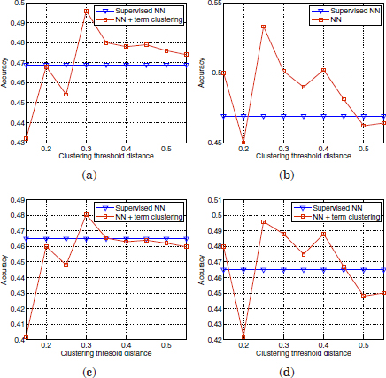
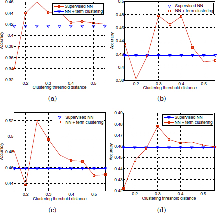
Each pair of plots 3.3(a,b), 3.3(c,d), 3.4(a,b), 3.4(c,d), 3.5(a,b), and 3.5(c,d) are referred to identical labeled seeds. The difference in the left plots with respect to the right plots is the term vector representation applied to the term clustering in the semi-supervised approach. The left plots are referred to the basic term vector definition in equation [3.11], whereas the right plots are referred to the term vector definition after truncation (equation [3.10]).
Figure 3.4. Comparison of accuracy scores of the supervised classifier versus the semi-supervised approach with term clustering, using two different initializations
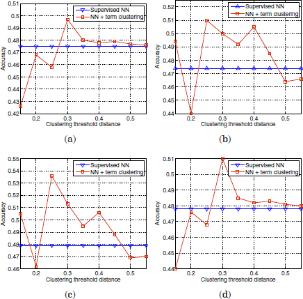
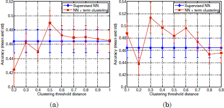
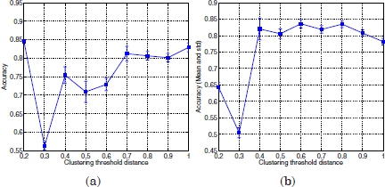
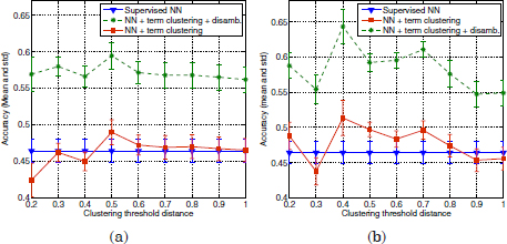
Figure 3.6 shows the mean accuracy values of the supervised and semi-supervised classification schemes over 20 different prototype labeled seeds initializations. Standard deviations are indicated as shadowed areas around their respective mean curves. Figure 3.6a shows the classification accuracy of the supervised scheme and the semi-supervised approach using the term vector definition of equation [3.11]. Figure 3.6b refers to the term vector definition in equation [3.10]. Although the performance of the semi-supervised classifier depends on the threshold distance dth applied to term clustering, some improvements can be observed for different values dth, up two 2%, using the definition of a term co-occurrence vector in equation [3.11] and 5.5% if word vector truncation is applied.
Figure 3.5. Comparison of accuracy scores of the supervised classifier vs. the semi-supervised approach with term clustering, using two different initializations
3.5. Disambiguation
If applied to utterance bag-of-words or feature vectors, the NN classifier rejects a considerable number of ambiguous utterances for which several candidate prototypes are found. Candidate prototypes are labeled utterance vectors in ![]() , which share maximum proximity to the input utterance. This happens especially when the similarity metric between the vectors results in integer values, as the overlap distance in equation [3.4]. A disambiguation module (Figure 3.7) has therefore been devised to resolve the mentioned ambiguities and to map an ambiguous utterance to one of the output categories.
, which share maximum proximity to the input utterance. This happens especially when the similarity metric between the vectors results in integer values, as the overlap distance in equation [3.4]. A disambiguation module (Figure 3.7) has therefore been devised to resolve the mentioned ambiguities and to map an ambiguous utterance to one of the output categories.
Figure 3.6. Mean accuracy values over 20 labeled seeds initializations achieved by the supervised NN classifier vs. the semi-supervised approach with term clustering. Standard deviations are indicated as shadowed areas around their respective mean curves. (a): Supervised NN based on bag of words features vs .semi-supervised using semantic class features. (b): Supervised vs. semi-supervised by incorporating word vector truncation
First, the terms that cause the ambiguity are identified and stored in a list of competing terms. As an example, consider the utterance I want to get the virus off my computer. After pre-processing and hard term clustering, this utterance results in the feature set computer get off virus. The feature vector has minimum distance to the prototypes computer freeze [CrashFrozenComputer] and install protection virus [Security]. The competing terms that produce the ambiguity are in this case the words computer and virus. Therefore, in this study, the disambiguation among prototypes (or categories) is equivalent to a disambiguation among competing terms. For this reason, as a further means of disambiguation, the informativeness of a term wi has been estimated as shown in equation [3.15]:
Figure 3.7. Disambiguation scheme used for utterance categorization
[3.15] 
where Pr(wi) denotes the maximum-likelihood estimation for the probability of the term wi in the training corpus, and Lj refers to the part of speech (POS) tag of wj, where N refers to nouns. POS tags have been extracted by means of the Standford POS tagger [TOU 00].
As can be inferred from equation [3.15], two main factors are taken into account to estimate the relevance of a word for the disambiguation:
– the word probability and
– the term co-occurrence with frequent nouns in the corpus.
The underlying assumption that justifies this second factor is that words representative of problem categories are mostly nouns and appear in the corpus with moderate frequencies. The parameter α is intended to control the trade-off between the two factors. Reasonable values are in the range of (α ∈ [1,2]) placing some emphasis on the second factor; a value of α = 1.6 has been selected in the experiments, although other values in the mentioned range may yield a similar performance.
Finally, the term with the highest informativeness is selected among the competitors, and the ambiguous utterance vector is matched to the corresponding prototype or category.
3.5.1. Evaluation
The disambiguation scheme has been also individually evaluated. For this purpose, two cases of ambiguous utterances need to be distinguished:
(a) resolvable ambiguities: ambiguous utterances that can be resolved using the disambiguation scheme because one of their “candidate prototypes” corresponds to the true (manual) category of the input utterance and
(b) unresolvable ambiguities: ambiguous utterances that cannot be resolved, because no candidate prototype corresponds to the category of the utterance; thus, no disambiguation strategy can be applied in this case.
To assess the disambiguation performance of the disambiguation scheme, only resolvable ambiguities have been considered. A resolvable ambiguity is said to be “correctly resolved,” if the winning prototype is the one with the same category as the manual category of the utterance. The disambiguation accuracy is then formulated as follows:
Disambiguation accuracies
Figure 3.8 shows the mean disambiguation accuracy of ambiguous utterance vectors over 20 different prototype initializations, with respect to the variable dth used in the term clustering algorithm. Figure 3.8a refers to the basic term clustering strategy without vector truncation. Figure 3.8b corresponds to term clustering and term vector truncation.
Figure 3.8. Disambiguation accuracies obtained by the disambiguation scheme. (a): using term Clustering, (b): term clustering and term vector truncation
As can be observed, the disambiguation performance varies with the values of dth used in the term clustering algorithm. It reaches a minimum accuracy score at dth = 0.3, both with and without vector truncation. From this point, it shows an increasing trend with the dth variable, which is more abrupt if vector truncation is applied before term clustering. This trend in the disambiguation performance is strongly associated with the clustering scheme (see Figure 3.9).
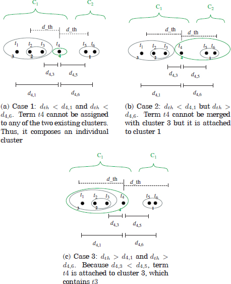
Ideally, each extracted cluster should be composed of terms that are mostly relevant for a topic category. However, as illustrated in Figure 3.9c (case 2), certain values of dth produce clusters of terms descriptive for different categories. For example, terms t1-t4 in the figure are assumed to be relevant for a certain topic category, C1. Likewise, terms t5 and t6 are assumed to be representative for a second category, C2. The order in which clusters are extracted by the algorithm is denoted by the labels (1–4). Terms t1,t2,t3,t5 and t6 are allocated in clusters 3 and 4 in all three cases. These allocations correspond to their relevant categories, C1 and C2. In contrast, different cluster allocations can be found for the term t4, depending on dth. If the value of dth is too small (case 1), the complete link criterion is not fulfilled for any of the two existing clusters and t4 composes an individual cluster. A small increase in dth such that t4 only satisfies the merging criterion for cluster 1 causes the term t4 to be attached to such cluster (case 2). This situation can lead to an increment in ambiguous utterances due to a possible overlapping of terms in some of the labeled prototypes. A further increment in dth, such that d4 1 ≤ dth (the merging condition for both clusters 1 and 3 is fulfilled) allows the attachment of t4 to cluster 1. t4 is not assigned to cluster 1 because the single link search criterion of this cluster algorithm gives the priority to cluster 3 (as d4,3 < d4,5). In this situation, the cluster configuration is consistent with the (real) sets of descriptive terms for the categories C1 and C2.
Figure 3.9. Illustration of term clustering with different values of the threshold distance with an hypothetical uni-dimensional example
The previous explanation can also be associated with the true semantic clusters extracted by the term clustering algorithm. Case 2 in Figure 3.9 is equivalent to the cluster output for dth = 0.3 (Table 3.2). The terms router and modem are allocated into the same cluster by the term clustering algorithm. However, these terms commonly occur with different topic categories, [Homenetwork] and [Modem], respectively. Typical utterances for the mentioned categories are “wireless router” and “modem.” They are often applied as the labeled prototypes for these categories. Since modem is the most frequent term in the cluster, it is selected as the cluster’s representative term. Thus, the prototypes after term clustering are (wireless modem) and (modem). Any input utterance whose bag-of-words vector only overlaps modem or router with the prototypes results in an ambiguous vector, as both terms derive into a single cluster representative (modem). Since the categories [modem] and [homenetworks] occur with relatively high frequencies, this “error” in term clustering yields a significant amount of ambiguities, as shown in Figure 3.10. Furthermore, although such an ambiguous utterance may be a resolvable ambiguity as defined earlier, it cannot be resolved by the disambiguation scheme since the conflictive terms are “identical” (modem). In other words, the term’s informativeness criterion is not sufficient to discriminate among prototypes. In these cases, the decision for the winning category is randomly performed. As can be observed in Figure 3.10, while the number of ambiguities considerably increases for dth = 0.3, only a small increment is attained on the number of ambiguities correctly resolved.
Figure 3.10. Number of ambiguous patterns found by the utterance classification scheme. (a): with term clustering, (b): with term clustering and term vector truncation
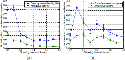
Figure 3.11. Comparison of accuracy scores of the supervised
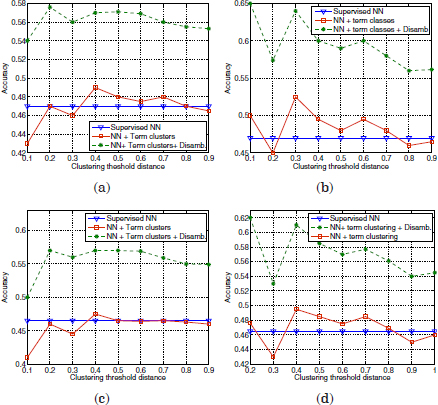
Final accuracy scores of the semi-supervised classification before and after disambiguation versus the supervised classification can be observed in Figures 3.11–3.13. As in section 3.4.6, the semi-supervised evaluation in these figures is referred to six different labeled seed initializations. The left plots in these figures are referred to the basic term vector definition in equation [3.11], whereas the right plots are referred to the term vector definition after truncation (equation [3.10]).
Figure 3.12. classifier vs. the semi-supervised approach before and after disambiguation using two different prototype initializations
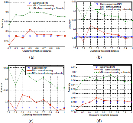
Figure 3.13. Comparison of accuracy scores of the supervised
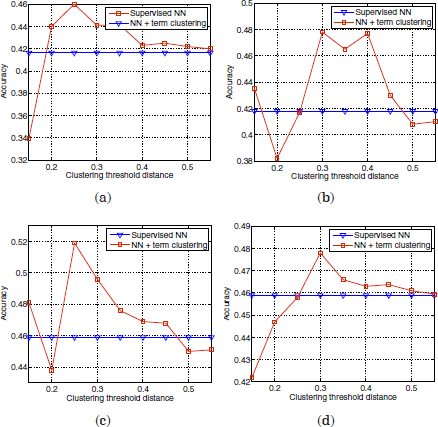
Figure 3.14 shows the mean accuracy scores obtained by the supervised algorithm versus the semi-supervised approach (before and after disambiguation) over 20 different initializations.
Standard deviations are indicated as shadowed areas around their respective mean curves. Figure 3.14a shows the classification accuracy of the supervised scheme and the semi-supervised approach with disambiguation, using the term vector definition of equation [3.11]. Figure 3.14b refers to the term vector definition in equation [3.10]. As can be observed, by incorporating the disambiguation scheme, the semi-supervised approach achieves notable improvements with respect to the supervised classifier, up to 65% accuracy.
Figure 3.14. Mean accuracy values achieved by the supervised classifier vs. the semi-supervised approach before and after disambiguation. Standard deviations are indicated as shadowed areas around their respective mean curves. (a): Supervised NN based on bag of words features vs. semi-supervised using semantic class features. (b): Supervised vs. semi-supervised by incorporating word vector truncation
3.6. Summary
In this chapter, a semi-supervised classification scheme has been described. It takes advantage of the availability of unlabeled data by means of unsupervised clustering applied to the feature space of words. This approach is based on the hypothesis that synonymy is one important source of variability in the utterances for a single symptom. Thus, by identifying clusters of semantically related terms, the vocabulary available to the classifier can be “augmented.” One of the main contributions in this work is the novel definition of a word in a vector space model so that any distance metric applied to word vectors can capture the degree of semantic dissimilarity between the words. When using a term vector model with term truncation (so that only the most important words in the context of another word wi account for the definition of the ith word vector), the semi-supervised approach has shown average accuracy improvements up to 5% with respect to the basic supervised classifier.
This has been motivated by the observation that a significant amount of ambiguities resulted from the proposed classification schemes. Ambiguities are basically due to the cooccurrences of words representative for different categories.
1. In this book, the context of a word wi is defined at the utterance level, i.e. the words that co-occur with wi in the same utterance.