
4
Optimum Receiver
We defined a signal and random process in Chapter 2 and looked into wireless channels in Chapter 3. Now, we need to know how to detect a transmitted signal correctly in a receiver. The main purpose of the receiver is to recover the transmitted signal from the distorted received signal. Decision theory is helpful for finding the original signal. Decision theories are widely used in not only wireless communication systems but also other applications. Almost everything people face in their day-to-day life is related to decisions. For example, every day, we have to decide on the color of outfit that we have to wear, what to eat, and which route to drive. For example, if we need to find a shortcut to a particular place, then we have to decide based on the following: a priori information (or a prior probability) such as weather forecast or traffic report, an occurrence (or a probability of occurrence) such as traffic jam, and a posterior information (or a posterior probability) such as data collected regarding traffic jam. Likewise, we have to decide on the messages a transmitter sends in a wireless communication system. The decision depends on a priori information such as modulation type and carrier frequency, an occurrence such as a measured signal, and a posterior information such as channel state information. The decision theory of wireless communication systems is developed to minimize the probability of error. In this chapter, several decision theories are introduced and optimum receiver is discussed.
4.1 Decision Theory
We consider a simple system model with a discrete channel as shown in Figure 4.1.

Figure 4.1 System model based on a discrete channel
The wireless channel models we discussed in Chapter 3 are analogue channel models.
In communication theory (especially, information or coding theory), a digital channel model is mainly used such as a discrete channel, Binary Symmetric Channel (BSC), Binary Erasure Channel (BEC), and so on. In this system model, the message source produces a discrete message, mi, (where i = 1, …, M) as a random variable. The probability the message, mi, appears is a priori probability, P(mi). The transmitter produces a signal, si, which are the values corresponding to the message, mi. The signal, si, becomes the input of the discrete channel. The output, rj, can be expressed as a conditional probability, P(rj|si), which means the probability that the output, rj, is received when the transmitter sends the signal, si. The receiver estimates the transmitted messages, ![]() , as the output of the receiver using the decision rule, f( ), namely
, as the output of the receiver using the decision rule, f( ), namely ![]() . The decision rule is a function mapping the received signal to the most probable value. The probability of error is defined as follows:
. The decision rule is a function mapping the received signal to the most probable value. The probability of error is defined as follows:
The receiver is designed to minimize the probability of error, Pε. The receiver minimizing the probability of error is called an optimum receiver. Let us consider a message source which can produce a random value. A transmitter sends it to a receiver over a discrete channel. In the receiver side, it would be very difficult to decide correctly if we make a decision from scratch. However, if we have a priori information, for example, the transmitted information is “0” or “1” and the probability the transmitter sends “0” is 60%, the receiver can decide correctly with 60% accuracy even if we regard all received signals as “0.” The decision theory uses a priori information, a posterior information, and likelihood. The Bayesian decision rule [1] is used when there is a priori information and likelihood. More specifically, the Bayesian formula is defined as follows:
The Bayesian decision rule with equal cost is
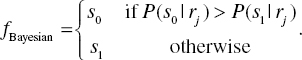
Equivalently,

The occurrence term, P(rj), is not used in the Bayesian decision rule. The probability of error is
If the likelihood is identical, the Bayesian decision rule depends on a priori information. Likewise, if the priori information is identical, it depends on the likelihood.
An optimal decision means there is no better decision which brings a better result. We define the optimal decision as maximizing ![]() as follows:
as follows:
Using the Bayesian formula,

where arg max function is defined as follows:
Therefore, the optimum receiver is designed by maximizing a posteriori probability. We call this Maximum a Posteriori (MAP) decision rule. When a priori probability, P(mi), is identical, the optimal decision can be changed as follows:
The optimum receiver relies on the likelihood. Therefore, we call this Maximum Likelihood (ML) decision rule.
4.2 Optimum Receiver for AWGN
In this section, we consider a simple system model with the AWGN channel as shown in Figure 4.3.

Figure 4.3 System model with AWGN
We consider two types of the message source outputs (mi = “0” or “1”), two types of the corresponding signals (si = s1 or s2), and s1 > s2. The probability density function of the Gaussian noise is expressed as follows:

The noise, n, is independent of the signal, s. The likelihood, ![]() depends on the probability density function of the Gaussian noise. We can express the likelihood as follows:
depends on the probability density function of the Gaussian noise. We can express the likelihood as follows:

where i = 1 or 2. The MAP decision rule as the optimal decision is expressed as follows:

We decide ![]() if the above inequalities are satisfied and
if the above inequalities are satisfied and ![]() otherwise. We derive a simple decision rule from the above equation as follows:
otherwise. We derive a simple decision rule from the above equation as follows:


Thus, we obtained (4.17) as a simple decision rule. When the priori probabilities ![]() are identical, (4.17) depends on the likelihood and becomes simpler as follows:
are identical, (4.17) depends on the likelihood and becomes simpler as follows:
When we have ![]() ,
, ![]() , and
, and ![]() , the likelihood,
, the likelihood, ![]() , can be illustrated in Figure 4.4.
, can be illustrated in Figure 4.4.

Figure 4.4 Likelihood for AWGN
The ML decision rule is that ![]() if rj is greater than 0 and
if rj is greater than 0 and ![]() otherwise. Now, we find the probability of error for the MAP decision rule. When s1 is transmitted, we decide rj > r0. Likewise, when s2 is transmitted, we decide rj ≤ r0. Thus, the probability of error is
otherwise. Now, we find the probability of error for the MAP decision rule. When s1 is transmitted, we decide rj > r0. Likewise, when s2 is transmitted, we decide rj ≤ r0. Thus, the probability of error is
The likelihood terms falling on the incorrect place can be expressed as follows:

Let

Then,

where Q(x) is called the complementary error function. It is defined as follows:

Likewise,


Therefore, we obtain the following equation from (4.19), (4.22), and (4.26):

When the priori probabilities ![]() are identical, we get
are identical, we get
and manipulate (4.28) as follows:
Therefore, the probability of error for the ML decision is

Now, we consider a continuous time waveform channel as shown in Figure 4.5 and find an optimal receiver.

Figure 4.5 System model with waveform channel
In the waveform channel, the Gaussian noise, nw(t), is generated by a random process. The autocorrelation function is expressed as follows:
and the power spectral density is
The received waveform, r(t), is expressed as follows:
where the signal, si(t), can be assembled by a linear combination of N orthonormal basis function, ϕj(t), as follows:


The orthonormal basis functions, ϕj(t), are orthonormal as follows:

The coefficients, sij, are the projection of the waveform, si(t), on the orthonormal basis and the signal set, sijϕj(t), can be represented in an N-/ this signal space [2].
Now, we discuss several operations in the signal space. The length of a vector, si, is defined as follows:

If two vectors, si and sk, are orthogonal, ![]() . For n-tuples signal space,
. For n-tuples signal space, ![]() n, the inner product of two vectors, si and sk, is defined as follows:
n, the inner product of two vectors, si and sk, is defined as follows:

The energy of the waveform, s(t), is expressed by the length of a vector as follows:


The distance from 0 to a vector, si, is ![]() . The distance between two vectors, si and sk, is
. The distance between two vectors, si and sk, is

The angle, θik, between two vectors, si and sk, is expressed as follows:

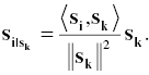
We consider the vector, si, as the sum of two vectors as follows:
where ![]() is collinear with sk and
is collinear with sk and ![]() is orthogonal to sk as shown in Figure 4.7.
is orthogonal to sk as shown in Figure 4.7.

Figure 4.7 One dimensional projection
The vector, ![]() , is called the projection of si on sk. It is expressed as follows:
, is called the projection of si on sk. It is expressed as follows:
We can now define Gram–Schmidt orthogonalization process [3] using (4.48) as follows:
The normalized vector, ei, is expressed as follows:

We call this vectors Gram–Schmidt orthonormalization.
We now discuss the received signal. The received signal is expressed as follows:
The vector representation of (4.50) is

and each element can be expressed as follows:

where j = 1, 2, …, N. (4.54) means the received signal is assembled by the orthonormal basis functions, ϕj(t). The mean and variance of the received signal is expressed as follows:
As we observed wireless channels in Chapter 3, the transmitted signals are experienced in different channels so that the received signal, r(t), can be composed of two received signals, r1(t) and r2(t), as shown in Figure 4.9.
Figure 4.9 System model with two channels
We consider the received signal and its projection on the two-dimensional signal space as shown in Figure 4.10.

Figure 4.10 Received signal and its projection on the two-dimensional signal space
The received signal, r(t) (=r1(t) + r2(t)), is composed of the transmitted signal, si(t), and the noise, nw(t). The projection of the received signal, r(t), on the two-dimensional signal space is represented as r1(t) which is composed of the transmitted signal, si(t), and the noise, n(t). Therefore, the element, r2(t), of the received signal, r(t), is irrelevant to estimate the transmitted signal, si(t) and an optimum receiver can be designed through investigating r1(t). We call this theorem of irrelevance.
4.3 Matched Filter Receiver
The optimum receiver is composed of mainly two parts. The first part is to decide the receive signal vector
where

The second part is to determine ![]() to minimize the probability of error. Namely, the decision rule
to minimize the probability of error. Namely, the decision rule

is to minimize the probability of error. In (4.59), the term, ![]() , is independent of index i
, is independent of index i ![]() . Therefore, the decision rule is to maximize the following equation:
. Therefore, the decision rule is to maximize the following equation:

An optimum correlation receiver composed of a signal detector and a signal estimator is illustrated in Figures 4.11 and 4.12.

Figure 4.11 Signal detector of an optimum correlation receiver

Figure 4.12 Signal estimator of an optimum correlation receiver
When the orthonormal basis function, ϕj(t), is zero outside a finite time interval, ![]() , we can replace a multiplier and an integrator by a matched filter and a sampler in the signal detector of an optimum correlation receiver. A matched filter and a sampler can be helpful for designing an optimum receiver easily because the accurate multiplier and integrator are not easy to implement. Consider a linear filter with an impulse response,
, we can replace a multiplier and an integrator by a matched filter and a sampler in the signal detector of an optimum correlation receiver. A matched filter and a sampler can be helpful for designing an optimum receiver easily because the accurate multiplier and integrator are not easy to implement. Consider a linear filter with an impulse response, ![]() . When r(t) is the input of the linear filter, the output of the linear filter can be described by
. When r(t) is the input of the linear filter, the output of the linear filter can be described by


When the output of the linear filter is sampled at t = T,

The impulse response of the linear filter is a delayed time-reversed version of the orthonormal basis function, ϕj(t), as shown in Figure 4.13.
Figure 4.13 (a) Orthonormal bases function, ϕj(t), and (b) the impulse response, hj(t)
We call this linear filter matched to ϕj(t). An optimum receiver with this linear filter is called a matched filter receiver. The signal detector of a matched filter receiver is illustrated in Figure 4.14.

Figure 4.14 Signal detector of a matched filter receiver
4.4 Coherent and Noncoherent Detection
The matched filter receiver can be used for the coherent detection of modulation schemes. Consider a coherent M-ary Phase Shift Keying (MPSK) system. The transmitted signal, si(t), is expressed as follows:

where ![]() ,
, ![]() , and Es is the signal energy for symbol duration T. If we assume the two-dimensional signal space, the orthonormal basis function, ϕj(t) is
, and Es is the signal energy for symbol duration T. If we assume the two-dimensional signal space, the orthonormal basis function, ϕj(t) is

Therefore, the transmitted signal, si(t), is expressed as follows:

When considering Quadrature Phase Shift Keying (QPSK), M = 4, the transmitted signal, si(t), has four signals which is expressed by a combination of two orthonormal basis function ϕ1(t) and ϕ2(t). The transmitted signal, si(t), is expressed as follows:

The transmitted signal, si(t), can be represented in the two-dimensional signal space as shown in Figure 4.15.

Figure 4.15 Two-dimensional signal space and decision regions for QPSK modulation
The two-dimensional signal space is divided into four regions. If the received signal, r(t), falls in region 1, we decide the transmitter sent s1(t). If the received signal, r(t), falls in region 2, we decide the transmitter sent s2(t). We decide s3(t) and s4(t) in the same way. The signal estimator in Figure 4.12 needs M correlators for the demodulation of MPSK. The received signal, r(t), of MPSK system is expressed as follows:

where ![]()
![]() and n(t) is white Gaussian noise. The demodulator of MPSK system can be designed in a similar way to the matched filter receiver as shown in Figure 4.16.
and n(t) is white Gaussian noise. The demodulator of MPSK system can be designed in a similar way to the matched filter receiver as shown in Figure 4.16.

Figure 4.16 Demodulator of MPSK system
The arctan calculation part is different from an optimum correlation receiver of Figure 4.12. In Figure 4.16, X is regarded as the in-phase part of the received signal, r(t), and Y is regarded as the quadrature-phase part of the received signal, r(t). The result, ![]() , of arctan calculation is compared with a prior value, θi. For QPSK modulation, it has four values (0, π/2, π, and 3 π/2 in radian) as shown in Figure 4.15. We choose the smallest phase difference as the transmitted signal,
, of arctan calculation is compared with a prior value, θi. For QPSK modulation, it has four values (0, π/2, π, and 3 π/2 in radian) as shown in Figure 4.15. We choose the smallest phase difference as the transmitted signal, ![]() .
.
Unlike the coherent detection, the noncoherent detection cannot use the matched filter receiver because the receiver does not know a reference (such as the carrier phase and the carrier frequency) of the transmitted signal. The Differential Phase Shift Keying (DPSK) system is basically classified as noncoherent detection scheme but sometime it is categorized as differentially coherent detection scheme. Consider a DPSK system. The transmitted signal, si(t), is expressed as follows:

where ![]() and
and ![]() . The received signal, r(t), is expressed as follows:
. The received signal, r(t), is expressed as follows:

where ![]()
![]() , θd is constant with a finite interval,
, θd is constant with a finite interval, ![]() , and n(t) is white Gaussian noise. If the unknown phase, θd, varies relatively slower than two symbol durations (2T), the phase difference between two consecutive received signal is independent of the unknown phase, θd as follows:
, and n(t) is white Gaussian noise. If the unknown phase, θd, varies relatively slower than two symbol durations (2T), the phase difference between two consecutive received signal is independent of the unknown phase, θd as follows:
Therefore, we can use the carrier phase of the previous received signal as a reference. The modulator of binary DPSK is illustrated in Figure 4.17.

Figure 4.17 Modulator of DPSK system
The binary message, mi, and the delayed differentially encoded bits, di−1, generates the differentially encoded bits, di, by modulo 2 addition ![]() . The differentially encoded bits, di, decide the phase shift of the transmitted signal. Table 4.1 describes an example of encoding process.
. The differentially encoded bits, di, decide the phase shift of the transmitted signal. Table 4.1 describes an example of encoding process.
Table 4.1 Example of binary DPSK encoding
| i | 0 | 1 | 2 | 3 | 4 | 5 | 6 | 7 |
| mi | 1 | 0 | 1 | 0 | 0 | 1 | 1 | |
| di−1 | 1 | 0 | 0 | 1 | 1 | 1 | 0 | |
| di | 1 | 0 | 0 | 1 | 1 | 1 | 0 | 1 |
The example of the differentially encoded bits, di, and corresponding phase shift, θi(t), is illustrated in Figure 4.18.

Figure 4.18 Example of phase shift and waveform of DPSK modulator
When we detect the differentially encoded signal, we do not need to estimate a phase of carrier. Instead, we use the phase difference between the present signal phase and the previous signal phase as shown in Figure 4.19. In the DPSK demodulator, we need the orthonormal basis function, ϕj(t), as the reference carrier frequency but do not need a prior value, θi as the reference phase.

Figure 4.19 Demodulator of DPSK system
The DPSK modulation is simple and easy to implement because we do not need to synchronize the carrier. However, the disadvantage of the DPSK modulation is that one error of the received signal can propagate to other received signals detection because their decision is highly related.
4.5 Problems
- 4.1. Consider a simple communication system as shown in Figure 4.2 and a priori probability, P(mi), and a conditional probability, P(rj|si), have the following probabilities:
mi P(mi) P(r0|si) P(r1|si) P(r2|si) 0 0.4 0.2 0.3 0.5 1 0.6 0.7 0.1 0.2 Design the decision rule with the minimum error probability.
- 4.2. Consider a simple communication system with the following system parameters:

Calculate the probability of error for MAP and ML decision.
- 4.3. Consider a signal with the following parameters:

Represent the signal, si(t), geometrically.
- 4.4. Consider a signal set, S, with the following parameters:

Find the orthogonal set, S′ = {g1, g2} using Gram–Schmidt orthogonalization process.
- 4.5. A user needs to buy a new mobile phone but it is not easy to find good mobile phone
 . Thus, the user decides to observe a gadget review website. The range of the grade is from 0 to 100. The mobile user’s estimation of the possible losses is given in the following table and the class conditional probability densities are known to be approximated by normal distribution as
  and
and  . Find the grade to minimize the risk.
α(decision, mgood) α(decision, mbad) Purchase 0 30 No purchase 5 0 - 4.6. Consider BPSK signals with
 and
and  . When the prior probabilities are
  and
and  , find the metrics for MAP and ML detector in AWGN.
 - 4.7. When we transmit the signals in successive symbol intervals, each signal is interdependent and the receiver is designed by observation of the received sequence. Design the maximum likelihood sequence detector.
- 4.8. Consider three signals:
 ,
,  , and s1(t) = cos
  . Check whether or not they are linearly independent.
 - 4.9. The digital message (0 or 1) can be encoded as a variation of the amplitude, phase, and frequency of a sinusoidal signal. For example, binary amplitude shift keying (BASK), binary phase shift keying (BPSK), and binary frequency shift keying (BFSK). Draw their waveform and express in signal space.
- 4.10. Draw the decision regions of the minimum distance receiver for 16QAM.
- 4.11. Compare the bit error probabilities for the following binary systems: coherent detection of BPSK, coherent detection of differentially encoded BPSK, noncoherent detection of orthogonal BFSK.
- 4.12. Describe the relationship between Eb/N0 and SNR.
References
- [1] E. T. Jaynes, “Bayesian Methods: General Background,” In J. H. Justice (ed.), Maximum-Entropy and Bayesian Methods in Applied Statistics, Cambridge University Press, Cambridge, pp. 1–15, 1986.
- [2] J. M. Wozencraft and I. M. Jacobs, Principles of Communication Engineering, John Wiley & Sons, Inc., New York, 1965.
- [3] G. Arfken “Gram-Schmidt Orthogonalization,” In Mathematical Methods for Physicists, Academic Press, Orlando, FL, 3rd edition, pp. 516–520, 1985.