
6
Error Correction Codes
In Part II, we design key wireless communication blocks such as error correction codes, OFDM, MIMO, channel estimation, equalization, and synchronization. The floating point design step is to check the reliability of each block in wireless communication system design flows. In this step, we select suitable algorithms and evaluate their performances. The floating point design is getting more important because the modern wireless communication system design flow is automated and many parts of the back-end design flow are already optimized. Thus, we focus on the floating point design in this book. In Part III, we will deal with the wireless communication system design flow and system integration in detail. An error correction code is an essential part of wireless communication systems. In this chapter, we design the turbo encoder/decoder, turbo product encoder/decoder, and Low-Density Parity Check (LDPC) encoder/decoder. These codes opened a new era of coding theory because their performance is close to the Shannon limit. We look into design criteria, describe the algorithms, and discuss hardware implementation issues.
6.1 Turbo Codes
6.1.1 Turbo Encoding and Decoding Algorithm
The turbo codes [Ref. 4 in Chapter 5] achieved very low error probability which is close to the Shannon limit. They became an essential part of many broadband wireless communication systems. The idea of the revolutionary error correction codes originates from concatenated encoding, randomness, and iterative decoding. The turbo encoder is composed of two Recursive Systematic Convolutional (RSC) encoders as component codes. Two component encoders are concatenated in parallel. The important design criteria of the turbo codes are to find suitable component codes which maximize the effective free distance [1] and to optimize the weight distribution of the codewords at a low EbN0 [2]. A random interleaver is placed between two component encoders. The information (or message) bits are encoded by one component encoder and reordered by a random interleaver. The permuted information bits are encoded by another component encoder. Then, we can puncture parity bits to adjust the code rate. The weight distribution of the turbo codes is related to how the codeword from one component encoder correlates the codeword from another component encoder. The random interleaver plays an important role as preventing codeword paring between two component encoders and makes codewords from each component encoder statistically independent. A random interleaver design is not easy because there is no standardized method. However, the important design criteria of a random interleaver are to find a low complexity implementation and produce both low-weight codewords from one component encoder and high-weight codewords from another component encoder simultaneously. One example of the turbo encoder structure with code rate 1/3 is illustrated in Figure 6.1.

Figure 6.1 Turbo encoder
As we can observe from Figure 6.1, the turbo encoder is systematic because the information sequence m is same as coded bit c0. Each RSC encoder includes two shift registers (memories). Thus, a finite state machine represents the state as the content of the memory. The output of each RSC encoder is calculated by modulo-2 addition among the input bit and the stored bits in two shift registers. The memory states and the outputs corresponding to the inputs are summarized in Table 6.1. We can transform this table into a state diagram or a trellis diagram as we did in Chapter 5. The trellis diagram is widely used to represent turbo encoding process. Thus, we express this table as the trellis diagram as shown in Figure 6.2.
Table 6.1 Memory states (M1 M2), inputs, and outputs of RSC encoder
| Time | Input (mi) | Memory state (M1 M2) | Output |
| 0 | 00 | ||
| 1 | 1 | 10 | 11 |
| 2 | 1 | 01 | 10 |
| 3 | 0 | 10 | 00 |
| 4 | 0 | 11 | 01 |
| 5 | 1 | 11 | 10 |
| 6 | 0 | 01 | 01 |
| 7 | 1 | 00 | 11 |
| 8 | 0 | 00 | 00 |

Figure 6.2 Trellis diagram of RSC encoder
The turbo decoder based on an iterative scheme is composed of two Soft Input Soft Output (SISO) component decoders. Figure 6.3 illustrates the turbo decoder structure.

Figure 6.3 Turbo decoder
As we can observe from Figure 6.3, two component decoders give and take their output as a priori information and reduce the error probability of the original information bits. The SISO decoder is based on the Maximum a Posteriori (MAP) algorithm (also known as Bahl-Cocke-Jelinek-Raviv (BCJR) algorithm). The RSC encoders 1 and 2 of the turbo encoder correspond to the SISO decoders 1 and 2 of the turbo decoder, respectively. The turbo decoder receives three inputs (r0, r1, and r2). The SISO decoder 1 uses the information sequence (r0), the parity sequence (r1) by RSC encoder 1, and a priori (or extrinsic) information. The SISO decoder 2 uses the interleaved information sequence (r0), the parity sequence (r2) by RSC encoder 2, and a priori information. The SISO decoder 1 starts decoding without a priori information at first and provides the SISO decoder 2 with the output as a priori information. The SISO decoder 2 starts decoding with this priori information, interleaved information r0, and parity r2. In the iteration process, the SISO decoder 1 receives a priori information from the SISO decoder 2 and decodes with a priori information, information r0, and parity r1 again. This iteration enables the decoder to reduce the error probability of the information bits but brings a long latency. In addition, the coding gain decreases rapidly at the high number of iteration.
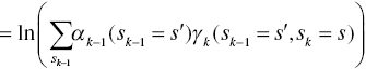
Due to the high complexity, long latency, and high energy consumption of the MAP algorithm, it was not widely used until the turbo codes appear. Both the MAP algorithm and the Viterbi algorithm have similar decoding performance but the Viterbi algorithm does not produce soft outputs. Thus, the Viterbi algorithm is not suitable for the component decoder of the turbo decoder. The MAP decoder formulates the bit probabilities as soft outputs using the Log Likelihood Ratio (LLR). The soft output of the first MAP decoder is defined as follows:
The LLR calculates and compares the probabilities when the information mk is +1 and −1 after observing two inputs ![]() . We calculate the probability when the information mk is +1 using the Bayes’ theorem as follows:
. We calculate the probability when the information mk is +1 using the Bayes’ theorem as follows:


Likewise, we calculate the probability when the information mk is −1 as follows:


Now, we reformulate the LLR in terms of the trellis diagram as follows:

where sk denotes the state at time k in the trellis diagram, s′ and s are a state of the trellis diagram, and Sp and Sn are transition sets of the trellis diagram when ![]() and
and ![]() , respectively. Figure 6.4 illustrates the transition set of Figure 6.2 trellis diagram.
, respectively. Figure 6.4 illustrates the transition set of Figure 6.2 trellis diagram.

Figure 6.4 Transition sets of Figure 6.2 trellis diagram
The numerator and denominator probability term of the LLR can be rewritten as follows:
Then, we define the forward path metric ![]() , the backward path metric
, the backward path metric ![]() , and the branch metric
, and the branch metric ![]() as follows:
as follows:
Thus, (6.9) is rewritten as follows:

and (6.8) is rewritten using the above three metrics as follows:

The forward path metric is calculated from time index k−1 to time index k as follows:
The initial value of the forward path metric is given as follows:

because the RSC encoder starts at state 0 (00 in the example). The backward path metric is calculated from time index k + 1 to time index k as follows:
Likewise, the initial value of the backward path metric is given as follows:

because we generally terminate the trellis at state 0 (00 in the example). The branch metric is rewritten as follows:
where ![]() and
and ![]() represent a likelihood probability and a priori probability, respectively. The likelihood probability is expressed as follows:
represent a likelihood probability and a priori probability, respectively. The likelihood probability is expressed as follows:

where ω0 and ω1 are very small values and these terms are ignored. The priori probability is expressed as follows:

where

The branch metric is rewritten as follows:
where
Now, we reformulate LLR as follows:


where ![]() and
and ![]() do not depend on state transition. Thus, (6.41) is written as follows:
do not depend on state transition. Thus, (6.41) is written as follows:
where ![]() is the initial priori information of the MAP algorithm,
is the initial priori information of the MAP algorithm, ![]() is the channel value, and
is the channel value, and ![]() is the extrinsic information. The extrinsic information is used as a priori information of the second MAP decoder.
is the extrinsic information. The extrinsic information is used as a priori information of the second MAP decoder.
6.1.2 Example of Turbo Encoding and Decoding
Consider the turbo encoder with code rate 1/3 as shown in Figure 6.1 and the trellis diagram of the RSC encoder as shown in Figure 6.2. When the input sequence is [1 1 0 0 1], the initial state (T0) of the memory is “00,” and the two tailing bits are [0 1], we can express the input, output, and memory state in the trellis diagram as shown in Figure 6.5. As we can observe from Figure 6.5, there is the unique path in the trellis diagram of the RSC encoder 1.

Figure 6.5 Encoding example of RSC encoder 1
Figure 6.5 shows that the output of the RSC encoder 1 is [11 10 00 01 10 01 11]. We define the random interleaver of the turbo encoder as shown in Figure 6.6.

Figure 6.6 Random interleaver of the turbo encoder
After the information sequence is passed through the random interleaver, the input of the RSC encoder 2 becomes [0 1 1 0 1 1 0]. Likewise, we have the unique path in the trellis diagram of the RSC encoder 2 as shown in Figure 6.7.

Figure 6.7 Encoding example of RSC encoder 2
The output of the RSC encoder 2 is [00 11 10 00 10 11 00]. Thus, the output of the turbo encoder is c0 = [c10, c20, c30, c40, c50, c60, c70] = [1 1 0 0 1 0 1], c1 = [c11, c21, c31, c41, c51, c61, c71] = [1 0 0 1 0 1 1], and c2 = [c12, c22, c32, c42, c52, c62, c72] = [0 1 0 0 0 1 0].
We map the output into the symbol of BPSK modulation and transmit it sequentially. Thus, the transmitted symbol sequence is [c10, c11, c12, c20, c21, c22, … , c70, c71, c72] → [+1 +1 −1 +1 −1 +1 −1 −1 −1 −1 +1 −1 +1 −1 −1 −1 +1 +1 +1 +1 −1]. In the channel, the transmitted symbol sequence is added by Gaussian noise as shown in Figure 6.8. In the receiver, the turbo decoder as shown in Figure 6.3 uses the received symbol sequence [r0 r1 r2] as the soft decision input. The first MAP decoder (SISO decoder 1) of the turbo decoder starts decoding. As we observed the above MAP algorithm, it is much more complex than the Viterbi algorithm. Thus, we simplify the MAP algorithm with a view to reducing implementation complexity. The Log-MAP algorithm and the Max-log-MAP algorithm as suboptimal algorithms provide us with a reasonable complexity. The Log-MAP algorithm is based on the following approximation:

Figure 6.8 Channel noise example
The Max-log-MAP algorithm is based on the following approximation:
According to Ref. [3], The Max-log-MAP algorithm has less complexity than the Log-MAP algorithm but brings about 0.35 dB performance degradation in the turbo decoding. Besides these approximations, the Soft Output Viterbi Algorithm (SOVA) which is modified by the Viterbi algorithm enables the decoder to emit soft decision outputs. Its complexity is decreased by about half of the MAP algorithm. However, the performance drop is about 0.6 dB. In this section, we describe the Max-log-MAP algorithm. The forward path metric is simplified as follows:
and the initial value of the forward path metric is given as follows:

The backward path metric is simplified as follows:


and the initial value of the backward path metric is given as follows:

The branch metric is simplified as follows:

where we assume
Thus, we obtain the simplified branch metric as follows:
Using these simplified metrics and the trellis diagram, we firstly calculate the branch metrics of the first MAP decoder as follows:
Figure 6.9 illustrates the branch metric calculations of the first MAP decoder on the trellis diagram.

Figure 6.9 Branch metric calculations of the first MAP decoder
From (6.49), the forward path metrics are calculated as follows:
Figure 6.10 illustrates the forward path metric calculations of the first MAP decoder on the trellis diagram.

Figure 6.10 Forward path metric calculations of the first MAP decoder
From (6.54), the backward path metrics are calculated as follows:
Figure 6.11 illustrates the backward path metric calculations of the first MAP decoder on the trellis diagram.

Figure 6.11 Backward path metric calculations of the first MAP decoder
If the packet length is long, the forward and backward path metric values grow constantly and overflow in the end. Thus, we generally normalize the forward and backward path metrics at each time slot because the difference between the path metrics is important. There are two ways to normalize path metrics. The first approach is to subtract a specific value from each metric. The specific value can be selected by the average or the largest path metric of the other path metrics in each time slot. Besides, we can divide the path metrics by the sum of them in each time slot. This approach is simple but not efficient to implement hardware because the additional calculation is needed and it increases the latency. The other approach is to let overflow happen and observe them. For example, we divide the path metric memory into three parts (low, middle, and high). In a specific time slot, one path metric is in high part and the other path metric is in low part. We select the path metric in high part.
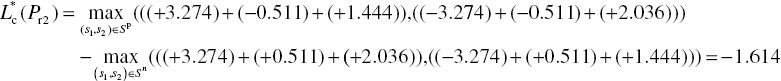
Finally, we simplify (6.39) using the Max-log-MAP algorithm and have the following LLR:

Thus, we calculate the soft decision outputs of the first MAP decoder as follows:
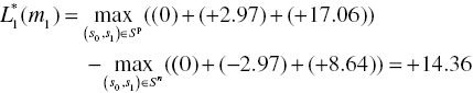


From (6.43), we express the extrinsic information for the second MAP decoder as follows:
and it is calculated as shown in Table 6.2.
Table 6.2 Extrinsic information for the second MAP decoder in the first iteration
| k | ||||
| 1 | +10.12 | +14.36 | 0 | 2·(+2.12) |
| 2 | +9.9 | +13.64 | 0 | 2·(+1.87) |
| 3 | −8.52 | −11.8 | 0 | 2·(−1.64) |
| 4 | −12.42 | −11.8 | 0 | 2·(+0.31) |
| 5 | +8.02 | +11.8 | 0 | 2·(+1.89) |
| 6 | −9.46 | −13.04 | 0 | 2·(−1.79) |
| 7 | +11.62 | +12 | 0 | 2·(+0.19) |
The extrinsic information ![]() is used for a priori information of the second MAP decoder after interleaving. It becomes the input of the second MAP decoder together with the interleaved information r0 and the parity r2 from the RSC encoder 2. Thus, we have the following inputs:
is used for a priori information of the second MAP decoder after interleaving. It becomes the input of the second MAP decoder together with the interleaved information r0 and the parity r2 from the RSC encoder 2. Thus, we have the following inputs: ![]() , r0 = [+0.31 +1.89 +1.87 −1.64 +0.19 +2.12 −1.79] and r2 = [−2.27 +1.71 −0.62 −1.77 −1.33 +1.92 −1.74]. In the same way as the first MAP decoding, we start decoding. Firstly, the second MAP decoders are calculated as follows:
, r0 = [+0.31 +1.89 +1.87 −1.64 +0.19 +2.12 −1.79] and r2 = [−2.27 +1.71 −0.62 −1.77 −1.33 +1.92 −1.74]. In the same way as the first MAP decoding, we start decoding. Firstly, the second MAP decoders are calculated as follows:
Figure 6.12 illustrates the branch metric calculations of the second MAP decoder on the trellis diagram.

Figure 6.12 Branch metric calculations of the second MAP decoder
From (6.49), the forward path metrics are calculated as follows:
Figure 6.13 illustrates the forward path metric calculations of the first MAP decoder on the trellis diagram.
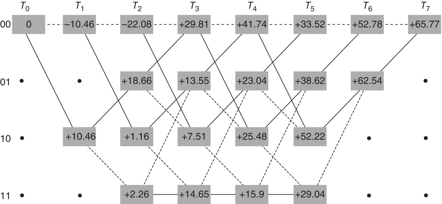
Figure 6.13 Forward path metric calculations of the second MAP decoder
From (6.54), the backward path metrics are calculated as follows:
Figure 6.14 illustrates the backward path metric calculations of the first MAP decoder on the trellis.

Figure 6.14 Backward path metric calculations of the second MAP decoder
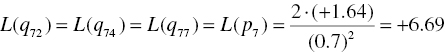
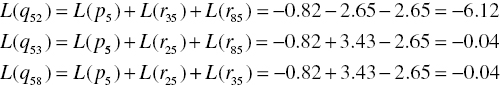
Finally, we calculate the soft decision outputs of the second MAP decoder as follows:


Thus, the output of the second MAP decoder is [−7.6 +23.68 +23.68 −7.6 +35.68 +33.42 −16.22]. After de-interleaving, we can obtain [+33.42 +23.68 −7.6 −7.6 +23.68 −16.22 +35.68] and calculate the extrinsic information for the first MAP decoder in the second iteration as shown in Table 6.3.
Table 6.3 Extrinsic information for the first MAP decoder in the second iteration
| k | ||||
| 1 | +19.06 | +33.42 | +10.12 | 2·(+2.12) |
| 2 | +10.04 | +23.68 | +9.9 | 2·(+1.87) |
| 3 | +4.2 | −7.6 | −8.52 | 2·(−1.64) |
| 4 | +4.2 | −7.6 | −12.42 | 2·(+0.31) |
| 5 | +11.88 | +23.68 | +8.02 | 2·(+1.89) |
| 6 | −3.18 | −16.22 | −9.46 | 2·(−1.79) |
| 7 | +23.68 | +35.68 | +11.62 | 2·(+0.19) |
This extrinsic information ![]() is used for the priori information of the first MAP decoder in the second iteration. The iteration can continue. Basically, the error correction capability increases while the iteration continues. It will converge to a stable value around six or seven iterations. In this example, we obtained [+1 +1 −1 −1 +1 −1 +1] as the output of the turbo decoder after hard decision. Now, we can observe that we received the corrupted fourth bit but it was fixed by the turbo decoder.
is used for the priori information of the first MAP decoder in the second iteration. The iteration can continue. Basically, the error correction capability increases while the iteration continues. It will converge to a stable value around six or seven iterations. In this example, we obtained [+1 +1 −1 −1 +1 −1 +1] as the output of the turbo decoder after hard decision. Now, we can observe that we received the corrupted fourth bit but it was fixed by the turbo decoder.
6.1.3 Hardware Implementation of Turbo Encoding and Decoding
In the previous sections, we derived the turbo encoder and decoder algorithm and understood their encoding and decoding process. Now, we look into hardware implementation issues of the turbo encoder and decoder. There are several key design requirements such as power, complexity, throughput, and latency. When dealing with a mobile application, the low power is highly required and power consumption becomes a key design parameter. When dealing with a high-speed communication system, the throughput and the latency become key design parameters. The complexity is directly related to design cost and system performance. It is always a key parameter we should carefully consider. Thus, we firstly look into a simple hardware implementation of the turbo encoder and decoder in this section. Then, we estimate the design parameters and identify the target design goal.
The hardware architecture of the turbo encoder is same as the conceptual diagram in Figure 6.1. As we can observe Figure 6.1, the turbo encoder is composed of shift registers and modulo 2 adders. It can be easily implemented. The random interleaver of the turbo encoder can be implemented by a look-up table. However, the disadvantage of a look-up table is high latency. Thus, several standards such as 3GPP [4] or 3GPP2 [5] use a simple digital logic to implement it. A hardware architecture of the MAP decoder as a SISO decoder includes four main blocks as shown in Figure 6.15.

Figure 6.15 MAP decoder architecture
As we investigated in Sections 6.1.1 and 6.1.2, the MAP decoder receives the soft decision input and firstly calculates branch metrics indicating the Euclidean distances. As we discussed in Chapter 5, the soft decision input can be expressed as the 2b−1 level where b is the bit resolution. This bit level significantly affects the complexity of the MAP decoder. It becomes a basis of each metric calculation. Basically, we should carefully choose the bit level because a higher bit level brings a higher performance and complexity. The optimal quantization width (T) depends on a noise level as shown in Figure 6.16. It can be calculated as follows:

where N0 is a noise power spectral density. The four or three bits soft decision input is widely used because it is good trade-off between performance and complexity. The branch metric block can be simply implemented by addition and multiplication.

Figure 6.16 Quantization width
Secondly, we calculate the forward and backward path metric selecting one path in the trellis diagram. As we can observe the trellis diagram in Figure 6.2, the trellis diagram at each stage has symmetry characteristic. We call this symmetry a butterfly structure. Two states are paired in a butterfly structure as shown in Figure 6.17. The butterfly structure is useful for simplifying the forward and backward path metric calculation.
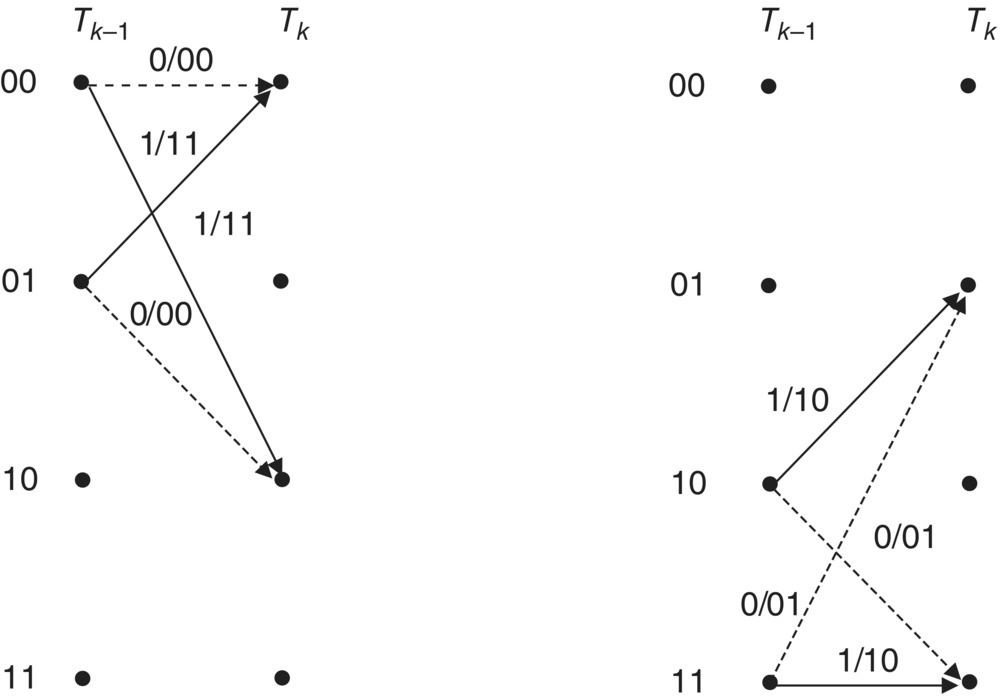
Figure 6.17 Butterfly structure of Figure 6.2 trellis diagram
These are based on the Add-Compare-Select (ACS) block as shown in Figure 6.18. The ACS block in the figure is designed for the Log-MAP algorithm. In the figure, the dashed lines and blocks represent the calculation of the term “![]() .”
.”

Figure 6.18 Add-Compare-Select block
The term of log calculation (or correction function) is not easy to implement in a digital logic. It has a high complexity. Figure 6.19 illustrates the correction function. Thus, it can be implemented by a Look-Up Table. If we remove the dashed lines and blocks, it is the ACS block of the Max-log-MAP algorithm. In the forward and backward path metric calculation block, the normalization block should be employed to prevent an overflow as mentioned in Section 6.1.2. Subtractive normalization can be implemented by subtraction and average.

Figure 6.19 Correction function
Thirdly, we design the LLR block using addition, subtraction, and compare. In order to calculate the LLR, we need all branch metrics and forward and backward path metrics. It requires very large memory to hold them. Thus, the sliding window technique [6] is widely used to minimize the memory size. The sliding widow technique defines a window size (L) which is independent of the initial condition. In the window, the forward and backward path metric can be calculated. The calculation result in the window is almost same as the calculation result in the whole frame. Most importantly, it reduces the latency because it enables us to calculate them in parallel. Figure 6.20 illustrates the timing of the forward and backward calculation using the sliding window technique. In the figure, the dashed line of the backward calculation represents initialization due to unreliable branch metric calculation. For 16 states trellis diagram, the window size (L) is 32. It is approximately 6K where K is the constraint length of a convolutional encoder. The required memory is 192L bits when six-bits path metrics are used. It is not greater than the requirement of the conventional Viterbi decoder storage. The output of the LLR calculation can be used for the output of the MAP decoder or produce the extrinsic information.

Figure 6.20 Timing of the sliding window technique
Now, we estimate the design parameters. If we design the algorithm blocks using a Hardware Description Language and look into a Register-Transfer Level in a specific target hardware environment, we can obtain more accurate estimations of complexity and power consumption. However, we deal with a floating point level design in this chapter. Thus, we estimate them with simple calculation. The power and complexity depend on control signals, memories, and data path calculations (branch metrics, forward path metrics and backward path metrics, and LLRs). When designing a complex system, control signal management is one of tricky parts. Thus, a separate block such as a complex finite state machine, a firmware, or an operating system is required for control signal management. However, the MAP decoder does not require complex data paths or timing. A simple finite state machine using a counter is enough. It controls the data path and memory. In order to estimate the number of memories, we should hold information bits (Bi), parity bits (Bp), LLRs (BLLR), and path metrics (Bpm). The simple calculation about memory requirement of the MAP decoder is as follows:
where Ns and M are the number of states in the trellis diagram and the number of parallel flows, respectively. The turbo decoder needs two MAP decoders and requires double memories. In addition, a memory for a random interleaver should be considered. The complexity calculation of data paths is approximately estimated when we have the Lframe frame length and 2 Ns branches of the trellis diagram. The complexity calculations are summarized in Table 6.4. The complexity basically increases according to the number of iterations.
Table 6.4 Complexity of the Log-MAP algorithm
| Sub-blocks of the Log-MAP decoder | Complexity |
| Branch metric | 2 Ns Lframe (addition) |
| 2 Ns ·3·Lframe (multiplication) | |
| Forward path metric | 2 Ns Lframe (addition) |
| Ns Lframe (Mux) | |
| Ns Lframe (subtraction) | |
| Backward path metric | 2 Ns Lframe (addition) |
| Ns Lframe (Mux) | |
| Ns Lframe (subtraction) | |
| LLR | 2·2 Ns Lframe (addition) |
| 2·Lframe (Mux) | |
| Lframe (subtraction) |
The latency of the turbo decoder depends on the delay of the MAP decoder, the number of iteration, and the random interleaver. The delay of the MAP decoder depends on the window size, the number of parallelization, and the frame length. The number of iteration is an important part affecting the turbo decoder latency. Sometimes the number of iteration can be limited if the bit error rate (BER) performance reaches a specific value. We can observe performance saturation after six or seven iterations. The interleaver needs a whole frame to start interleaving. Thus, this is one of key latency parts. Several techniques such as parallel interleaver design or combinational logic design are developed.
6.2 Turbo Product Codes
6.2.1 Turbo Product Encoding and Decoding Algorithm
In 1954, P. Elias [7] suggested the construction of simple and powerful linear block codes from simpler linear block codes. We call them product codes. The product code is constructed using a block of information bits (I). Each row of information bits is encoded by a row component code and row parity bits (Pr) are appended to the same row. After finishing row encoding, each column of information bits is encoded by a column component code and column parity bits (Pc and Prc) are appended to the same column. The encoding process is illustrated in Figure 6.21.

Figure 6.21 Product code
Let us consider two systematic linear block codes: C1 (n1, k1, d1) and C2 (n2, k2, d2), where n, k, and d are the code length, the information (or message) length, and the minimum distance, respectively. A product code CP (n1 × n2, k1 × k2, d1 × d2) is obtained from C1 and C2. As we can observe from Figure 6.21, one information bit is encoded by both a row code and a column code. When one bit is corrupted in a receiver and cannot be corrected by a row code, a column code may fix it and vice versa. We can expand the two-dimensional product codes to m-dimensional product codes where m is larger than 2. An m-dimensional product code CPm ![]() is constructed by the m component codes (n1, k1, d1), (n2, k2, d2), …, (nm, km, dm). The component codes can be single parity check codes, Hamming codes, Reed-Muller codes, BCH codes, Reed-Solomon codes, and so on. It is also possible to use a nonlinear block code such as Nordstrom-Robinson code, Preparata codes, and Kerdock codes. R. Pyndiah in 1994 [8] introduced the turbo product codes (or block turbo codes) and presented a new iterative decoding algorithm for decoding product codes based on the Chase algorithm [9]. The turbo product encoding process is same as the product encoding process. The turbo product decoding process is an iterative decoding process based on SISO decoding algorithms such as the Chase algorithm, the symbol by symbol MAP algorithm [10], the SOVA [11], the sliding-window MAP algorithm [12], or the forward recursion only MAP algorithm [13]. The row blocks of the turbo product codes are decoded first and then all of column blocks are decoded. Iteration can be done several times to reduce the error probability. The complexity of SISO algorithms is a very important implementation issue because there is a tradeoff between complexity and performance as we discussed in Section 6.1. When comparing turbo product codes with turbo codes, the turbo product codes have two advantages. The first advantage is that the turbo product codes provide us with a better performance at a high code rate (more than 0.75). The second advantage is that the turbo product codes require smaller frame size. The turbo product decoding process is similar to the turbo code decoding process. The component decoder of the turbo product decoder is illustrated in Figure 6.22. Firstly, each SISO decoder calculates the soft output LLRi from the channel received information Ri. The extrinsic information Ei is obtained from Ri and LLRi by
is constructed by the m component codes (n1, k1, d1), (n2, k2, d2), …, (nm, km, dm). The component codes can be single parity check codes, Hamming codes, Reed-Muller codes, BCH codes, Reed-Solomon codes, and so on. It is also possible to use a nonlinear block code such as Nordstrom-Robinson code, Preparata codes, and Kerdock codes. R. Pyndiah in 1994 [8] introduced the turbo product codes (or block turbo codes) and presented a new iterative decoding algorithm for decoding product codes based on the Chase algorithm [9]. The turbo product encoding process is same as the product encoding process. The turbo product decoding process is an iterative decoding process based on SISO decoding algorithms such as the Chase algorithm, the symbol by symbol MAP algorithm [10], the SOVA [11], the sliding-window MAP algorithm [12], or the forward recursion only MAP algorithm [13]. The row blocks of the turbo product codes are decoded first and then all of column blocks are decoded. Iteration can be done several times to reduce the error probability. The complexity of SISO algorithms is a very important implementation issue because there is a tradeoff between complexity and performance as we discussed in Section 6.1. When comparing turbo product codes with turbo codes, the turbo product codes have two advantages. The first advantage is that the turbo product codes provide us with a better performance at a high code rate (more than 0.75). The second advantage is that the turbo product codes require smaller frame size. The turbo product decoding process is similar to the turbo code decoding process. The component decoder of the turbo product decoder is illustrated in Figure 6.22. Firstly, each SISO decoder calculates the soft output LLRi from the channel received information Ri. The extrinsic information Ei is obtained from Ri and LLRi by ![]() where
where ![]() is a weighting factor.
is a weighting factor.

Figure 6.22 Component decoder of the turbo product decoder
The SISO decoder is used as the row and column component decoder of the turbo product decoder. The optimal MAP or Log-MAP algorithm has high complexity. Its suboptimal variants such as the Log-MAP algorithm and the Max-log-MAP algorithm are used in practice. The SOVA is another desirable candidate because of its low complexity. However, the SOVA has poorer performance than the Max-log-MAP algorithm.
6.2.2 Example of Turbo Product Encoding and Decoding
Consider a turbo product encoder using a (4, 3, 2) Single Parity Check (SPC) code as a row and column encoder. It is defined as follows:
where ![]() , Ii, and P denote a modulo 2 adder, an information bit, and a parity bit, respectively. Thus, we obtain a (16, 9, 4) turbo product code. As shown in Figure 6.21, the encoded bits of the turbo product encoder are generated. We transmit the sequence [I11, I12, I13, Pr1, I21, I22, I23, Pr2, I31, I32, I33, Pr3, Pc1, Pc2, Pc3, Prc]. Figure 6.23 illustrates the turbo product encoding process.
, Ii, and P denote a modulo 2 adder, an information bit, and a parity bit, respectively. Thus, we obtain a (16, 9, 4) turbo product code. As shown in Figure 6.21, the encoded bits of the turbo product encoder are generated. We transmit the sequence [I11, I12, I13, Pr1, I21, I22, I23, Pr2, I31, I32, I33, Pr3, Pc1, Pc2, Pc3, Prc]. Figure 6.23 illustrates the turbo product encoding process.

Figure 6.23 Turbo product encoder
It is possible to represent the trellis of block codes. The important advantage is that the trellis representation of block codes enables us to perform MAP or ML decoding. The disadvantage is that the complexity increases when the codeword length increases. Thus, the trellis representation of block codes is suitable for short length codes such as row or column codes of the product codes. The trellis diagram of the (4, 3, 2) SPC code is shown in Figure 6.24.
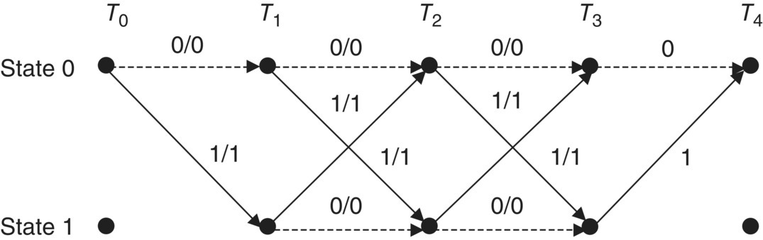
Figure 6.24 Trellis diagram of the (4, 3, 2) SPC code
In Figure 6.24, the information bits are represented from T0 to T3 and the parity bit is decided at T4. Based on this trellis diagram, the turbo product decoder can receive soft decision inputs and MAP decoding is possible. Figure 6.25 illustrates the transmitted symbols, Gaussian noise, and the received symbols.

Figure 6.25 Channel noise example
In the receiver, the turbo product decoder uses the soft decision received symbol sequence as shown in Figure 6.25. Figure 6.26 illustrates the turbo product decoder architecture.

Figure 6.26 Turbo product decoder
We perform MAP decoding for the row codes and then for the column codes. The branch metrics are calculated as follows:
For the first row decoder,
For the second row decoder,
For the third row decoder,
Figure 6.27 illustrates the branch metric calculations of the row MAP decoders.

Figure 6.27 Branch metric calculations of the first (a), second (b), and third (c) row MAP decoder
According to (6.49), the forward path metrics are calculated as follows:
For the first row decoder,
For the second row decoder,
For the third row decoder,
Figure 6.28 illustrates the forward path metric calculations of the row MAP decoders.

Figure 6.28 Forward path metric calculations of the first (a), second (b), and third (c) row MAP decoder
According to (6.54), the backward path metrics can be calculated as follows:
For the first row decoder,
For the second row decoder,
For the third row decoder,
Figure 6.29 illustrates the backward path metric calculations of the row MAP decoders.

Figure 6.29 Backward path metric calculations of the first (a), second (b), and third (c) row MAP decoder
From branch, forward path, and backward path metrics, we calculate the soft decision output of the row MAP decoder as follows:
For the first row decoder,


For the second row decoder,


For the third row decoder,


Finally, we obtain the row decoding results in the first iteration as shown in Figure 6.30.

Figure 6.30 Row decoding results in the first iteration
We had three corrupted bits (I22, I31, and I33) in the received symbol sequence. I22 is fixed after the row decoding but I31 and I33 are not fixed. The output of the row decoder is multiplied by ![]() which is the weighting factor to adjust the effect of the LLR value. The extrinsic information Ei can be obtained by subtracting the soft input of the MAP decoder from the soft output of the MAP decoder as follows:
which is the weighting factor to adjust the effect of the LLR value. The extrinsic information Ei can be obtained by subtracting the soft input of the MAP decoder from the soft output of the MAP decoder as follows:
The input of the column decoder is obtained by adding the received sequence R with the extrinsic information Ei as follows:
where ![]() is the weighting factor to adjust the extrinsic information. The experimental results indicate that the performance of the turbo product decoder is very sensitive to the weighting factors [14]. We define
is the weighting factor to adjust the extrinsic information. The experimental results indicate that the performance of the turbo product decoder is very sensitive to the weighting factors [14]. We define ![]() and
and ![]() in this example. Thus, we obtain the column decoder inputs in the first iteration as shown in Figure 6.31.
in this example. Thus, we obtain the column decoder inputs in the first iteration as shown in Figure 6.31.

Figure 6.31 Column decoder inputs in the first iteration
The column decoder can be implemented in the same manner as the row MAP decoder. The branch metrics for the column decoder are calculated as follows:
For the first column decoder,
For the second column decoder,
For the third column decoder,
For the fourth column decoder,
Figure 6.32 illustrates the branch metric calculations of the column MAP decoders.

Figure 6.32 Branch metric calculations of the first (a), second (b), third (c), and fourth (d) column MAP decoder
According to (6.49), the forward path metrics are calculated as follows:
For the first column decoder,
For the second column decoder,
For the third column decoder,
For the fourth column decoder,
Figure 6.33 illustrates the forward path metric calculations of the column MAP decoders.

Figure 6.33 Forward path metric calculations of the first (a), second (b), third (c), and fourth (d) column MAP decoder
According to (6.54), the backward path metrics are calculated as follows:
For the first column decoder,
For the second column decoder,
For the third column decoder,
For the fourth column decoder,
Figure 6.34 illustrates the backward path metric calculations of the column MAP decoders.

Figure 6.34 Backward path metric calculations of the first (a), second (b), third (c), and fourth (d) column MAP decoder
From branch, forward path, and backward path metrics, we calculate the soft decision outputs of the column MAP decoder as follows:
For the first column decoder,


For the second column decoder,


For the third column decoder,


For the fourth column decoder,

Finally, we obtain the column decoding results in the first iteration as shown in Figure 6.35.

Figure 6.35 Column decoding results in the first iteration
As we can observe in Figure 6.35, I31 and I33 were not fixed after the row decoding. However, they are fixed in the column decoder. In the same way, the second iteration is performed or the output of the turbo product decoder is determined by hard decision.
6.2.3 Hardware Implementation of Turbo Product Encoding and Decoding
As we investigated in Section 6.2.1, turbo product codes are constructed by systematic block codes. The encoding process of the turbo product codes can be easily implemented by shift registers and modulo 2 adders. The encoding complexity is proportional to the codeword length. Figure 6.36 illustrates an example of a (4, 3, 2) single parity check encoder and a (7, 4) Hamming encoder.

Figure 6.36 Example of a (4, 3, 2) SPC encoder (a) and a (7, 4, 3) Hamming encoder (b)
The turbo product decoder is composed of row and column component decoders. Unlike turbo codes, the turbo product codes do not need an interleaver and each component code is independent. Thus, it is easy to build a parallel architecture. If we design a (n, k, d)2 turbo product code with same component codes (N row codes and N column codes), the turbo product decoder can have simple parallel decoding architecture as shown in Figure 6.37.

Figure 6.37 Parallel turbo product decoder
In the first iteration, the first memory (M1) holds the received codeword and sends each row codeword to component decoders. The second memory (M2) holds the results of each row decoder and sends extrinsic information to the first memory after scaling it. In the second iteration, the first memory sends the received codeword and extrinsic information as a priori information. Each component decoder performs column decoding. Figure 6.38 illustrates the component decoder.

Figure 6.38 Component decoder of the turbo product decoder
Since we used the Max-log-MAP algorithm as component decoders of the turbo product decoder, the turbo product decoding process is same as the turbo decoding process. The parallel turbo product decoder enables us to implement a high speed decoding. However, the memory size and the complexity increase. In order to reduce them, we can design a serial turbo product decoder which uses a single component decoder. Since each row and column code can be decoded by a single component, we can approximately reduce the memory size and complexity by a factor of N even if the latency increases.
6.3 Low-Density Parity Check Codes
6.3.1 LDPC Encoding and Decoding Algorithms
In 1962, R. Gallager [Ref. 1 in Chapter 5] originally invented LDPC codes during his PhD. However, the LDPC codes were not widely recognized until D.J.C Mackay and R.M. Neal [Ref. 2 in Chapter 5] rediscovered them as the era of transistors has just started and the hardware technology did not cover the complexity of LDPC encoding and decoding at that time. After the turbo codes emerged in 1993, many researchers have made an effort to prove theoretically how the turbo codes achieve near Shannon limit and have tried to find another new error correction code. In 1996, Mackay and Neal designed a new linear block code including many similar features of turbo codes such as randomness, large block length, and iterative decoding. They soon realized that the new codes are almost same as LDPC codes by Gallager. After that, irregular LDPC codes as generalization of Gallager’s LDPC codes are developed by Luby et al. [15] in 1998. The irregular LDPC codes became the most powerful error control codes as of now. When comparing with the turbo codes, LDPC codes have several advantages. Firstly a random interleaver is not required. Secondly, it has a better block error rate and a lower error floor. Thirdly, iterative decoding of LDPC codes is simple even if it requires more iterations. The most highlighted advantage is that it is patent-free.
As the name implies, LDPC codes are linear block codes with a sparse parity check matrix H. The sparseness of the parity check matrix H means that H contains relatively few 1s among many 0s. The sparseness enables LDPC codes to increase the minimum distance. Typically, the minimum distance of LDPC codes linearly increases according to the codeword length. Basically, LDPC codes are same as conventional linear block codes except the sparseness. The difference between LDPC codes and conventional linear block codes is decoding method. The decoder of the conventional linear block codes is generally based on ML decoding which receives n bits codeword and decides the most likely k bits message among the 2k possible messages. Thus, the codeword length is short and the decoding complexity is low. On the other hands, LDPC codes are iteratively decoded using a graphical representation (Tanner graph) of H. The Tanner graph is consisted of bit (or variable, symbol) nodes and check (or parity check) nodes. The bit nodes and the check nodes represent codeword bits and parity equations, respectively. The edge represents a connection between bit nodes and check nodes if and only if the bit is involved in the corresponding parity check equation. Thus, the number of edges in a Tanner graph means the number of 1s in the parity check matrix H. Figure 6.39 illustrates an example of a Tanner graph. The squares represent check nodes (or parity check equations) and the circles represent bit nodes in the figure.
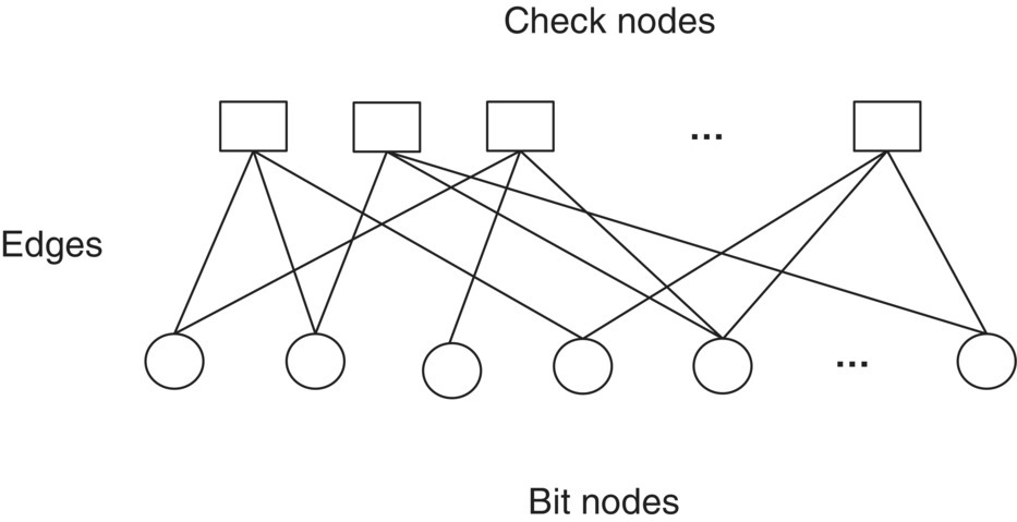
Figure 6.39 Example of Tanner graph
As we observed in Chapter 5, a linear block code has a (n−k) × n parity check matrix H. The rows and columns of H represent the parity check equations and the coded bits, respectively.
The regular LDPC code by Gallager is denoted as (n, bc, br) where n is a codeword length, bc is the number of parity check equations (or 1s per column), and br is the number of coded bits (or 1s per row). The regular LDPC code has the following properties: (i) each coded bit is contained in the same number of parity check equations and (ii) each parity check equation contains the same number of coded bits. The regular LDPC code by Gallager is constructed by randomly choosing the locations of 1s with the fixed numbers in each row and column. The rows of the parity check matrix are divided into bc sets. Each set has n/br rows. The first set contains r consecutive 1s descending from left to right. The other sets are obtained by column permutation of the first set.
Another LDPC code construction by Mackay and Neal fills 1s in the parity check matrix H from left column to right column. The locations of 1s are randomly chosen in each column until each row with the fixed numbers is assigned. If some row is already filled, the row is not assigned and the remaining rows are filled. One important constraint is that the 1s in each column and row should not be square shape. It is important to avoid a cycle of length 4. However, it is not easy to satisfy this constraint. The number of br and bc should be small when comparing with the code length.
In a Tanner graph, a cycle is defined as a node connection starting and ending at same node. The length of the cycle is defined as the number of edges of the cycle. The cycle prevents performance improvement of iterative decoding because it affects the independence of extrinsic information during the iterative process. Thus, it is important to remove cycles in the parity check matrix. Sometimes a cycle breaking technique can be used to remove cycles as shown in Figure 6.41. This technique changes the Tanner graph and can reduce the number of cycles. However, it increases the number of nodes so that the complexity of iterative decoding increases.

Figure 6.41 Cycle breaking (column splitting (a) and row splitting (b))
The girth of a Tanner graph is defined as the length of the shortest cycle in the Tanner graph. The shortest cycle in a Tanner graph is 4. In the Example 6.3, the girth is 6. The short cycles disturb performance improvement during iterative process of decoding algorithms. Thus, it is one important parameter to maximize the girth when designing a LDPC encoder.

Figure 6.42 Cycle of length 4 and the related edges between the bit nodes (c4 and c7) and the check nodes (Eq1 and Eq2)
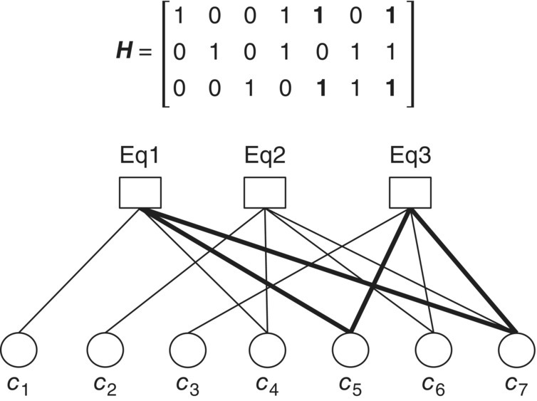
Figure 6.43 Cycle of length 4 and the related edges between the bit nodes (c5 and c7) and the check nodes (Eq1 and Eq3)

Figure 6.44 Cycle of length 4 and the related edges between the bit nodes (c6 and c7) and the check nodes (Eq2 and Eq3)

Figure 6.45 Cycle of length 6 and the related edges between the bit nodes (c4, c5 and c6) and the check nodes (Eq1, Eq2 and Eq3)
Irregular LDPC codes are generalization of regular LDPC codes. In the parity check matrix of irregular LDPC codes, the degrees of bit nodes and check nodes are not constant. Thus, an irregular LDPC code is represented as degree distribution of bit nodes and check nodes. The bit node degree distribution is defined as follows:

where Λi and db are the number of bit nodes of degree i and the maximum bit nodes, respectively. The check node degree distribution is defined as follows:

where Pi and dc are the number of check nodes of degree i and the maximum check nodes, respectively. It is possible to represent in the edge point of view. The bit node degree distribution in the edge point of view is defined as follows:

where λi is the fraction of edges connected to bit nodes of degree i. The check node degree distribution in the edge point of view is defined as follows:

where ρi is the fraction of edges connected to check nodes of degree i. The design rate of an LDPC code is bounded by

It is not easy to optimize an irregular LDPC code design. Many approaches to construct an irregular LDPC code are based on computer search. As we discussed in Chapter 5, the generator matrix of a linear block code can be obtained from the parity check matrix. Using Gauss–Jordan elimination, we change the form of the party check matrix H as follows:
where P and In−k are a parity matrix and an identity matrix, respectively. Thus, the generator matrix is
The sparseness of P determines the complexity of LDPC encoders. Unfortunately, P is most likely not spare even if the constructed H is sparse. Basically, a LDPC code requires a long frame size (a large n). The encoding complexity is O(n2) so that the encoding complexity is one important design issue. There are many approaches to reduce encoding complexity [16].
The decoding process of LDPC codes is based on the iteration scheme between bit nodes and check nodes in a Tanner graph. A decoding scheme of LDPC codes is known as a message passing algorithm which passes messages forward and backward between the bit nodes and check nodes. There are two types of message passing algorithms: the bit flipping algorithm based on a hard decision decoding algorithm and the belief propagation algorithm based on a soft decision decoding algorithm. The belief propagation algorithm calculates the maximum a posteriori probability (APP). That is to say, it calculates the probability ![]() , which means we find a codeword ci on the event E (all parity check equations are satisfied). In the belief propagation algorithm, the message represents the belief level (probability) of the received codewords. Each bit node passes a message to each check node connected to the bit node. Each check node passes a message to each bit node connected to the check node. In the final stage, APP of each codeword bit is calculated. We should calculate many multiplication and division operations for the belief propagation algorithm. Thus, the implementation complexity is high. In order to reduce the complexity, it is possible to implement it using log likelihood ratios. Multiplication and division are replaced by addition and subtractions, respectively. We call this a sum-product decoding algorithm. In order to explain the belief propagation algorithm, the Tanner graph is modified. Figure 6.46 illustrates an example of the Tanner graph for LDPC decoding.
, which means we find a codeword ci on the event E (all parity check equations are satisfied). In the belief propagation algorithm, the message represents the belief level (probability) of the received codewords. Each bit node passes a message to each check node connected to the bit node. Each check node passes a message to each bit node connected to the check node. In the final stage, APP of each codeword bit is calculated. We should calculate many multiplication and division operations for the belief propagation algorithm. Thus, the implementation complexity is high. In order to reduce the complexity, it is possible to implement it using log likelihood ratios. Multiplication and division are replaced by addition and subtractions, respectively. We call this a sum-product decoding algorithm. In order to explain the belief propagation algorithm, the Tanner graph is modified. Figure 6.46 illustrates an example of the Tanner graph for LDPC decoding.

Figure 6.46 Tanner graph example for LDPC decoding
In Figure 6.46, vj, xi, and yi represent check nodes, bit nodes, and received codeword bits, respectively. We express the received codeword as follows:
where ni is Gaussian noise with zero mean and standard deviation σ. We define two messages (estimations): qij(x) and rji(x). The message qij(x) and the message rji(x) represent the message from the bit node xi to the check node vj and the message from the check node vj to the bit node xi, respectively. They can be expressed in the Tanner graph as shown in Figure 6.47.

Figure 6.47 Two messages in the Tanner graph
The message qij(x) means the probability ![]() or the probability xi = x satisfying all check node equations except vj. The message rji(x) means the probability the parity check node (parity check equation) vj is satisfied when all bit nodes have x except xi. Thus, message passing can be described as shown in Figure 6.48.
or the probability xi = x satisfying all check node equations except vj. The message rji(x) means the probability the parity check node (parity check equation) vj is satisfied when all bit nodes have x except xi. Thus, message passing can be described as shown in Figure 6.48.

Figure 6.48 Example of bit node (a) and check node (b) message passing in the Tanner graph
In the AWGN channel, we have the following initial value of qijinitial(x):

where x = +1 or −1 (assume BPSK modulation). When the received vector y with the length L is given, Gallager described the probability that the parity check nodes contain an even or odd number of 1s is expressed as follows:

where

and pi is ![]() which is the probability that the codeword bit at i is equal to −1. Thus, the message rji(+1) is expressed as follows:
which is the probability that the codeword bit at i is equal to −1. Thus, the message rji(+1) is expressed as follows:

where Vj/i denotes a bit node set connected to the check node vj except xi. We express ![]() as follows:
as follows:
The message ![]() is expressed as follows:
is expressed as follows:
and the message ![]() is expressed as follows:
is expressed as follows:
where Ci/j denotes a check node set connected to the bit node xi except vj and the constant αij are selected to ensure that ![]() . In this way, we start calculating rji(x) using the initial values of qij(x). The message qij(x) is calculated by rji(x). Then, we calculate the APP ratio for each codeword bit as follows:
. In this way, we start calculating rji(x) using the initial values of qij(x). The message qij(x) is calculated by rji(x). Then, we calculate the APP ratio for each codeword bit as follows:
where the constant αij are selected to ensure that ![]() . Lastly, the hard decision outputs are calculated as follows:
. Lastly, the hard decision outputs are calculated as follows:

The iteration process is continued until the estimated codeword bits satisfy the syndrome condition or the maximum number of iteration is finished.
Due to the high complexity of the belief propagation algorithm, a sum-product algorithm in the log domain is more suitable for hardware implementation. The initial value of qij(x) as log likelihood ratio is expressed as follows:


The message rji(x) as log likelihood ratio is expressed as follows:

Using the relationship

we reformulate (6.88) as follows:

because


However, (6.90) still has multiplication. We need to further reformulate as follows:


where

and

Now, L(rji) does not include multiplication but the complexity is still high. The function f(x) is not simple function as shown in Figure 6.49. It can be implemented by a look-up table.

Figure 6.49 Function f(x)
Thus, further simplification using a min-sum algorithm is possible as follows:

because the minimum term of ![]() dominates in the equation. The performance degradation caused by further approximation is about 0.5 dB. However, if a scaling factor (α) [17] is added as follows:
dominates in the equation. The performance degradation caused by further approximation is about 0.5 dB. However, if a scaling factor (α) [17] is added as follows:

the performance degradation can be reduced to 0.1 dB. The message qij(x) as log likelihood ratio is expressed as follows:


Then, we calculate the log APP ratio for each codeword bit as follows:
Lastly, the hard decision outputs are calculated as follows:

Similar to the belief propagation algorithm, the iteration continues until the syndrome condition is satisfied or the maximum number of iterations is reached.
6.3.2 Example of LDPC Encoding and Decoding
We construct an irregular LDPC code having the following parity check matrix H:
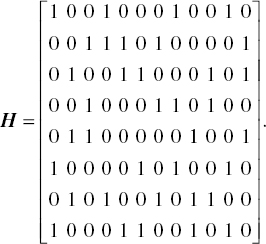
The Tanner graph of the parity check matrix H is drawn as shown in Figure 6.50.

Figure 6.50 Tanner graph of (6.104)
Using Gauss–Jordan elimination, we change the form of (6.104) as follows:

From (6.105), we find the generator matrix of the irregular LDPC code as follows:

The message m = [1 0 1 0] generates the codeword [1 1 0 1 0 1 1 1 1 0 1 0] by mG. The codeword is modulated by BPSK modulation. The modulated symbol sequence [+1 +1 −1 +1 −1 +1 +1 +1 +1 −1 +1 −1] is transmitted. After passing through AWGN channel with the standard deviation σ = 0.7 as shown in Figure 6.51, the LDPC decoder receives the symbol [+1.11 +1.20 −1.44 +0.84 −0.20 −0.65 +1.64 +1.15 +0.95 −1.22 +1.13 −0.98]. We can observe that an error occurs at the sixth codeword symbol.

Figure 6.51 Channel noise example
We use a sum-product algorithm in the log domain. The initialization of L(qij) is carried out as the first step of the LDPC decoding as follows:


The second step is to calculate L(rji) from check nodes to bit nodes. L(r11) is calculated by the initial values of the L(q41), L(q81), and L(q111) as follows:

Figure 6.52 illustrates the calculation process of L(r11).

Figure 6.52 Calculations of L(r11)
In the same way, we calculate the remaining L(rji) as follows:


The third step is to calculate L(qij) from bit nodes to check nodes. L(q11) is calculated by L(p1), L(r61), and L(r81) as follows:
Figure 6.53 illustrates the calculation process of L(q11).

Figure 6.53 Calculations of L(q11)
In the same way, we calculate the remaining L(qij) as follows:


The fourth step is to calculate L(Qi) as follows:
After the hard decision of the APPs, we obtain [+1 +1 −1 +1 −1 +1 +1 +1 +1 −1 +1 −1]. Thus, the estimated codeword bits ![]() are [1 1 0 1 0 1 1 1 1 0 1 0]. The syndrome test is carried out as follows:
are [1 1 0 1 0 1 1 1 1 0 1 0]. The syndrome test is carried out as follows:

Since the syndrome result is all zero, the LDPC decoder stops iteration and estimates [1 1 0 1 0 1 1 1 1 0 1 0] is the transmitted codeword. Thus, the decoded message ![]() is [1 0 1 0]. If the syndrome result is not all zero, the iteration continues until the syndrome result is all zero or the maximum number of iteration is reached.
is [1 0 1 0]. If the syndrome result is not all zero, the iteration continues until the syndrome result is all zero or the maximum number of iteration is reached.
6.3.3 Hardware Implementation of LDPC Encoding and Decoding
As we discussed in the previous section and Chapter 5, a codeword of a LPDC code can be constructed by performing c = mG. The generator matrix G (=[Ik P] or [P Ik]) is created by a parity check matrix H. We should make the parity check matrix in a systematic form H (=[PT In−k] or [In−k PT]) using Gauss–Jordan elimination. However, it is very difficult to have a sparse P matrix. A codeword construction by c = mG is not simple. Especially, the complexity of a LDPC code construction is one critical problem in a large codeword length. Thus, many researchers developed a low complexity LDPC encoding. In [18], two steps encoding method with the low complexity (0.0172n2+O(n)) is developed. As the first step is called preprocessing, the parity check matrix is rearranged into several submatrices as follows:

where A, B, T, C, D, and E are of size (m−g) × (n−m), (m−g) × g, (m−g) × (m−g), g × (n−m), g × g, and g × (m−g), respectively. T is a lower triangular sub-matrix with 1s along the diagonal. All sub-matrices are spares because the parity check matrix is rearranged by only row and column permutations. Figure 6.54 illustrates the rearranged parity check matrix in approximate lower triangular form.

Figure 6.54 Rearranged parity check matrix
In the lower triangular form, a gap g should be as small as possible. The sub-matrix E is cleared by performing the pre-multiplication as follows:

We check whether or not ![]() is singular. If it is singular, the singularity should be removed. The second step is to construct codeword c = (u, p1, p2) where u is an information part and p1 (length g) and p2 (length m−g) are parity parts. Since HcT = 0, we have the following equations:
is singular. If it is singular, the singularity should be removed. The second step is to construct codeword c = (u, p1, p2) where u is an information part and p1 (length g) and p2 (length m−g) are parity parts. Since HcT = 0, we have the following equations:

From (6.111), we obtain the first parity part p1 as follows:
where ![]() . In the same way, we obtain the second parity part p2 from (6.110) as follows:
. In the same way, we obtain the second parity part p2 from (6.110) as follows:
Another easy encoding of LDPC codes is to use cyclic or quasi cyclic code characteristics. A Quasi Cyclic (QC) LDPC code [19] has sub-matrices with cyclic or quasi cyclic characteristics. It can be constructed by shifting sub-matrices.
In the LDPC decoder, there are many design issues such as complexity, power consumption, latency, interconnection between nodes, scheduling, error floor reduction, reconfigurable design for multiple code rates and codeword lengths. According to interconnection between nodes, LDPC decoder architectures can be classified into fully parallel LDPC decoders, partially parallel LDPC decoders, and serial LDPC decoders. In the fully parallel LDPC decoder, each node of the Tanner graph is directly mapped into a processing unit as shown in Figure 6.55. The number of Check processing Node Units (CNUs) and Bit processing Node Units (BNUs) is same as the number of rows and columns, respectively. The number of interconnections is same as the number of edges. Each CNU and BNU calculates the probability (or logarithms of probabilities) and passes a message to opposite nodes through interconnections. The fully parallel LDPC decoder architecture provides us with the highest throughput. We don’t need scheduling and a large size memory. However, it requires the maximum number of calculations and interconnections. For a large codeword, the interconnection is very complex and difficult to implement. Another disadvantage is that it is not flexible. CNU, BNU, and interconnection are fixed. It could not support multiple code rates and codeword lengths. The complexity of the fully parallel LDPC decoder is proportional to the codeword length.

Figure 6.55 Fully parallel LDPC decoder architecture
The partially parallel LDPC decoder architecture as shown in Figure 6.56 provides us with a lower complexity and a better scalability than the fully parallel LDPC decoder. The number of CNUs, BNUs, and interconnections in the partially parallel LDPC decoder is much smaller than them in the fully parallel LDPC decoder because they are shared. The grouping of CNUs and BNUs can be carried out according to cycles. The interconnection and scheduling of messages depend on the grouping. However, the partially parallel LDPC decoder has a lower throughput and needs scheduling. The throughput is proportional to the number of CNUs and BNUs. Thus, the number of CNUs and BNUs should be selected in terms of the required throughput.

Figure 6.56 Partially parallel LDPC decoder architecture
The serial LDPC decoder architecture as shown in Figure 6.57 has only one CNU and BNU. Thus, it provides us with the minimum hardware complexity. The CNU and BNU calculate one row and column at a time. In addition, it is highly scalable and can satisfy any code rates or codeword lengths. However, the throughput is extremely low. Thus, it is difficult to apply a practical system because the most of wireless communication system require a high throughput.

Figure 6.57 Serial LDPC decoder architecture
The latency of a LDPC decoder is one of the disadvantages. Typically, LPDC codes need about 25 iterations to converge but turbo codes converge the performance in about 6 or 7 iterations. The latency is related to node calculations, interconnections, and scheduling. In order to reduce the node calculation, approximations such as the min-sum algorithm can be used. Most of the low complexity algorithms [20] have a near optimum performance. The quantization level of the input signal in a LDPC decoder is one of the important design parameters. This is highly related to decoding performance, memory size, and complexity. They are a trade-off between decoding performance and complexity. About four to six bits level brings a good balance between them [21, 22]. Another disadvantage of LDPC decoder is that it is not easy to design reconfigurable decoders because it naturally has a random structure. Thus, a new class of LDPC codes such as QC-LDPC and structured LDPC code [23] are widely used in many wireless communication systems. The QC-LDPC code structure composed of square sub-matrices allows us to efficiently design the partially parallel LDPC decoder.
6.4 Problems
- 6.1. Consider the (2, 1, 1) RSC code with generator matrix G(D) = [1 1/(1 + D)]. Draw the trellis diagram.
- 6.2. Consider the turbo encoder composed of two RSC codes of Problem 6.1 and a random interleaver. Describe the turbo encoding and decoding process when the code rate is 1/2 (Puncturing) and 1/3 (no puncturing).
- 6.3. Find the minimum free distance of the turbo code in Problem 6.2.
- 6.4. In one of 3GPPP standards, the turbo code is defined as follows:
- Code rate = 1/2, 1/3, 1/4, and 1/5
- The transfer function of the component code is
G(D) = [1 n0(D)/d(D) n1(D)/d(D)]
where d(D) = 1 + D2 + D3, n0(D) = 1 + D + D3 and n1(D) = 1 + D + D2 + D3. - Puncturing patterns
| Output | Code rate | |||
| 1/2 | 1/3 | 1/4 | 1/5 | |
| X | 11 | 11 | 11 | 11 |
| Y0 | 10 | 11 | 11 | 11 |
| Y1 | 00 | 00 | 10 | 11 |
| X′ | 00 | 00 | 00 | 00 |
| 01 | 11 | 01 | 11 | |
| 00 | 00 | 11 | 11 | |
-
- Random interleaver
Design the turbo encoder and decoder.
- Random interleaver
- 6.5. Consider the turbo product encoder composed of two (7, 4, 3) Hamming codes as row and column encoder. Design the turbo product decoder using Chase algorithm.
- 6.6. Explain why turbo product codes have a lower error floor than turbo codes.
- 6.7. Consider the following parity check matrix

6.8. Find the parity check equations and draw the corresponding Tanner graph.
- 6.9. Construct the parity check matrix of a (20, 3, 4) regular LDPC code by (i) Gallager and (ii) Mackay and Neal.
- 6.10. Find the cyclic of the parity check matrix in Problem 6.8 and perform cycle breaking.
- 6.11. Extrinsic Information Transfer (EXIT) charts provide us with a graphical depiction of density evolution. Draw the EXIT chart for (20, 3, 4) regular LDPC code in Problem 6.8.
- 6.12. Describe the encoding and decoding process of a (20, 3, 4) regular LDPC code.
References
- [1] D. Divslar and R. J. McEliece, “Effective Free Distance of Turbo Codes,” Electronic Letters, vol. 32, no. 5, pp. 445–446, 1996.
- [2] D. Divsalar and F. Pollara, “One the Design of Turbo Codes,” TDA Progress Report 42-123, Jet Propulsion Lab, Pasadena, CA, pp. 99–121, 1995.
- [3] P. Robertson, P. Hoeher, and E. Villebrun, “Optimal and Sub-optimal Maximum a Posteriori Algorithms Suitable for Turbo Decoding,” European Transactions on Telecommunications, vol. 8, pp. 119–125, 1997.
- [4] 3rd Generation Partnership Project (3GPP), Technical Specification Group Radio Access Network, “Multiplexing and Channel Coding (FDD),” W-CDMA 3GPP TS 25.212 v6.3, December 2004.
- [5] CDMA2000 3GPP2 C.S0002-C Version 2.0, “Physical Layer Standard for cdma200 Spread Spectrum Systems” July 23, 2004.
- [6] A. J. Viterbi, “An Intuitive Justification and a Simplified Implementation of the MAP Decoder for Convolutional Codes,” IEEE Journal on Selected Areas in Communications, vol. 16, no. 2, pp. 260–264, 1998.
- [7] P. Elias, “Error-Free Coding,” IRE Transactions on Information Theory, vol. PGIT-4, pp. 29–37, 1954.
- [8] R. Pyndiah, A. Glavieux, A. Picart, and S. Jacq, “Near Optimum Decoding of Product Codes,” IEEE Global Telecommunications Conference (GLOBECOM’94), San Francisco, CA, vol. 1, pp. 339–343, November 28, 1994.
- [9] D. Chase, “A Class of Algorithms for Decoding Block Codes with Channel Measurement Information,” IEEE Transactions on Information Theory, vol. IT-18, pp. 170–182, 1972.
- [10] L. R. Bahl, J. Cocke, F. Jelinek, and J. Raviv, “Optimal Decoding of Linear Codes for Minimizing Symbol Error Rate,” IEEE Transactions on Information Theory, vol. IT-20, pp. 284–297, 1974.
- [11] J. Hagenauer and P. Hoeher, “A Viterbi Algorithm with Soft-Decision Output and its Applications,” IEEE Global Telecommunications Conference (GLOBECOM’89), Dallas, TX, vol. 3, pp. 1680–1686, November 27–30, 1989.
- [12] S. S. Pietrobon and S. A. Barbulescu, “A Simplification of the Modified Bahl Algorithm for Systematic Convolutional Codes,” Proceedings of IEEE International Symposium on Information Theory and Its Applications (ISITA’94), pp. 1071–1077, Sydney, Australia, November 20–25, 1994.
- [13] Y. Li, B. Vucetic, and Y. Sato, “Optimum Soft-Output Detection for Channels with Intersymbol Interference,” IEEE Transactions on Information Theory, vol. 41, no. 3, pp. 704–713, 1995.
- [14] H. Kim, G. Markarian, and V. Rocha, “Low Complexity Iterative Decoding of Product Codes Using a Generalized Array Code Form of the Nordstrom-Robinson Code,” Proceedings of the 6th International Symposium on Turbo Codes and Iterative Information Processing, pp. 88–92, Brest, France, September 6–10, 2010.
- [15] M. G. Luby, M. Mitzenmacher, M. A. Shokrollahi, and D. A. Speilman, “Improved Low-Density Parity Check Codes Using Irregular Graphs and Belief Propagation,” Proceedings of IEEE International Symposium on Information Theory (ISIT’98), pp. 16–21, Cambridge, MA, USA, August 16–21, 1998.
- [16] T. Richardson and R. Urbanke, “Efficient Encoding of Low-Density Parity Check Codes,” IEEE Transactions on Information Theory, vol. 47, pp. 638–656, 2011.
- [17] J. Heo, “Analysis of Scaling Soft Information on Low Density Parity Check Code,” IEE Electronics Letters, vol. 39, no. 2, pp. 219–220, 2003.
- [18] T. J. Richardson and R. L. Urbanke, “Efficient Encoding of Low-Density Parity-Check Codes,” IEEE Transactions on Information Theory, vol. 47, no. 2, pp. 638–656, 2001.
- [19] M. Fossorier, “Quasi-Cyclic Low-Density Parity-Check Codes from Circulant Permutation Matrices,” IEEE Transactions on Information Theory, vol. 50, no. 8, pp. 1788–1793, 2004.
- [20] E. Elefthriou, T. Mittelholzer, and A. Dholakia, “Reduced Complexity Decoding Algorithm for Low-Density Parity Check Codes,” IEE Electronics Letter, vol.37, no. 2, pp. 102–103, 2011.
- [21] L. Ping and W. K. Leung, “Decoding Low Density Parity Check Codes with Finite Quantization Bits,” IEEE Communications Letters, vol. 4, no. 2, pp. 62–64, 2000.
- [22] Z. Zhang, L. Dolecek, M. Wainwright, V. Anantharam, and B. Nikolic, “Quantization Effects in Low-Density Parity-Check Decoder,” Proceedings of IEEE International Conference on Communications (ICC’07), pp. 6231–6237, Glasgow, UK, June 28, 2007.
- [23] R. M. Tanner, D. Sridhara, T. E. Fuja, and D. J. Costello, “LDPC Block and Convolutional Codes Based on Circulant Matrices,” IEEE Transactions on Information Theory, vol. 50, no. 12, pp. 2966–2984, 2004.