
7
Orthogonal Frequency-Division Multiplexing
The Orthogonal Frequency-Division Multiplexing (OFDM) became the most popular transmission technique for a broadband communication system because it has many advantages such as robustness to multipath fading channels and high spectral efficiency. The Orthogonal Frequency-Division Multiple Access (OFDMA) is used for a multiuser system based on the OFDM technique. It allows multiple users to receive information at the same time on different parts of the channels. The OFDMA typically allocates multiple subcarriers to an individual user. Many recent standards use the OFDM/OFDMA technique. For example, European Telecommunications Standards Institute (ETSI) included the OFDM technique in the Digital Video Broadcasting-Terrestrial (DVB-T) system in 1997. The WiFi included the OFDM technique for its physical lаyer in 1999. In addition, IEEE802.16e/m and LTE adopted the OFDMA technology. In this chapter, we design the OFDM system and discuss hardware implementation issues.
7.1 OFDM System Design
We should consider many design parameters of the OFDM system. The first design parameters of the OFDM system for wireless communications are Inter-Carrier Interference (ICI) power, the size of the Discrete Fourier Transform (DFT), and the subcarrier spacing (or the OFDM symbol duration). It is important to determine the optimal DFT size balancing protection against multipath fading, the Doppler shift, and complexity [1]. The DFT size and subcarrier spacing are related to the performance and complexity of the OFDM system. For example, when 20 MHz bandwidth is given to design an OFDM system, we can consider two designs: one OFDM system can have 64 subcarriers and 312.5 kHz subcarrier spacing and another OFDM system can have 2048 subcarriers and 15 kHz subcarrier spacing. The OFDM symbol duration is the inverse of the subcarrier spacing. Thus, their OFDM symbol durations are 3.2 µs (=1/312.5 kHz) and 66.7 µs (=1/15 kHz). Generally speaking, the short OFDM symbol duration and wide subcarrier spacing is suitable when the channel is rapidly varying in time domain and slowly varying in frequency domain. Thus, this OFDM system configuration is suitable for short-range communications. On the other hand, the long OFDM symbol duration and narrow subcarrier spacing is suitable when the channel is slowly varying in time domain and rapidly varying in frequency domain. Thus, this OFDM system configuration is suitable for cellular systems. In order to find suitable OFDM parameters, two main elements (the Doppler spread (coherence time) and multipath delay (coherence bandwidth)) should be considered. As we discussed in Chapter 3, Ts < Tc and Bs < Bc should be satisfied so that OFDM symbols experience slow and flat fading. For example, a mobile station speed 100 km/h (=28 m/s) is considered in this analysis for mobility support. This maximum speed basically provides us with good coverage of vehicular speed. The maximum Doppler shift (fm) corresponding to the operation at 3.5 GHz (wavelength = 0.086 m = 3 × 10⁸ m/s/3.5 × 109/s) is given as follows:

where ν and λ are velocity and wavelength, respectively. The symbol duration affects the ICI by the Doppler spread. The ICI degrades the OFDM system performance. A longer symbol duration basically means a higher ICI in wireless channels. In Ref. [2], a simple upper bound on the ICI power is defined as follows:
Figure 7.1 illustrates the relationship between the ICI power and fmTs.

Figure 7.1 Upper bound on the ICI power
The symbol duration Ts should be carefully selected to satisfy the condition that fmTs is small enough. Thus, the Doppler effect to the symbol must be negligible. When considering 10 kHz subcarrier spacing, the ICI power corresponding to the Doppler shift is calculated as follows:

This ICI power is less than a noise level. Thus, we can ignore the ICI power. The coherence time Tc of the wireless channel corresponding to the Doppler shift is calculated from (3.24) as follows:

This means the update rate of 770 Hz (=1/1.3 ms) is required for channel estimation and equalization. The International Telecommunications Union—Radio communication Sector Vehicular Channel Model B (ITU-VB channel model) [3, 4] shows us the rms delay spread values of up to 20 µs for mobile environments. The subcarrier spacing design requires that each subcarrier experiences flat fading for the worst-case delay spread values of 20 µs with a guard time overhead of no more than 10% for a target delay spread of 10 µs. The coherence bandwidth (Bc) of the wireless channel for correlation greater than 0.5 corresponding to the 20 µs delay spread (τrms) is calculated from (3.17) as follows:

This means that multipath fading for the delay spread values of up to 20 µs is considered to be flat fading over 10 kHz subcarrier width. The above analysis based on the coherence time, the Doppler shift, and the coherence bandwidth of the channel is the basis for the consideration of the OFDM system design. For example, when a standard defines 10 MHz bandwidth at 3.5 GHz carrier frequency and the OFDM system should support a mobile user with speed 100 km/h, the subcarrier spacing should be chosen as less than 10 kHz.
The second design parameter is the guard interval and the cyclic prefix (CP). The guard interval is used to overcome the Inter-Symbol Interference (ISI) among OFDM symbols. It should be selected as a larger interval than the maximum delay. If the maximum delay exceeds the guard interval, the signal constellation is seriously distorted. In Ref. [5], the guard interval is chosen as at least fourfold rms delay spread. The OFDM symbol duration should be much larger than the guard interval in order to prevent the SNR loss by the guard interval. However, a larger OFDM symbol duration affects the DFT size, phase noise, frequency offset, and Peak-to-Average Ratio (PAPR). Thus, the OFDM symbol duration is practically defined as at least fivefold or sixfold guard interval. For example, the rms delay spread is 100 ns. The guard interval is 400 ns (=100 ns × 4) and the OFDM symbol duration is 2.4 µs (=400 ns × 6). A cyclic prefix is used for eliminating the ISI. The guard interval consists of null signals but the cyclic prefix is composed of the OFDM symbol extension cyclically. The CP length should be larger than the channel impulse response. Thus, all distributed energy caused by multipath delay is recovered and the orthogonality is maintained. In LTE standard, two CP lengths are defined. The normal CP is used in urban (small) cells and high data rates and the extended CP is used in rural (large) cells and low data rates. The normal CP and the extended CP are defined as about 7.5 and 25% of the OFDM symbol duration, respectively. For example, the OFDM symbol duration is 2 µs. The normal CP is 150 ns and the extended CP is 500 ns. The CP is a copy of the last subcarriers in the OFDM symbol and appended at the guard interval in front of the OFDM symbol. Figure 7.2 illustrates the effect of the guard interval and cyclic prefix in the OFDM symbol. Figure 7.2a and b shows us signal distortion when there is no guard interval. Figure 7.2c and d represents that the guard interval (or Zero padding) prevents signal distortion. Figure 7.2e and f shows us overcoming multipath delay due to the CP.

Figure 7.2 Guard interval and cyclic prefix effect: No guard interval (a) and (b), guard interval (c) and (d), and guard interval with cyclic prefix (e) and (f)
The third design parameter is the pilot subcarrier allocation. The pilot signals are used for channel estimation and frequency offset/phase noise compensation. In an OFDM symbol, some subcarriers are allocated for pilots. For example, when we consider 256 DFT size of the OFDM system, 56 subcarriers are used for guard bands. Among 56 subcarriers, a low frequency guard band, a high frequency guard band, and a Direct Current (DC) signal are 28 subcarriers, 27 subcarriers, and 1 subcarrier, respectively. They are null signals. Among the remaining 200 subcarriers, data signals are 192 subcarriers and pilots are 8 subcarriers. The goal of pilot design is to find an optimum pilot allocation balancing between the spectral efficiency and the channel estimation performance. As we discussed the pilot spacing in frequency and time domain in Chapter 5, pilot spacing in frequency domain is related to the maximum delay spread (τmax). It should be smaller than the variation of the channel in frequency domain ![]() . If pilot spacing is larger than this condition, the channel cannot be accurately estimated. A wireless channel is varying during OFDM transmission. The channel variation in time domain should be estimated. The maximum pilot spacing in time domain is described by the Doppler spread and the OFDM symbol duration. It is expressed as
. If pilot spacing is larger than this condition, the channel cannot be accurately estimated. A wireless channel is varying during OFDM transmission. The channel variation in time domain should be estimated. The maximum pilot spacing in time domain is described by the Doppler spread and the OFDM symbol duration. It is expressed as ![]() (5.67). In a practical system, double sampling is often used to estimate the channel more accurately [6]. Thus, (5.67) and (5.68) are modified as follows:
(5.67). In a practical system, double sampling is often used to estimate the channel more accurately [6]. Thus, (5.67) and (5.68) are modified as follows:

and

However, there is trade-off relationship between the accuracy of the channel estimation and the spectral efficiency. Thus, pilot spacing should be designed according to system requirements. For example, we assume the maximum delay spread, the Doppler spread and the subcarrier spacing are 20 µs, 326 Hz, and 10 kHz, respectively. Using (5.67) and (5.68), we calculate the sampling interval of pilot spacing in frequency domain and the maximum pilot spacing in time domain as follows:

and
The first calculation means that the channel frequency response estimation of an OFDM system is sampled with 2.5 subcarrier spacing. Namely, the pilot symbols are needed for every two data subcarriers. If we assume L tap channel model, the DFT size (N) is equal to fpL. The second calculation means that the pilot symbol should be inserted at least every 15 OFDM symbols in order to track the channel variation. To sum up, a block-type pilot structure is suitable for this system. An optimum pilot allocation for a certain channel may not be optimal allocation for another channel due to channel variation. Thus, we should find pilot allocation for each channel in order to find an optimal pilot allocation. However, it is not efficient way in complexity point of view. Thus, constant pilot allocation in OFDM symbols is used in practical OFDM systems. This is trade-off relationship between the channel estimation performance and the complexity. In Ref. [7], the optimal pilot subcarrier allocation for AWGN channel is described. The pilot subcarrier set is expressed as follows:

where i = 0, 1, 2, …, N/Np − 1 and Np is the number of pilot subcarriers. In addition, we should insert a pilot subcarrier around both ends of the OFDM symbol.
The fourth design parameter is windowing. An OFDM symbol is composed of unfiltered subcarriers. Thus, the out-of-band spectrum decreases slowly depending on the number of subcarriers. A larger number of subcarriers decrease more rapidly. A windowing technique is used to make the spectrum go down faster. Several windowing techniques are used such as raised cosine, Hann, Hamming, Blackman, and Kaiser. Among them, the Blackman windowing technique provides us with the best performance. However, the raised cosine function is widely used due to the trade-off between performance and complexity. It is defined as follows:

where β and Tt are the roll-off factor and ![]() , respectively. Figure 7.3 illustrates the windowing.
, respectively. Figure 7.3 illustrates the windowing.

Figure 7.3 OFDM windowing
In the figure, βTt is the transition time between two consecutive OFDM symbols transmission. The roll-off factor means the excess bandwidth of the filter. A large roll-off factor can improve the spectrum. Besides windowing, it is possible to use null subcarriers at the edge of the spectrum.
7.2 FFT Design
The OFDM system transmits multiple subcarriers which are orthogonal to each other. The DFT/IDFT is used to avoid many local oscillators. Thus, we can easily transmit and receive the multicarrier signals. In the OFDM transmitter, the modulated signals such as QPSK or 16QAM signals are defined in frequency domain and mapped into each subcarrier as the input of the IDFT. The signal is transformed into time domain signal by the IDFT. In the OFDM receiver, the inverse process of the OFDM transmitter is carried out. The DFT/IDFT is an essential part of the OFDM system. The Fast Fourier Transform (FFT) and the Inverse Fast Fourier Transform (IFFT) are efficient algorithms to compute the DFT and IDFT. They are widely used when implementing the DFT and IDFT. Consider a sequence of N samples xn where n = 0, 1, …, N − 1. The DFT of this sequence is given as follows:

and the IDFT is given as follows:

We define twiddle factors as follows:
and rewrite the DFT using twiddle factors as follows:

The DFT is rewritten in matrix form as follows:

When observing (7.16), the number of complex multiplications is proportional to N2. If the input sequence is composed of 1024 symbols, a million arithmetic operation (10242) should be carried out. It is not acceptable. Thus, we need more efficient algorithm to compute the DFT. In order to drive the FFT, we firstly split (7.15) into two parts as follows:

Using ![]() (or
(or ![]() ), we consider the first half of the DFT outputs (k = 0, 1, …, N/2 − 1) and rewrite (7.17) in terms of N/2 length DFT of even and odd samples as follows:
), we consider the first half of the DFT outputs (k = 0, 1, …, N/2 − 1) and rewrite (7.17) in terms of N/2 length DFT of even and odd samples as follows:
where ![]() is the DFT of even samples
is the DFT of even samples ![]() and
and ![]() is the DFT of odd samples
is the DFT of odd samples ![]() . The second half of the DFT outputs is represented as follows:
. The second half of the DFT outputs is represented as follows:

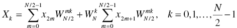
Further simplification is possible due to periodic and symmetric properties of the DFT as follows:
Thus, (7.20) is rewritten as follows:

Now, we define the FFT butterfly structure consisting of multiplication, addition, and subtraction as shown in Figure 7.5.

Figure 7.5 FFT butterfly
Simpler form is represented as shown in Figure 7.6.

Figure 7.6 Simple form of FFT butterfly
As we can observe from Figures 7.5 and 7.6, an N point DFT is divided into two N/2 point DFTs. They are composed of the terms ![]() and
and ![]() . Thus, we priorly calculate and store the term
. Thus, we priorly calculate and store the term ![]() . Then, we calculate the terms
. Then, we calculate the terms ![]() and
and ![]() and use them for Xk and
and use them for Xk and ![]() calculation. This butterfly architecture reduces the complexity of the DFT. Two N/2 point DFTs require 2(N/2)2 complex multiplies and 2(N/2) complex additions. Thus, the total number of the complexity is approximately N2/2. This is very meaningful result because the complexity has approximately halved through rearranging the equations. Figure 7.7 illustrates an example of a 8-point FFT structure based on butterfly.
calculation. This butterfly architecture reduces the complexity of the DFT. Two N/2 point DFTs require 2(N/2)2 complex multiplies and 2(N/2) complex additions. Thus, the total number of the complexity is approximately N2/2. This is very meaningful result because the complexity has approximately halved through rearranging the equations. Figure 7.7 illustrates an example of a 8-point FFT structure based on butterfly.

Figure 7.7 8-point FFT structure based on butterfly
We can further reduce the complexity using periodic and symmetric properties. In Equations 7.19 and 7.24, the N/2-point DFT ![]() is represented as follows:
is represented as follows:
and the N/2-point DFT ![]() is represented as follows:
is represented as follows:
where the twiddle factor ![]() is written as follows:
is written as follows:
Thus, (7.25) to (7.28) are rewritten as follows:
Figure 7.8 illustrates an example of 8-point FFT structure with further reduction.

Figure 7.8 8-point FFT structure with further reduction
In the same way, we keep splitting into even and odd terms M times (N = 2M). Thus, the N-point DFT is reconstructed by butterflies. Figure 7.9 illustrates an example of 8-point FFT structure consisting of butterflies only.

Figure 7.9 8-point FFT structure consisting of butterflies
In the N-point DFT, N is represented as follows:
where both r and M are integers. r is called the radix. When N is a power of 2, the type of the FFT is called a radix-2 FFT. In Figure 7.9, the radix-2 FFT is called decimation-in-time FFT. When observing the input of Figure 7.9, the input sequences are shuffled as [x0, x4, x2, x6, x1, x5, x3, x7]. We can implement this address order using the bit reversal as shown in Table 7.2.
Table 7.2 Bit reversal
| Binary (decimal) | Bit reversal (decimal) |
| 000 (0) | 000 (0) |
| 001 (1) | 100 (4) |
| 010 (2) | 010 (2) |
| 011 (3) | 110 (6) |
| 100 (4) | 001 (1) |
| 101 (5) | 101 (5) |
| 110 (6) | 011 (3) |
| 111 (7) | 111 (7) |
For IFFT derivation, (7.12) is rewritten using twiddle factors as follows:

The difference is a negative power of the twiddle factor and a multiplication factor (1/N). Thus, the FFT can be simply modified to the IFFT and the complexity of the IFFT increases as much as additional multiplication (1/N).
For decimation-in-frequency FFT derivation, we firstly divide the input sequence into two groups ([x0, x1, …, xN/2−1] and [xN/2, xN/2+1, …, xN−1]) and split (7.15) into two parts as follows:

and

For even index (k = 2m), we rewrite (7.34) using index shifting and periodic property as follows:
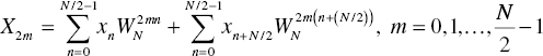

As we can observe from (7.39), the DFT output sequence with even index can be obtained as N/2 DFT of ![]() . For odd index (k = 2m + 1), we rewrite (7.37) using index shifting and periodic and symmetric properties as follows:
. For odd index (k = 2m + 1), we rewrite (7.37) using index shifting and periodic and symmetric properties as follows:


As we can observe from (7.41), the DFT output sequence with odd index can be obtained as N/2 DFT of ![]() . Similar to decimation-in-time butterfly, we can define the decimation-in-frequency FFT butterfly structure consisting of multiplication, addition, and subtraction as shown in Figure 7.11.
. Similar to decimation-in-time butterfly, we can define the decimation-in-frequency FFT butterfly structure consisting of multiplication, addition, and subtraction as shown in Figure 7.11.

Figure 7.11 Decimation-in-frequency FFT butterfly
Simpler form is represented as shown in Figure 7.12.

Figure 7.12 Simple form of decimation-in-frequency FFT butterfly
Figure 7.13 illustrates an example of the decimation-in-frequency 8-point FFT structure based on butterfly.

Figure 7.13 Decimation-in-frequency 8-point FFT structure
In the same way, we keep dividing and splitting so that the N-point DFT is reconstructed by butterflies. Figure 7.14 illustrates an example of the decimation-in-frequency 8-point FFT structure consisting of butterflies only.

Figure 7.14 Decimation-in-frequency 8-point FFT structure consisting of butterflies
Figure 7.15 Summary of radix-2 decimation-in-frequency 8-point FFT calculation
7.3 Hardware Implementations of FFT
When implementing the FFT block, many design issues such as complexity, latency, power, and memory should be considered. In 1970s, intensive researches about the FFT architecture were carried out. The Cooley–Tukey’s FFT algorithm [8] is widely used for developing FFT architectures. Since then, many different types of FFT architectures have been developed. Pipelined architectures such as the radix-2 single-path delay feedback (R2SDF) [9] and the radix-2 multi-path delay commutator (R2MDC) [10] allow us to develop a high-speed FFT. Thus, it is suitable for a broadband communication system. The pipelined FFT architecture can be classified in parallelism and data flow. According to both parallelism and data flow, the complexity and latency of the FFT are decided. As we discussed in the previous section, there are two types of FFT architectures: the decimation-in-time FFT and the decimation-in-frequency FFT. Their hardware implementation is different each other. We can intuitively build two architectures (the decimation-in-time FFT and the decimation-in-frequency FFT) by signal flow. Figure 7.16 illustrates the radix-2 decimation-in-time 8-point FFT signal flow graph and hardware architecture. In the first stage, signal elements are paired ((x0 x4), (x2 x6), (x1 x5), and (x3 x7)). One element (x4, x6, x5, and x7) of the pair is multiplied by the twiddle factor. Then, they become inputs of the butterfly. In the second stage, the outputs of the butterfly in the first stage are rearranged and paired to become inputs of the second stage butterfly ![]() . In the third stage, the outputs of the FFT (X0, X1, X2, X3, X4, X5, X6, and X7) can be obtained by rearranging the inputs
. In the third stage, the outputs of the FFT (X0, X1, X2, X3, X4, X5, X6, and X7) can be obtained by rearranging the inputs ![]() and calculating the butterfly. In the same way, we calculate the radix-2 decimation-in-frequency 8-point FFT as shown in Figure 7.17. In the first stage, one element (x4, x5, x6, and x7) of the signal pair is multiplied by twiddle factor. The paired signals ((x0 x4), (x1 x5), (x2 x6), and (x3 x7)) become inputs of the butterfly. In the second stage, the rearranged signal pairs
and calculating the butterfly. In the same way, we calculate the radix-2 decimation-in-frequency 8-point FFT as shown in Figure 7.17. In the first stage, one element (x4, x5, x6, and x7) of the signal pair is multiplied by twiddle factor. The paired signals ((x0 x4), (x1 x5), (x2 x6), and (x3 x7)) become inputs of the butterfly. In the second stage, the rearranged signal pairs ![]() are calculated by the butterfly. In the third stage, the output of the FFT (X0, X4, X2, X6, X1, X5, X3, and X7) can be obtained by rearranging the inputs
are calculated by the butterfly. In the third stage, the output of the FFT (X0, X4, X2, X6, X1, X5, X3, and X7) can be obtained by rearranging the inputs ![]() and calculating the butterfly. These two architectures are designed in signal flow point of view. We need to consider efficiently using parallelism and memory usage when implementing FFT architectures. Thus, we look into the R2SDF and R2MDC in this section.
and calculating the butterfly. These two architectures are designed in signal flow point of view. We need to consider efficiently using parallelism and memory usage when implementing FFT architectures. Thus, we look into the R2SDF and R2MDC in this section.

Figure 7.16 Radix-2 decimation-in-time 8-point FFT signal flow graph and hardware architecture

Figure 7.17 Radix-2 decimation-in-frequency 8-point FFT signal flow graph
Figure 7.18 illustrates the radix-2 single-path delay feedback.

Figure 7.18 Radix-2 single-path delay feedback.
The R2SDF has a single data path going through the butterfly and multiplier and a delay line arranging input pairs of the butterfly. Each stage has different delays (Delay 4, Delay 2, and Delay 1) which arrange the input pairs as follows: In the first stage, the first half of the delayed signal (x7, x6, x5, and x4) is paired with the second half of the original signal (x3, x2, x1, and x0). In the second stage, four elements of the delayed signal ![]() are paired with the four elements of the original signal
are paired with the four elements of the original signal ![]() . In the third stage, four elements of the delayed signal
. In the third stage, four elements of the delayed signal ![]() are paired with the four elements of the original signal
are paired with the four elements of the original signal ![]() . Table 7.3 summarizes the signal flow of the R2SDF.
. Table 7.3 summarizes the signal flow of the R2SDF.
Table 7.3 Signal flow of R2SDF
| Stage 1 | ||
| Delay 4 | Butterfly | |
| x7, x6, x5, x4, x3, x2, x1, x0 | x7, x6, x5, x4, x3, x2, x1, x0 x7, x6, x5, x4, x3, x2, x1, x0 |
|
| Stage 2 | ||
| Delay 2 | Butterfly | |
| Stage 3 | ||
| Delay 1 | Butterfly | |
| X0, X4, X2, X6, X1, X5, X3, X7 | ||
The delay line is simply implemented by shift registers. In order to reduce power consumption and area, SRAM can be used. Thus, it can perform the read and write operation in one clock cycle [11]. The R2SDF can efficiently use the registers. However, it is not convenient to implement a large size FFT because it requires a large size shift register and a high power is consumed by shifting a large size data.
The R2MDC uses two parallel data paths which are calculated in one butterfly. Figure 7.19 illustrates the radix-2 multi-path delay commutator. As we can observe from the figure, there is no feedback. Thus, it can be implemented using more pipelining and parallel processing techniques.
Figure 7.19 Radix-2 multi-path delay commutator
Table 7.4 summarizes the signal flow of the R2MDC. In the first stage, the switch sends the first signal (x3, x2, x1, and x0) to upper signal line and is delayed. The upper signal line is aligned with the second half of the lower signal line (x7, x6, x5, and x4). In the second stage, the lower signal line is delayed and the second half is switched with the upper signal line ![]() . Then, the upper signal line is delayed and aligned with the lower signal line. In the third stage, the lower signal line is delayed and two signal elements are switched with the upper signal line
. Then, the upper signal line is delayed and aligned with the lower signal line. In the third stage, the lower signal line is delayed and two signal elements are switched with the upper signal line ![]() . Then, the upper signal line is delayed and aligned with the lower signal line. Finally, we obtain the output of the FFT. As we can observe Figure 7.19 and the Table 7.4, the butterfly in the first stage is not working until signals are paired. Thus, the hardware utilization rate of the R2MDC is 50%. For increasing the data throughput, the radix-4 multipath delay commutator can be used. This architecture can achieve higher data throughput due to four parallel data path but the hardware utilization rate is only 25%. Thus, the data throughput and the hardware utilization are trade-off relationship. One possible solution to increase both metrics is to use the duplicated input. That is to say the input signal is duplicated. The duplicated signal is aligned with the original signal. They are put into the FFT simultaneously with delay.
. Then, the upper signal line is delayed and aligned with the lower signal line. Finally, we obtain the output of the FFT. As we can observe Figure 7.19 and the Table 7.4, the butterfly in the first stage is not working until signals are paired. Thus, the hardware utilization rate of the R2MDC is 50%. For increasing the data throughput, the radix-4 multipath delay commutator can be used. This architecture can achieve higher data throughput due to four parallel data path but the hardware utilization rate is only 25%. Thus, the data throughput and the hardware utilization are trade-off relationship. One possible solution to increase both metrics is to use the duplicated input. That is to say the input signal is duplicated. The duplicated signal is aligned with the original signal. They are put into the FFT simultaneously with delay.
Table 7.4 Signal flow of radix-2 multi-path delay commutator
| Stage 1 | |||
| Switch | Delay 4 | Butterfly | |
| x7, x6, x5, x4, x3, x2, x1, x0 | x3, x2, x1, x0 | x3, x2, x1, x0 | |
| x7, x6, x5, x4 | x7, x6, x5, x4 | ||
| Stage 2 | |||
| Delay 2 | Switch | Delay 2 | Butterfly |
| Stage 3 | |||
| Delay 1 | Switch | Delay 1 | Butterfly |
| X0, X4, X2, X6, X1, X5, X3, X7 | |||
7.4 Problems
- 7.1. Consider an OFDM system with 1024 subcarriers (768 data, 83 pilots, and 173 guard subcarriers), subcarrier spacing = 125 Hz, guard interval = 1 ms, and QPSK modulation. Find the bandwidth and data rate of the OFDM system.
- 7.2. Consider an OFDM system with 128 subcarriers (96 data, 9 pilots, and 23 guard subcarriers), bandwidth = 1 MHz, bandwidth efficiency = 0.9 and 16QAM modulation. Find the data rate of the OFDM system.
- 7.3. Compare the PAPRs of an OFDM system with 128 and 1024 DFT size.
- 7.4. There are many PAPR reduction techniques such as clipping and filtering, block coding, interleaving, tone reservation, tone injection, selective mapping, and partial transmit sequences. Compare their advantages and disadvantages.
- 7.5. Compare the performance of zero padding and cyclic prefix.
- 7.6. Mobile WiMAX supports scalable channel bandwidths and adopts scalable OFDMA (SOFDMA). SOFDMA adjusts the DFT/IDFT size while subcarrier spacing is fixed. Describe the advantages and disadvantages of the SOFDMA.
- 7.7. Consider the following design requirements and design the OFDM system:
Requirements Values Speed 120 km/h Carrier frequency 3.5 GHz Tolerable delay spread 20 µs Bandwidth 1 MHz Target data rate 2 Mbps - 7.8. Consider the following input sequence:

- 7.9. Calculate the output sequences of the radix-2 8-point FFT, radix-2 decimation-in-frequency 8-point FFT and DFT and then compare them.
References
- [1] H. Yaghoobi, “Scalable OFDMA Physical Layer in IEEE802.16 Wireless MAN,” Intel Technology Journal, vol.8, no. 3, pp. 201–212, 2004.
- [2] Y. Li and L. J. Cimini, “Bounds on the Interchannel Interference of OFDM in Time Varying Impairments,” IEEE Transactions on Communications, vol. 49, no.3, pp. 401–404, 2001.
- [3] IEEE802.16 Broadband Wireless Access Working Group, “Channel Models for Fixed Wireless Application.” Revision 4.0, IEEE802.16.3c-01/29r4, July 2001.
- [4] ITU-R Recommendation M.1225, “Guidelines for Evaluation of Radio Transmission Technologies for IMT-2000, 1997.” Feburary 1997. http://www.itu.int/rec/R-REC-M.1225/en (accessed April 20, 2015).
- [5] R. V. Nee and R. Prasad, “OFDM for Wireless Multimedia Communications,” Artech House Publishers, Boston, MA, 2000.
- [6] P. Hoeher, S. Kaiser, and P. Robertson, “Two-dimensional Pilot-Symbol-Aided Channel Estimation by Wiener Filtering,” Proceedings of IEEE International Conference on Acoustics, Speech, and Signal Processing 1997 (ICASSP-97), vol. 3, pp. 1845–1848, April 1997.
- [7] R. Negi and J. Cioffi, “Pilot Tone Selection for Channel Estimation in a Mobile OFDM System,” IEEE Transactions on Consumer Electronics, vol. 44, no. 3, pp. 1122–1128, 1998.
- [8] J. W. Cooley and J. Tukey, “An Algorithm for Machine Calculation of Complex Fourier Series,” Mathematics of Computation, vol. 19, no. 90, pp. 297–301, 1965.
- [9] H. L. Groginsky and G. A. Works, “A Pipeline Fast Fourier Transform,” IEEE Transactions on Computers, vol. c-19, no. 11, pp. 1015–1019, 1970.
- [10] L. R. Rabiner and B. Gold, Theory and Application of Digital Signal Processing, Prentice-Hall, Englewood Cliffs, NJ, 1975.
- [11] Y. T. Lin, P. Y. Tsai, and T. D. Chiueh, “Low-power Variable Length Fast Fourier Transform Processor,” IEE Proceedings Computers and Digital Techniques, vol. 152, no. 4, 2005.