Chapter 2
Theory of WPT
2.1. Theoretical background
The following four Maxwell’s equations can describe all electromagnetic phenomena such as radiowaves and light:
where H, B = μH, E, D = εE, J = σE and ρ indicate magnetic field (A/m), magnetic flux density (T), electric field (V/m), electric flux density (C/m2), current density (A/m2) and charge density (C/m3), respectively. μ, ε and σ indicate magnetic permeability (H/m), permeability (F/m) and electrical conductivity (1/Ω·m), respectively. Maxwell’s equations indicate that electromagnetic waves propagate in a field based on relationships between the electric field, magnetic field, time and space.
It is known that electromagnetic energy is also associated with the propagation of electromagnetic waves. The energy of electromagnetic waves can be described as E×H (W/m2). The vector E×H is called the Poynting vector. In plane wave propagation, the vector E×H results in a vector along the direction of propagation, which is same as the direction of the energy flow. It means that all electromagnetic waves themselves are energy. Theoretically, we can use all electromagnetic waves for wireless power transfer (WPT). Maxwell’s equations indicate that the electromagnetic field and its power diffuse in all directions. Although we transmit energy in a communication system, the transmitted energy is diffused in all directions. WPT and wireless communication systems fundamentally differ only in how radiowaves are used by the receiver. In wireless communication systems, information is imparted to the transmitted radiowave via modulation. The radiowave is only a carrier of the information and is not very important itself. In contrast, for WPT systems, the radiowave itself is important and is used after rectifying. In wireless communication systems, the modulated radiowave is demodulated by a receiver. For WPT systems, the radiowave is rectified; in other words, it is converted from a high-frequency wave (greater than kilohertz) to a low-frequency wave (several tens of hertz) or DC.
2.2. Beam efficiency and coupling efficiency
2.2.1. Beam efficiency of radiowaves
An antenna is used to transmit and receive radiowaves. The antenna is a resonator at a selected frequency and is a converter of the radiowave from a circuit to free space (transmitting) and to a circuit from free space (receiving). The antenna is composed of metals and dielectric materials, whose shape and electric parameters decide the resonant frequency. Antennas are typically used for wireless communication and for radar and remote sensing. Identical antennas can also be used for WPT. Design theory and technologies are basically the same whether antennas are for wireless communication, radar, remote sensing or WPT.
The power of a radiowave is wirelessly transmitted from a transmitting antenna to a receiving antenna. It is a straightforward exercise to use the Friis transmission equation for calculating the receiving power at a far-field distance given as follows:
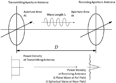
where Pr, Pt, Gr, Gt, Ar, At, λ and D are the received power, transmitted power, antenna gain of the receiving antenna, antenna gain of the transmitting antenna, aperture area of the receiving antenna, aperture area of the transmitting antenna, wavelength, and the distance between the transmitting antenna and the receiving antenna, respectively (Figure 2.1). The Friis transmission equation assumes plane waves under sufficiently far-field conditions. The Friis transmission equation can be used to calculate the receiving power at far field for energy harvesting or for WPT using diffused radiowaves.
However, we cannot use the Friis transmission equation for a WPT application by using beamed radiowaves because we must calculate the receiving power at a distance in the near field. A spherical wave is generated in the near field where beamed WPT is applied.
Therefore, we use the following τ parameter to calculate the receiving power or beam efficiency (BE) η [GOU 61, BRO 73a, ITU 00].
It is assumed that the amplitude and the phase of a radiowave are uniform at the transmitting antenna, as shown in Figure 2.1. It is also assumed that the transmitting antenna and the receiving antenna are at the correct position.
Figure 2.1. Transmitting antenna and receiving antenna
From equation [2.6], it can be observed that τ2 represents the BE calculated by the Friis transmission equation [2.5] in the far field. Equation [2.7] indicates that, for a given frequency and distance, a large aperture antenna must be used to increase the BE. The BE in the far field and the near field using the τ parameter is shown in Figure 2.2. We can increase the BE approximately to 100% with τ > 2 in the near field. The theory does not depend on power. Therefore, we can transmit high power via radiowaves. For small τ, the BE obtained is almost the same from both formulas, and under those conditions, we can assume a plane wave in the far field. When the distance between the transmitting antenna and the receiving antenna is shortened, τ becomes larger and we cannot assume a plane wave at the receiving antenna plane, and therefore we cannot use the Friis transmission equation.
Figure 2.2. Beam efficiency in the far field and the near field using the τ parameter

Equation [2.7] is an approximation that neglects sidelobes. We can calculate the BE exactly by including the near-field beam pattern. Figure 2.3 shows the BE of a WPT system, e.g. the wireless charging of an electric vehicle, where f, Tx and Rx are frequency, the diameter of the transmitting antenna and the diameter of the receiving antenna, respectively. The BE is 90% at a distance of <5 m for standard WPT parameters. Therefore, the efficiency of WPT via radiowaves is sufficiently high relative to resonant or inductive coupling.
Figure 2.3. Beam efficiency of WPT system without approximation

The use of microwaves is essential to realize τ > 2 because τ is inversely proportional to the wavelength. The first WPT experiment conducted by Nicola Tesla in the early 20th Century had a drawback of low BE because he used 150 kHz radiowaves. In the 1960s, Brown’s WPT experiments succeeded because he used microwaves in the gigahertz range having a high BE as the wavelength of microwaves is much shorter than that of 150 kHz radiowaves. However, DC–RF conversion and RF–DC conversion efficiencies decrease at higher frequencies. Therefore, the total efficiency of WPT via microwaves is approximately 50%, which includes DC–RF conversion efficiency, BE, absorption efficiency of the antenna and the RF–DC conversion efficiency.
2.2.2. Theoretical increase of beam efficiency
From a theoretical perspective, we cannot increase the BE in the manner indicated by equation [2.7], but we can increase the BE by changing the power distribution on the transmitting antenna. We assume that the power distribution on the transmitting antenna is uniform in equation [2.7], as shown in Figure 2.1. A well-known power distribution exists that will enable us to increase the BE, which can be described with the following formula.
1) Gaussian power distribution
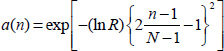
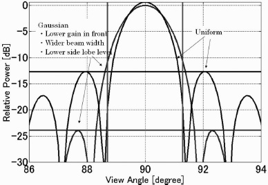
where a(n) is the power distribution on the transmitting antenna, R is the ratio between the power at the center and at the edge of the transmitting antenna, n is the index of an antenna element and N is total number of antenna elements. In equation [2.8], we assume that an aperture antenna can be considered as a sum of antenna elements of a sufficient number N, which is a description of a phased array. It is standard to call a distribution “10 dB Gaussian power distribution” when the value of R is 10 dB. The beam pattern created by the Gaussian power distribution has a lower gain and wider beam width than that created by a uniform power distribution. As a result, the BE determined by the Gaussian power distribution increases relative to that by the uniform power distribution. The beam patterns of Gaussian power distributions and uniform power distributions at far field are shown in Figure 2.4. The Gaussian power distribution is often adopted in a solar power satellite (SPS) design to increase the BE.
2) Chebyshev power distribution

where R is the ratio between the power at the center and the power at the edge of the transmitting antenna, n is the index of an antenna element, N is total number of the antenna elements and

Figure 2.4. Comparison of beam patterns at far field between a Gaussian power distribution and a uniform power distribution
The beam pattern created by a Chebyshev power distribution is formulated as follows:
where dn is the element spacing and
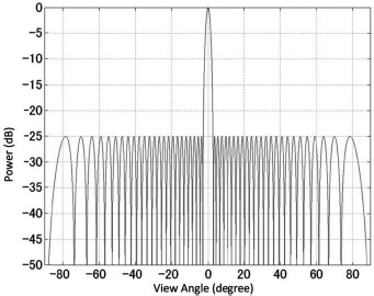
Figure 2.5 illustrates a beam pattern at far field created by the Chebyshev power distribution with N = 50 and R = 25 dB. It is a characteristic of the beam pattern generated by the Chebyshev power distribution that all sidelobe levels are the same. The first sidelobe level is suppressed, but the other sidelobe levels are increased.
Figure 2.5. Beam pattern at far field created by the Chebyshev power distribution with N = 50 and R = 25 dB
3) Taylor power distribution
where

where
g(u): directivity from the uniform power distribution;
ucm: mth null point from the Chebyshev power distribution;
ugm: mth null point from the uniform power distribution;
![]() : same number of null points derived from the Chebyshev power distribution.
: same number of null points derived from the Chebyshev power distribution.
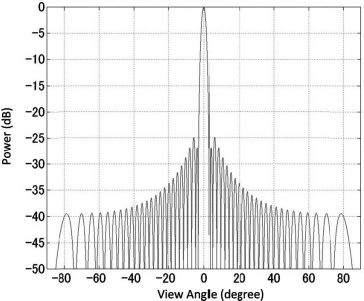
The Taylor power distribution is a combination of the Chebyshev and the uniform power distributions. Sidelobe levels that are closer to a main lobe than the mth number are similar to that from the Chebyshev power distribution. A beam pattern at far field created by the Taylor power distribution with N = 50, sidelobe levels of –25 dB and ![]() = 1 is shown in Figure 2.6.
= 1 is shown in Figure 2.6.
Figure 2.6. Beam pattern at far field created by the Taylor power distribution with N = 50, sidelobe levels of –25 dB and ![]() = 1
= 1
2.2.3. Coupling efficiency at very close coupling distance
We usually use antennas at near field or far field for WPT via radiowaves. High frequencies in the megahertz to gigahertz range are beneficial to effectively transmit wireless power. If we use lower frequencies in the range of less than a kilohertz, it is difficult to make use of the WPT system even at near field. A distance closer than near field is referred to as the reactive field. At the reactive field, we should consider not an electromagnetic wave but an electric field or a magnetic field alone. When we use a coil as a closed loop, the coil creates a magnetic field and the magnetic field transfers wireless power. This is inductive coupling WPT. Inductive coupling WPT is based on Ampère’s circuital law and Faraday’s law of induction. Ampère’s law and Faraday’s law of induction are approximations of Maxwell’s equations. Ampère’s circuital law describes the relationship between the integrated magnetic field around a closed loop (coil) and the electric current passing through the loop. Faraday’s law of induction describes the relationship between a time-varying magnetic field and an induced electric field. The electric power is carried through the magnetic field between two coils. Ampère’s circuital law and Faraday’s law of induction are both examples of Maxwell’s equations. The efficiency of WPT depends on the coupling coefficient, which in turn depends on the distance between the two coils. Therefore, wireless energy cannot be carried over a distance longer than a few millimeters with high efficiency using inductive coupling, and the frequency used in inductive coupling is below a few dozen megahertz.
When we add a capacitor of a capacitance (C) to a coil that is defined by an inductance (L), the two elements form a resonator having properties defined by both C and L. When two resonators are electromagnetically coupled, the energy in one resonator is transmitted to the other through an evanescent mode wave. This phenomenon is well known as coupling theory applied to a microwave band pass filter. However, it was not until 2006 that Massachusetts Institute of Technology (MIT) researchers demonstrated a WPT experiment using resonant coupling. Resonant coupling with coils is called magnetic resonant coupling. The transmitted power is mainly a magnetic field supported by a coil. Resonant coupling is realized with two plane-shaped conductors passing through an electric field and is called electric resonant coupling.
A transmitting antenna and a receiving antenna are usually not coupled, and wireless power is transferred between them through space. Two coils or two resonators, however, are electromagnetically coupled for inductive coupling WPT and resonant coupling WPT systems. A theoretical investigation based mainly on inductive coupling has been conducted for magnetic resonant coupling. From the theory of inductive coupling, k·Q, where k is the coupling coefficient and Q is the quality factor of the coil resonator, is the critical factor established. The maximum coupling transmission efficiency η is calculated using k·Q, as shown in the following equations.

where ω is the frequency, R is the resistance and M is the mutual inductance. The efficiency curve is shown in Figure 2.7. The coupling transmission efficiency is determined by k·Q. In inductive coupling, a high Q factor cannot be used; therefore, k should increase as a function of the distance between the two coils. However, in resonant coupling, it is easy to increase k·Q with a high Q factor even if the distance between the two coils is large and the k factor is small (note that k contains a wavelength parameter). If a lower frequency is selected, then k increases if the distance and Q factor are the same. As a result, the WPT distance having a high efficiency is expanded using a lower frequency in an inductive or resonant coupling WPT system. A lower frequency indicates that higher efficiency can be achieved using lower cost components for the system.
Figure 2.7. Coupling transmission efficiency of inductive coupling and resonant coupling

2.3. Beam forming
2.3.1. Beam-forming theory for the phased array and its error
Equation [2.18] includes a parameter reflecting the positions of the resonators or coils in k. The value of k includes not only the positions, but also the distance between the two resonators or two coils. Equation [2.6] or [2.7] includes a parameter reflecting the distance between two antennas but does not include the positions of the two antennas. The easiest way to maintain a high BE is to control the direction of the antenna and maintain the correct position. However, we have to mechanically control the direction of the antenna, which is not an easy task.
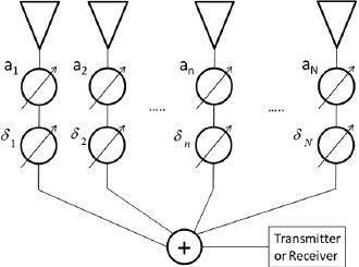
A phased array antenna is a useful piece of technology for electrically controlling the beam direction. The phased array is composed of plural antennas as shown in Figure 2.8. We control the phase and the amplitude of the radiowave transmitted at each antenna with phase shifters or a beam-forming network circuit. A beam form is controlled by interference of the radiowaves (Figure 2.9). To calculate the beam pattern from a phased array, we need r (the distance between a transmitting antenna element and a receiving point), θ and ϕ (the two angles acting between a transmitting antenna element and a receiving point) and D(r, θ, ϕ) (the element pattern of the transmitting antenna element). All antenna elements have a peculiar element pattern (directivity) D(r, θ, ϕ).
Figure 2.8. Concept of a phased array I

The calculation method of the phased array shown in Figure 2.9 can be used both in near field and far field. However, it is difficult to calculate the beam form. Therefore, at far field, we can omit the distance parameter r and use the following equation to calculate the beam form E(θ,ϕ). It is based on consideration of the “array factor”. The array factor A(θ,ϕ) collectively indicates the directivity of all antenna elements, which considers the phased array as an aperture array. We can calculate the beam form E(θ,ϕ) as the product of the element factor D(θ,ϕ) and the array factor A(θ,ϕ) at far field.
Figure 2.9. Concept of a phased array II

The array factor is determined by the antenna elements by their positions, amplitude and phase, and is not related to the types of antennas used. When we consider a one-dimensional (1D) uniformly spaced array of N antenna elements, the array factor is given as follows:
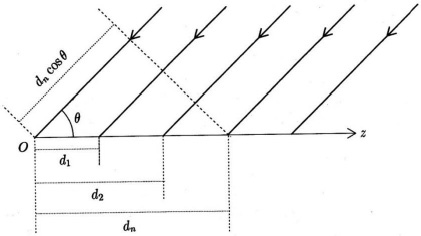
where an and ϕn are the amplitude and the phase of nth antenna element, respectively. The parameters are shown in Figure 2.10. Equation [2.19] is transformed using equation [2.19] to obtain the following equation:
Figure 2.10. Parameters of array used to calculate the beam form at far field
The phase of an antenna element is caused by the difference of the antenna position and a phase shifter that can arbitrarily control the phase. The phase of the nth element can be geometrically described as ϕn = kdn cosθ + δn, where k is the wave number, dn is the nth element spacing and δn is an additional phase shift, for example, caused by a phase shifter. Equation [2.21] can be described using ϕn as follows:
The parameters describing a phased array are shown in Figure 2.11. The relationships between the beam form of a phased array, element factor and array factor are shown in Figure 2.12. It is easy to calculate the beam form at far field using equation [2.22].
Figure 2.11. Parameters of a uniform spacing array used to calculate the beam form at far field
Next, when we give an equal interval phase at each phase shifter for a uniform spacing array, in other words, when we assign phases of 0, δ, 2δ, …, (n – 1)δ at each phase shifter, the array factor A(ψ) is given as follows:
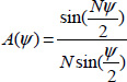
where an is equal to 1 and ψ is an angle. The beam form using A(ψ) is shown in Figure 2.13 when a phase standard point is at the center of the array and the amplitude is standardized by a maximum corresponding to a magnitude of 1. The figure corresponds to a beam form from an aperture antenna with a uniform power distribution. Sidelobes are also shown.
Figure 2.12. Relationships between the beam form of a phased array, element factor and array factor

Figure 2.13. Beam form of uniform spacing array

The direction of maximum beam power θmax is given by equation [2.22] as follows:
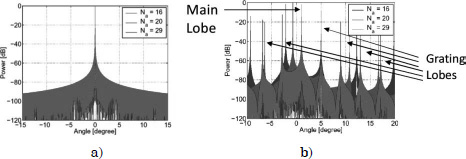
Equation [2.24] contains a sinusoidal function. It is easy to understand that a lot of solutions are realized from equation [2.24]. This equation indicates that a number of intense beam points will occur when an equal interval phase is given at each phase shifter in a uniform spacing array. This is called a grating lobe, whose power is the same as the main beam. Figures 2.14(a) and (b) show the two beam forms of a 1D uniform spacing array. Na corresponds to an element spacing d. A large Na corresponds to a large d. Figure 2.14(a) shows a beam form where the phase at all phase shifters is 0. The beam is focused at the center of the array. Figure 2.14(b) shows a beam form wherein we assign an equal interval phase at each phase shifter to focus the beam at an angle of 5°. In Figure 2.14(b), we can see that grating lobes arise. Power is distributed to all grating lobes when grating lobes arise. It is clear that grating lobes should be suppressed in order to realize high BE for the WPT system.
Figure 2.14. Beam form of a 1D phased array: a) focus direction: 0°, b) focus direction: 5°. For a color version of this figure, see www.iste.co.uk/shinohara/radiowaves.zip
The condition of no grating lobes is given by the following equation:
where θs is the focused direction angle, d is the element spacing and λ is the wavelength. For example, θs < 19.5o when d = 0.75λ and θs < 41.8o when d = 0.6λ. No grating lobes arise in the condition d < 0.5λ. If d > λ, grating lobes must rise except in the case θs = 0o, i.e. for a front beam.
Phased array and beam-forming theories do not account for phase/frequency/amplitude error. The efficiency of the array must decrease owing to phase/frequency/amplitude error. Phase/frequency/amplitude error for a phased array causes differences in beam direction and the rise of sidelobes. Differences in the beam direction caused by phase errors are described by the following equation:
where ΔB is the change in the beam direction, N is number of phased array elements and Δϕ is the maximum antenna element phase error. For a sufficiently large number of elements, the change in the beam direction is negligible. For example, assuming N = 10,000 in one dimension and Δϕ = 5° in the SPS case, ΔB is 1.732 × 10‒5º or 10.9 m at a distance of 36,000 km.
A more serious problem for the decline in the beam collection efficiency is the rise of sidelobes caused by phase/frequency/amplitude error. The following equation defines the mean squared sidelobe level (MSSL) by means of the probability of antenna element trouble (PT), dispersion of the amplitude error ![]() dispersion of the phase error
dispersion of the phase error ![]() , aperture efficiency (ηa) and the number of elements (N) [SKO 90].
, aperture efficiency (ηa) and the number of elements (N) [SKO 90].
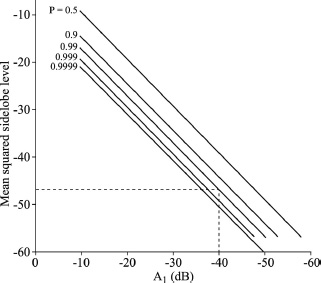
The MSSL indicates an average error sidelobe level caused by antenna element trouble and errors in amplitude and phase. It is assumed that the MSSL results in power leakage from the main lobe and is the average sidelobe level in all directions. The MSSL must be added on an original sidelobe level without any errors in order to know the real sidelobe level with the errors. The MSSL gives a probability (P) that there is no sidelobe over a value RT as shown in the following equation:
For example, when the MSSL is –47 dB, the probability is 0.99 that sidelobes do not rise above –40 dB (Figure 2.15).
Figure 2.15. Sidelobe level to be held with probability P [SKO 90]
The rise of sidelobes decreases the antenna gain and beam collection efficiency. The antenna gain (G) with probability of antenna element trouble (PT), dispersion of amplitude error ![]() and dispersion of phase error
and dispersion of phase error ![]() can be described as follows [MAI 94]:
can be described as follows [MAI 94]:
where G0 is the antenna gain without any errors.
If antenna planes structurally separate from each other, grating lobes, whose power levels are the same as the main beam, may occur and power may not be effectively concentrated to the rectenna array. This problem occurs in module-type phased arrays. The idea of a random array has been investigated as a means of suppressing grating lobes. However, as the sidelobe level increases, beam collection efficiency decreases and then special techniques are required. The power of grating lobes diffuses not to the main lobe but to the sidelobes. Therefore, we have to fundamentally suppress grating lobes for an efficient microwave power transfer (MPT) system.
2.3.2. Target detecting via radiowaves
Control of the direction of a power beam is of no significance if we cannot detect the receiving target. There are various target detection methods: global positioning system (GPS); optical detection; direction-of-arrival (DOA) methods, such as multiple signal classification (MUSIC) via radiowaves; and a method named retrodirective detection, which uses a pilot signal radiowave. In the microwave lifted airplane experiment (MILAX) experiment shown in Figure 1.7, optical target detection was accomplished using two charge coupled device (CCD) cameras. The difference between the retrodirective method and other target detection methods is that only the former can detect both the positions of the target and antenna elements (the shape of the antenna array) in a phased array.
Use of radiowaves as pilot signals to detect the receiving target has been made in various MPT field experiments. In certain MPT experiments, a DOA algorithm with a pilot signal and phase shifters controlled by the DOA algorithm were used to implement a phased array. The minimum configuration of a DOA radiowave array is a two-antenna system, as shown in Figure 2.16. The DOA angle θ can be estimated from the phase difference between the two antennas Δθ, element spacing d and wavelength λ as follows:
Figure 2.16. Fundamental direction of arrival of radiowave

After the estimation of the DOA angle, each phase of the antennas is estimated. A power beam is created with the phased data and is sent back to the detected source. Phase shifters must be used to control the beam produced by each antenna in typical phased arrays. For optimum beam forming in a phased array, various methods such as neural networks, genetic algorithms and multiobjective optimization learning are available. The term “optimum” has multiple meanings: to suppress sidelobe levels, to increase beam collection efficiency and to produce multiple power beams. Array optimization can be freely implemented by considering system complexity and the calculation time required by the control algorithm. Such DOA systems that use control algorithms are sometimes called “software retrodirective” systems.
However, an error occurs in DOA estimation because of the signal/noise (SN) ratio. The estimation error Δθ′ is formulated as follows [LIP 87]:
DOA estimation errors calculated by equation [2.35] for various SN ratios are shown in Figure 2.17. DOA estimation errors should be considered in the design of an MPT system. If more than two antennas are used, SN ratio of the system decreases. An advanced algorithm, such as MUSIC, can also be applied to implement the DOA. The algorithm can decrease SN ratio, thus increasing the target detection accuracy.
On the other hand, phase shifters are not used in a retrodirective system. A pilot signal originating from the target is used in both retrodirective and software retrodirective systems. A corner reflector is the most basic retrodirective system [SUN 03]. Corner reflectors consist of perpendicular metal sheets jointed at the apex (Figure 2.18(a)). Incoming signals are reflected back in the DOA through multiple reflections off the reflector wall. The Van Atta array is another basic retrodirective system [VAN 59]. It is made up of pairs of antennas equidistantly spaced from the center of the array and connected with equilength transmission lines (Figure 2.18(b)). The signal received by an antenna is re-radiated by its pair; thus, the order of re-radiating elements is inverted with respect to the center of the array, achieving proper phasing for retrodirectivity.
Figure 2.17. Estimation error of DOA Δθ

Figure 2.18. a) Two-sided corner reflector, b) Van Atta array, c) retrodirective array with phase-conjugate circuits [SUN 03]

Usually, retrodirective systems have phase-conjugate circuits in each receiving/transmitting antenna (Figure 2.18(c)), which play the same role as the pairs of antennas spaced equidistantly from the center of the array in a Van Atta array. A pilot signal transmitted from the target (amplitude: VRF, angular frequency: ωRF and phase at each antenna: +θn) is received and re-radiated through the phase-conjugate circuit in the direction of the target. A local signal (amplitude: VLO and angular frequency: ωLO) is used for phase conjugation. Two forms of the pilot signal and the local signal are mixed and the conjugate signal VIF is obtained as defined by the following equation and as shown in Figure 2.19(a):
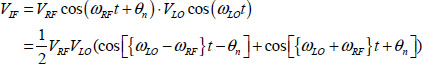
When a low-pass filter is used after mixing, the following signal is obtained. The phase + θn is changed to –θn:
If we choose ωLO = 2ωRF, equation [2.33] becomes:
as shown in Figure 2.19(b).
The accuracy of the sending direction depends on the stability of the frequency of the pilot signal and the local oscillator (LO) signal. To decrease a beam-forming error caused by the fluctuation of the LO signal, the same pilot signal and frequency doubler are used instead of the LO signal.
Figure 2.19. Block diagram of a retrodirective system with phase conjugation: a) output without filtering; b) output with low-pass filter (LPF)

2.4. Beam receiving
Equation [2.3] represents only the transfer efficiency. Therefore, we have to additionally consider the radiation or absorption efficiency of an antenna for WPT via radiowaves.
An infinite array can theoretically absorb 100% of a transmitted radiowave [DIA 68, STA 74]. In general, the infinite array model can approximately apply to the analysis of a large array. Although edge effects cannot be evaluated under such an approximation, very simple and useful results are obtained.
Itoh et al. calculated the absorption efficiency of a rectenna array composed of circular microstrip antennas (CMSA), as shown in Figure 2.20. The following analysis is referenced in [ITO 86]. An angle θ representing the direction of propagation of the incident plane wave is restricted to the x–z plane. Polarization is parallel to the x–z plane. Therefore, the polarization mismatch loss can be ignored. Here, it is assumed that the thickness of the substrate is very small as compared to the wave length. Therefore, a single-mode (TM110) excitation model of a magnetic current loop on the ground plane, a very simplified model, can be considered. Using Stark’s method [STA 74], the active admittance Y is obtained as follows:

where βm = 2πm/Lx + k sin θ, hn = 2πn/Ly,

k is the wave number of the indecent wave, and βm, hn and γmn are propagation constants of the space harmonic wave along x, y and z, respectively. Here higher waves correspond to grating lobes.
Figure 2.20. a) Circular microstrip antenna; b) geometry of infinite CMSA array [ITO 86]

When all higher waves are evanescent, the active conductance G is expressed using equation [2.35] as follows:
where ρ = ka sin θ.
The absorption efficiency of the infinite rectenna array is defined as the ratio of the maximum receiving power of an element to the incident power per element [ADA 81]. Then, the absorption efficiency ηabsorp is represented by:
Here, the numerator denotes the absorption cross-section. The denominator denotes the cross-section of the cell. The absorption cross-section Ae is given by:
where Grad and Da are the radiation conductance and the directivity of a single element, respectively, and G is the active conductance. Therefore, Ae is rearranged as follows:
where ρ = ka sin θ.
From equations [2.37] and [2.39], the absorption efficiency is obtained as follows:
When we consider the case of no grating lobes, the absorption efficiency ηabsorp becomes 100%, which is obtained by the substitution of equation [2.36] into equation [2.40]. This means that the infinite CMSA rectenna array can perfectly absorb the incident power under the condition of no grating lobes. This result is identical to that of a dipole antenna with a ground plane [ITO 84].
Figure 2.21 shows the absorption efficiency versus element spacing in the case of a square lattice (Lx = Ly = L). When the grating lobe is generated, the efficiency approaches zero because all the incident power flow is along the x–z plane or in the direction of propagation of the grating lobe. This phenomenon cannot be observed for an infinite array of dipoles with a ground plane in which the cancellation occurs between dipoles and their image [ITO 86]. However, the above discussion ignores the effect of the thickness of the substance. In fact, it is predicted that the efficiency is greater than zero because a surface wave generates before the formation of grating lobes.
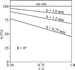
Figure 2.22 shows the absorption efficiency in consideration of ohmic and dielectric losses of the CMSA, where the relative dielectric constant of the substrate is 2.6 and tan δ is 2.2 × 10⁻³. The greater spacing provides a smaller efficiency.
Figure 2.21. Absorption efficiency versus element spacing, where the parameter is the incident angle θ (Lx = Ly = L) [ITO 86]

Figure 2.22. Absorption efficiency versus element spacing, where CMSA possesses ohmic and dielectric losses [ITO 86]
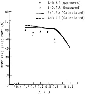
Otsuka et al. expanded the theory of the absorption efficiency of the infinite rectenna array to that of the finite rectenna array and conducted WPT experiments to confirm the absorption efficiency of the rectenna array [OTS 90]. An experimental setup and image of the rectenna array are shown in Figure 2.23. The experimental results indicate that the absorption efficiency of the rectenna array can be approximately 100% (Figure 2.24). On the basis of these studies, it can be considered that the BE can be almost 100% with τ > 2 in the WPT system via radiowaves.
Figure 2.23. Experimental setup of the investigation of the absorption efficiency of a rectenna array and an image of the rectenna array [OTS 90]
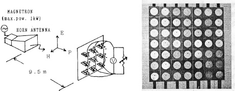
Figure 2.24. Element spacing (x-direction) and receiving efficiency of a rectenna array [OTS 90]