CHAPTER 5
FINITE ELEMENT FORMULATION: LARGE-DEFORMATION, LARGE-ROTATION PROBLEM
In the preceding chapters, the general nonlinear continuum mechanics theory was presented. In order to make use of this theory in many practical applications, a finite dimensional model must be developed. In this model, the partial differential equations of equilibrium are written using approximation methods as a finite set of ordinary differential equations. One of the most popular approximation methods that can be used to achieve this goal is the finite element method. In this method, the spatial domain of the body is divided into small regions called elements. Each element has a set of nodes, called nodal points, that are used to connect this element with other elements used in the discretization of the body. The displacement of the material points of an element is approximated using a set of shape functions and the displacements of the nodes and possibly their derivatives with respect to the spatial coordinates. In this case, the dimension of the problem depends on the number of nodes and number and type of the nodal coordinates used.
Small- and Large-Deformation Problems
In the literature, there are many finite element formulations that are developed for the deformation analysis of mechanical, aerospace, structural, and biological systems. Some of these formulations are developed for small-deformation and small-rotation linear problems, some for large-deformation and large-rotation nonlinear analysis, and the others for large-rotation and small-deformation nonlinear problems. Several numerical solution procedures and computational algorithms are also proposed for solving the resulting system of finite element differential equations.
The following chapter is devoted to the important nonlinear problem of small deformation and large rotation of flexible bodies, which is typical of multibody system (MBS) applications. In the case of small deformations, one can use more efficient formulations that employ smaller number of coordinates. These formulations, as will be discussed in the following chapter, allow for filtering out complex deformation shapes associated with high-frequency modes of oscillations while ensuring correct description of arbitrary rigid-body displacements. To this end, the concept of the intermediate element coordinate system will be introduced. The treatment of the more general problem of large deformation and large rotation, on the other hand, does not allow for such an efficient use of the techniques of coordinate reduction because the shape of deformations can be very complex and higher-order models are required in order to be able to capture the details of the deformation shapes. Nonetheless, in many large-deformation applications, one deals with softer materials that do not exhibit high-frequency oscillations, and for this reason, large-deformation formulations can be efficiently used.
Absolute Nodal Coordinate Formulation (ANCF)
In this chapter, a more general large-rotation and large-deformation finite element formulation is discussed. This formulation, which is called the absolute nodal coordinate formulation (ANCF), imposes no restrictions on the amount of rotation or deformation within the finite element. In addition to its simplicity and its consistency with the nonlinear theory of continuum mechanics, the absolute nodal coordinate formulation has several advantages as compared to other large-rotation and large-deformation finite element formulations that exist in the literature. This formulation leads to a constant mass matrix and zero centrifugal and Coriolis forces; allows for the use of general constitutive models in case of beams, plates, and shells; and accounts for the dynamic coupling between the rigid-body motion and the elastic deformation.
There are three conditions that must be met in order to have the absolute nodal coordinate formulation discussed in this chapter. First, the problem under investigation must be a dynamic problem in order to address the formulation of the inertia forces. Second, consistent mass formulation must be used because lumped mass formulations do not lead to a correct representation of the rigid-body dynamics (Shabana, 2013). Third, global gradients or slopes obtained by differentiation of absolute position vectors with respect to the spatial coordinates are used as nodal coordinates in order to ensure continuity of rotation parameters. The latter requirement is particularly important when finite elements are assembled. In the assembly process, proper gradient transformation must be used instead of the vector transformation often used in the finite element literature. Gradients are tangent to coordinate lines, and therefore, for two gradient vectors to be equal they must be tangent to the same coordinate line. Understanding the concept of gradients is crucial in the ANCF implementation, particularly when discontinuities or initially curved structures are considered. Using ANCF finite elements one can develop a nonincremental solution procedure for solving large-deformation problems.
Chapter Organization
This chapter is organized as follows. In Section 1, the displacement field and coordinates of the finite element are defined. In Section 2, the element connectivity conditions are introduced. In Section 3, the finite element inertia and elastic forces are formulated, whereas in Section 4 the virtual work of the inertia and elastic forces of the element is used to formulate the virtual work expression of the equations of motion of the finite element. This virtual work expression is used to obtain the equations of motion of the deformable body by assembling the equations of its finite elements. Because ANCF finite elements leads to a nonlinear expression of the elastic forces, one must resort in general to evaluate numerically the integrals of these elastic forces, as discussed in Section 5. In Section 6, the basic differential geometry theories of curves and surfaces are briefly reviewed in order to help the reader better understand the modes of deformations of beams, plates, and shells. In Sections 7–13, several examples of two- and three-dimensional finite element shape functions are presented, and the procedures for formulating the elastic forces of these elements are outlined. In Section 14, the performance of the finite elements is discussed, including topics such as the patch test; shear, membrane, and volumetric locking; and reduced and selective integrations. In Section 15, other large-deformation finite element formulations used in the literature are discussed and compared with the ANCF presented in more detail in this chapter. The formulations of the dynamic equations obtained using the updated Lagrangian and Eulerian approaches are compared in Section 16.
5.1 DISPLACEMENT FIELD
In the finite element method, as previously pointed out, the domain of the body is divided into small regions called elements. Assuming that these elements are small, one can use low-order polynomials to describe the displacement field of the element. For example, if the deformation of the body is negligible or small, only six coordinates are sufficient to define the rigid-body translation and rotation. In this special case, first-order polynomials can be used to describe exactly the rigid-body motion. For a small finite element on a deformable body, on the other hand, the deformation within the element can be in general much smaller than the overall deformation of the body, and therefore, one can still justify using a lower-order polynomial to describe the displacement of a small region on the body. After introducing the low-order polynomials to define the equations of motion of the finite elements, the body equations of motion can be obtained by assembling the equations of motion of its elements using the connectivity conditions at the finite element boundaries. By using this procedure, one can develop a powerful tool for the computer-aided analysis of structural components that have complex geometric shapes.
Separation of Variables
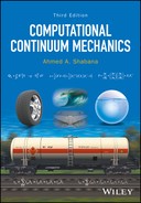
Finite element approximations are based on the concept of the separation of variables briefly introduced in Chapter 1 and used in the examples presented in several chapters of this book. The displacement of the finite element can be written as the product of two sets of functions: one set depends on the spatial coordinates, whereas the other set depends on time only. The separation of variables can conveniently be achieved by assuming that the position vector of arbitrary material points on the element can be written as polynomials of the spatial local coordinates of the element. The coefficients of these polynomials in the case of dynamics are the time-dependent variables. One can select points on the element, called nodes, and assign variables such as displacements, rotations, and slopes as nodal coordinates. Knowing the coordinates of these nodes in the reference configuration, one can write a set of algebraic equations using the assumed polynomial displacement field and determine the polynomial coefficients in terms of the nodal variables. In the formulation discussed in this section, all the components of the position vector are interpolated using polynomials that have the same order. For example, for a given domain defined by the spatial coordinates x1, x2, and x3, the kth component of the position vector can be written as
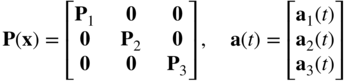
The coefficients aik, i = 0, 1, 2, 3, …, in the case of dynamics, are assumed to depend only on time. In this case, the above assumed displacement field can be written as the product of functions that depend only on the spatial coordinates x = [x1 x2 x3]T and a vector of time-dependent coordinates. To see this separation of variables, the preceding equation can be written as
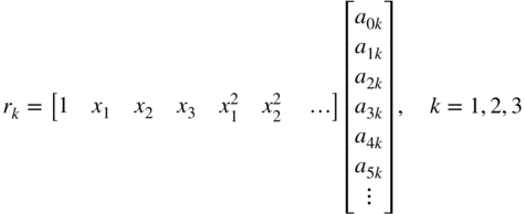
Denoting the space-dependent row in this equation as Pk(x) and the time-dependent vector as ak(t), the preceding equation can be written as
where
One can select, as discussed in Chapter 1 and demonstrated by the examples presented at the end of this section, position coordinates and possibly spatial derivatives of the coordinates at selected points and write the coefficients ak(t) in terms of these position coordinates and their derivatives. The number of the selected position coordinates and their derivatives must be equal to the number of the polynomial coefficients in order to have a number of algebraic equations, which can be solved for these coefficients. Let e be the vector of coordinates that may include position coordinates and their spatial derivatives at selected points at known local positions on the element. Substituting the values of the spatial coordinates in the preceding equation, one can write the following relationship between the selected coordinates and the coefficients of the polynomial:
where Bp is a constant square nonsingular matrix and a is the total vector of the polynomial coefficients. The preceding equation can be solved for the coefficients a in terms of the selected coordinates as ![]() . Substituting this equation into the assumed displacement field of Equation 3, one can write the displacement field in terms of the selected coordinates as
. Substituting this equation into the assumed displacement field of Equation 3, one can write the displacement field in terms of the selected coordinates as
In this equation,
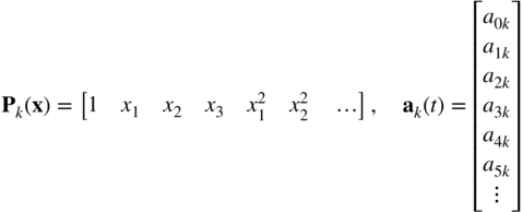
One, therefore, can write the position vector r using Equation 6 as
where ![]() . In this approach, S(x) is called the shape function matrix. The position vector field can then be written as the product of the space-dependent matrix S(x) and the vector of time-dependent coordinates e(t).
. In this approach, S(x) is called the shape function matrix. The position vector field can then be written as the product of the space-dependent matrix S(x) and the vector of time-dependent coordinates e(t).
Using this approach of the separation of variables, and assuming that the continuum is divided into a number of ne finite elements as shown in Figure 1, the displacement field of a finite element j can be written as
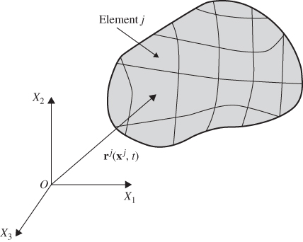
Figure 5.1 Finite element discretization
where rj is the global position vector of an arbitrary point on the finite element j as shown in Figure 1, Sj = Sj(xj) is a shape function matrix that depends on the element spatial coordinates ![]() defined in the element reference configuration, and ej = ej (t) is the vector of time-dependent nodal coordinates that define the displacements and possibly their spatial derivatives at a set of nodal points selected for the finite element.
defined in the element reference configuration, and ej = ej (t) is the vector of time-dependent nodal coordinates that define the displacements and possibly their spatial derivatives at a set of nodal points selected for the finite element.
Modes of Displacement
The selection of the number of nodal points and the number of coordinates at each node is one of the important factors that determine the accuracy of the finite element approximation. The general theory of continuum mechanics discussed in this book shows that the matrix of position vector gradients leads to nine independent modes of displacements for an infinitesimal volume at a material point. The polar decomposition theorem shows that the matrix of position vector gradients can be decomposed as the product of an orthogonal matrix and a symmetric matrix. The orthogonal matrix is function of three independent parameters that define the rotation of the infinitesimal volume, whereas the symmetric matrix is a function of six independent deformation parameters that define the strain components. Therefore, if the translation of the infinitesimal volume is considered, one has a total of 12 displacement modes for the infinitesimal volume: 3 translations, 3 rotations, and 6 deformation modes. Motivated by this simple and general continuum mechanics description of the motion of the infinitesimal volume, the vector of nodal coordinates can be selected in the three-dimensional analysis to consist of three translations and nine components of the position vector gradients. The nine components of the position vector gradients account for three rotations and six deformation modes. In this case, the vector of nodal coordinates ej of the finite element at a node k can be written as
where rjk is the absolute (global) position vector of the node k of the finite element j and ![]() is the vector of position gradients obtained by differentiation with respect to the spatial coordinate xl, l = 1, 2, 3. Note that
is the vector of position gradients obtained by differentiation with respect to the spatial coordinate xl, l = 1, 2, 3. Note that ![]() is the matrix of the position vector gradients at node k, where
is the matrix of the position vector gradients at node k, where ![]() . Note also that the last three vector elements of the vector of nodal coordinates ejk in Equation 10 are the columns of the matrix of position vector gradients
. Note also that the last three vector elements of the vector of nodal coordinates ejk in Equation 10 are the columns of the matrix of position vector gradients ![]() that enters in the formulation of the strain tensors. It is important that the chosen assumed displacement field and nodal coordinates correctly describe an arbitrary displacement including rigid-body displacement. This is an essential requirement, particularly in problems in the field of MBS dynamics in which the system components may undergo finite rotations.
that enters in the formulation of the strain tensors. It is important that the chosen assumed displacement field and nodal coordinates correctly describe an arbitrary displacement including rigid-body displacement. This is an essential requirement, particularly in problems in the field of MBS dynamics in which the system components may undergo finite rotations.
Nodal Coordinates
In the finite element literature, one can find a large number of finite elements that have been developed to suit varieties of applications. Some elements take the shape of trusses, some the shape of beams, some the shape of rectangle, triangle or plate, solid (prism), tetrahedral, and many other shapes. These elements employ different numbers and types of nodal coordinates. For example, solid, triangle, rectangle, and tetrahedral elements employ, for the most part, only displacement coordinates. Rotations, slopes, or gradients are not commonly used for these elements. Conventional beam, plate, and shell elements employ, in addition to the displacement coordinates, infinitesimal rotation coordinates. Arbitrary rigid body motion, however, cannot be defined as linear functions of infinitesimal rotations. Some newer beam, plate, and shell elements use finite rotations as nodal coordinates and define a rotation field that is independent from the displacement field. Because in the general theory of continuum mechanics, the rotation field is defined from the displacement field using the matrix of position vector gradients, the use of an independent finite rotation field can lead to coordinate redundancy, which can be a source of fundamental and numerical problem (Ding et al., 2014). Discussion on other types of finite elements and finite element formulations is presented in a later section.
In the ANCF discussed in this chapter, no infinitesimal or finite rotations are used as nodal coordinates. In this formulation, only absolute position vectors consistent with the general continuum mechanics are interpolated, and the position vector gradient field is obtained by differentiation of the position vector field with respect to the spatial coordinates of the finite element. As will be shown in this chapter, in addition to having a description consistent with the general continuum mechanics theory, the formulation discussed in this chapter has many unique features that make it suited for the analysis of large deformation and large rotation of very flexible structures.
5.2 ELEMENT CONNECTIVITY
In order to obtain the equations of motion of the continuum, the finite elements that form the continuum domain must be properly connected at the nodal points. Let the vector of nodal coordinates of all elements before connecting them be denoted as eb. This vector is then given by
where ej is the vector of nodal coordinates of the finite element j and ne is the total number of finite elements. Let e be the vector of all nodal coordinates of the continuum after the elements are connected. It is assumed that the finite element coordinates are defined in the same coordinate system as the continuum coordinates. The case in which the element nodal coordinates are defined in a coordinate system different from the continuum reference coordinate system will be also discussed. The vector of the element j coordinates can be written in terms of the nodal coordinates of the body as
where Bj is a Boolean matrix that includes zeros and ones and maps the element coordinates to the body coordinates. If the finite elements have different orientations, which is the case of slope discontinuity, a constant transformation can be defined and can be systematically introduced into the preceding equation (Shabana and Mikkola, 2003; Shabana, 2011). In this case, one can first define the element coordinates by the vector ēj and write this vector in terms of element nodal coordinates defined in the same coordinate system as the continuum (body) nodal coordinates, that is, ēj = Tjej, where Tj is an element transformation matrix (Shabana and Mikkola, 2003; Shabana, 2011) and ej is a vector of nodal coordinates defined in the same coordinate system as the body nodal coordinates. The Boolean matrix Bj can then be used to write the vector of the element nodal coordinates in terms of the body nodal coordinates as ēj = TjBje. In the case of using position vector gradients as nodal coordinates, a proper transformation for the gradients must be used. In the remainder of this chapter, for simplicity, we will assume that such a transformation is applied and use Equation 12 with the understanding that the element and the body nodal coordinates ej and e are properly defined in the same coordinate system.
Using Equation 12, one can then write
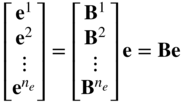
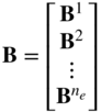
where B is the Boolean matrix formed using the element Boolean matrices as
This matrix has a number of rows equal to the dimension of the vector eb and a number of columns equal to the dimension of the vector e. This procedure of assembling the finite elements is demonstrated by the following simple example.
5.3 INERTIA AND ELASTIC FORCES
In this section, the formulation of the finite element inertia and elastic forces is discussed. It will be shown that the finite element formulation discussed in this chapter leads to a simple expression for the inertia forces and to a more complex expression for the elastic forces. This is in contrast with the floating frame of reference (FFR) formulation discussed in the following chapter and used mainly for the small-deformation, large-rotation analysis. The FFR formulation leads to a complex expression for the inertia forces and to a simple expression for the elastic forces.
Inertia Forces
In order to formulate the inertia forces of the finite element, one must obtain an expression for the acceleration vector. Differentiating the global position vector of Equation 9 with respect to time, the absolute velocity vector vj of an arbitrary material point on the element j can be written as
Differentiating this equation with respect to time, the acceleration vector aj can be written in the case of the ANCF as
The virtual work of the inertia forces of the finite element can then be defined as
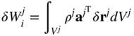
where ρj and Vj are, respectively, the mass density and volume of the finite element. It is important to point out that because of the principle of conservation of mass, ρjdVj = constant, the mass density ρj, and the volume Vj in the reference configuration can be used. For the simplicity of the notation in this chapter, we use ρj instead of ![]() to denote the density in the reference configuration because in most of the developments presented in this chapter and the following one, the inertia can be formulated using the reference configuration. A specific mention will be made if ρj is the mass density associated with the current configuration, as it is the case when the equations that govern the fluid motion are discussed.
to denote the density in the reference configuration because in most of the developments presented in this chapter and the following one, the inertia can be formulated using the reference configuration. A specific mention will be made if ρj is the mass density associated with the current configuration, as it is the case when the equations that govern the fluid motion are discussed.
The virtual change in the position vector of the material point can be written as
Using the preceding two equations with the expression for the acceleration of Equation 16 and keeping in mind that the time-dependent nodal coordinates do not depend on the spatial coordinates and can be factored out of the integration sign, one obtains the following equation for the virtual work of the inertia forces:
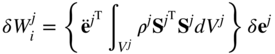
This equation can be written as
where Mj is the symmetric mass matrix of the finite element j defined as
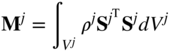
This mass matrix is constant in both two- and three-dimensional cases. This is a unique feature of the ANCF because other known three-dimensional finite element formulations that give complete information about the rotation at the nodes and use infinitesimal or finite rotation parameters as nodal coordinates do not lead to a constant mass matrix in the case of three-dimensional analysis. This important property of the formulation simplifies the governing equations significantly since it leads to zero centrifugal and Coriolis forces when the body experiences an arbitrary large deformation and finite rotation.
By using the preceding equations, the virtual work of the inertia forces can be written as
where ![]() is the vector of the inertia forces that takes the following simple form:
is the vector of the inertia forces that takes the following simple form:
One can show that, for many ANCF finite elements, the mass matrix remains the same under an orthogonal coordinate transformation.
Elastic Forces
An expression for the virtual work of the stresses of the continuum was obtained in Chapter 3 in terms of the Green–Lagrange strain tensor and the second Piola–Kirchhoff stress tensor. For the finite element j, the virtual work of the stresses can be written as
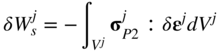
In this equation, ![]() is the second Piola–Kirchhof stress tensor and ϵj is the Green–Lagrange strain tensor at an arbitrary material point on the finite element j. The stress and strain tensors used in Equation 24 are defined in the reference configuration. The virtual strain can be expressed in terms of the virtual changes of the position vector gradients as
is the second Piola–Kirchhof stress tensor and ϵj is the Green–Lagrange strain tensor at an arbitrary material point on the finite element j. The stress and strain tensors used in Equation 24 are defined in the reference configuration. The virtual strain can be expressed in terms of the virtual changes of the position vector gradients as
The second Piola–Kirchhoff stresses are related to the Green–Lagrange strains using the constitutive equations
where Ej is the fourth-order tensor of elastic coefficients. Substituting the preceding two equations into the expression of the virtual work of the stresses, using the definition of the matrix of position vector gradients, and using the expression of the gradients in terms of the finite element nodal coordinates, one can show that the virtual work of the stresses of the finite element j can be written as
In this equation, ![]() is the vector of the elastic forces associated with the nodal coordinates of the finite element j. This vector, which is the result of the deformation of the continuum, takes a more complex form as compared to the simple expression of the inertia forces obtained previously in this section. Because the integrals for the stress forces are, in general, highly nonlinear functions in the nodal and spatial coordinates, numerical integration methods are often used for the evaluation of the nonlinear generalized stress forces.
is the vector of the elastic forces associated with the nodal coordinates of the finite element j. This vector, which is the result of the deformation of the continuum, takes a more complex form as compared to the simple expression of the inertia forces obtained previously in this section. Because the integrals for the stress forces are, in general, highly nonlinear functions in the nodal and spatial coordinates, numerical integration methods are often used for the evaluation of the nonlinear generalized stress forces.
5.4 EQUATIONS OF MOTION
The equations of motion of the finite elements that form the body can be developed using the principle of virtual work in dynamics (Roberson and Schwertassek, 1988; Shabana, 2001). In the case of unconstrained motion, the principle of virtual work for the continuum can be written as
In this equation, δWi is the virtual work of the inertia forces of the body, δWs is the virtual work of the elastic forces due to the deformation, and δWe is the virtual work of the applied forces such as gravity, magnetic, and other external forces. For instance, the virtual work of an external force Fj acting at a point P defined by the coordinates ![]() on the finite element j can be written as
on the finite element j can be written as
where ![]() is a constant matrix that defines the element shape function at point
is a constant matrix that defines the element shape function at point ![]() and
and ![]() is the vector of generalized forces associated with the element nodal coordinates ej as the result of the application of the force vector Fj. This vector of generalized forces is defined as
is the vector of generalized forces associated with the element nodal coordinates ej as the result of the application of the force vector Fj. This vector of generalized forces is defined as
A similar expression can be obtained for all forces acting on the finite elements. One can then write the virtual work of the applied forces acting on the continuum by summing up the virtual work of the forces acting on its finite elements, that is,
The virtual work of the inertia forces of the body can be obtained by summing up the virtual work of the inertia forces of its finite elements. Using the expression of the virtual work of the finite element inertia forces obtained in the preceding section, one can write
Similarly, the virtual work of the stress forces of the body can be written as
Substituting the preceding three equations into the principle of virtual work in dynamics of Equation 28, one obtains
This equation can also be written as
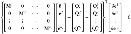
Because δej = Bjδe and ëj = Bjë, where Bj is a Boolean matrix that defines the element connectivity and e is the vector of the body nodal coordinates, Equation 34 can be written in terms of the nodal coordinates of the body as
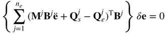
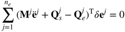
If the body motion is unconstrained, the elements of the vector δe are independent, and as a consequence, their coefficients in the preceding equation must be equal to zero, that is,
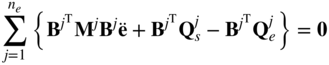
By performing the summation in this equation, one can show that the finite element equation of motion of the body can be written as
where M is the body symmetric mass matrix, Qs is the vector of body elastic forces, and Qe is the vector of the body applied forces. The mass matrix and force vectors that appear in the preceding equation are obtained from the mass matrices and force vectors of the finite elements as
In the finite element formulation discussed in this chapter, the body mass matrix is constant, and therefore, the vectors of centrifugal and Coriolis forces are identically equal to zero in this formulation. The vector of the body elastic forces due to the stresses, on the other hand, is a nonlinear function of the nodal coordinates, as discussed in the preceding section. The fact that the mass matrix is constant can be utilized in developing a computational algorithm for solving the finite element equations. In this case, there is no need to iteratively perform the LU factorization of this matrix. One can use a transformation based on Cholesky coordinates that leads to an identity mass matrix (Shabana, 1998). Such a coordinate transformation leads to an optimum sparse matrix structure when ANCF finite elements are used in MBS algorithms.
Curved Geometry
ANCF finite elements can be used to conveniently describe complex shapes. These shapes can represent curved geometry in the undeformed reference configurations. In these cases, the position vector gradients in the undeformed reference configuration are not orthogonal unit vectors because of the continuum initial geometry. Examples of these applications, which were presented in Chapter 2 and include tires, belt drives, and tank cars, are shown in Figure 4. As discussed in Chapter 2, in these cases, the strains evaluated using the matrix of position vector gradients in the initial configuration must be identically equal to zero. In order to explain how the strains are formulated in these cases of initial curved geometry, the three different configurations shown in Figure 5 were considered in Chapter 2. Because complex geometries can always be obtained by changing the shape of simple objects, the first configuration in Figure 5 depicts the simple geometry, which can represent straight metal sheets described conveniently using ANCF finite elements. In this simple geometry configuration, the location of the material points is defined using the position vector ![]() of the ANCF element or an assembly of ANCF finite elements. The second configuration is the reference configuration, which defines the initial undeformed geometry. In this undeformed reference configuration, the position of the material points is defined by the vector
of the ANCF element or an assembly of ANCF finite elements. The second configuration is the reference configuration, which defines the initial undeformed geometry. In this undeformed reference configuration, the position of the material points is defined by the vector ![]() . One can write
. One can write ![]() , where
, where ![]() , and the superscript that indicates the finite element number is dropped for simplicity. The third configuration shown in Figure 5 defines the current deformed configuration. In this configuration, the position of the material points is defined by the vector
, and the superscript that indicates the finite element number is dropped for simplicity. The third configuration shown in Figure 5 defines the current deformed configuration. In this configuration, the position of the material points is defined by the vector ![]() . As discussed in Chapter 2, one can write
. As discussed in Chapter 2, one can write ![]() , with
, with ![]() . It follows that
. It follows that ![]() , where
, where ![]() .
.
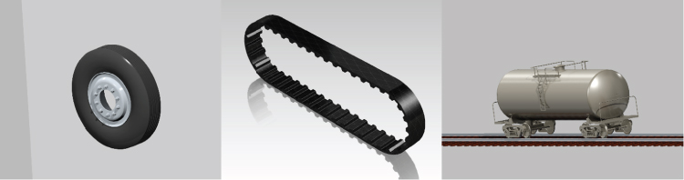
Figure 5.4 Initial geometry
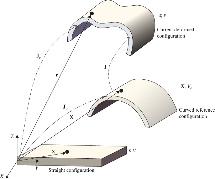
Figure 5.5 ANCF description of curved geometry
The volume of the curved structure ![]() is related to the volume of the straight structure
is related to the volume of the straight structure ![]() (Figure 5) using the relationship
(Figure 5) using the relationship ![]() , where
, where ![]() is the determinant of the matrix of position vector gradients
is the determinant of the matrix of position vector gradients ![]() . Therefore, integration with respect to the domain
. Therefore, integration with respect to the domain ![]() can be converted to integration with respect to the straight domain
can be converted to integration with respect to the straight domain ![]() by using the transformation
by using the transformation ![]() . This allows for using the original dimensions of the simpler geometry to carry out the integrations associated with the initially curved configuration. Note that the matrix
. This allows for using the original dimensions of the simpler geometry to carry out the integrations associated with the initially curved configuration. Note that the matrix ![]() is constant.
is constant.
The matrix of position vector gradients ![]() is the matrix, which is used to determine the Lagrangian strain tensor
is the matrix, which is used to determine the Lagrangian strain tensor ![]() as
as ![]() . This matrix can be defined using the ANCF description as
. This matrix can be defined using the ANCF description as
where, as previously defined, ![]() . Therefore, the Lagrangian strain tensor can be written as
. Therefore, the Lagrangian strain tensor can be written as
Note that the relationship between the volume in the current deformed configuration ![]() and the volume in the curved reference configuration
and the volume in the curved reference configuration ![]() can be written as
can be written as ![]() , where
, where ![]() is the determinant of the matrix of position gradients
is the determinant of the matrix of position gradients ![]() . It follows that
. It follows that ![]() . Using the relationship
. Using the relationship ![]() , one has
, one has ![]() .
.
As mentioned in Chapter 2, the procedure described in this section to model the initial curvature, which is the same as the one used in the literature for modeling the initially curved configuration of belt drives and rubber chains (Dufva et al., 2007; Maqueda et al., 2010), will lead to zero strains for an arbitrary initially curved geometry. Using the ANCF finite elements discussed later in this chapter, the constant matrix of position vector gradients ![]() can be determined in a straightforward manner. In the ANCF description, the assumed displacement field can be written as
can be determined in a straightforward manner. In the ANCF description, the assumed displacement field can be written as ![]() , where
, where ![]() is the global position vector,
is the global position vector, ![]() is the vector of the element spatial coordinates,
is the vector of the element spatial coordinates, ![]() is time,
is time, ![]() is the element shape function matrix, and
is the element shape function matrix, and ![]() is the vector of the element nodal coordinates that include absolute position and gradient coordinates. In the ANCF description, the vector of nodal coordinates
is the vector of the element nodal coordinates that include absolute position and gradient coordinates. In the ANCF description, the vector of nodal coordinates ![]() can be written as
can be written as ![]() , where
, where ![]() is the vector of nodal coordinates in the reference configuration and
is the vector of nodal coordinates in the reference configuration and ![]() is the vector of nodal displacements. Using this partitioning, the assumed displacement field can be written as
is the vector of nodal displacements. Using this partitioning, the assumed displacement field can be written as ![]() . Using the general continuum mechanics description
. Using the general continuum mechanics description ![]() , where
, where ![]() is the absolute position vector of an arbitrary point in the reference configuration and
is the absolute position vector of an arbitrary point in the reference configuration and ![]() is the displacement vector, one can write
is the displacement vector, one can write ![]() and
and ![]() . By appropriate choice of the elements of the vector
. By appropriate choice of the elements of the vector ![]() , initially curved structures can be defined in a straightforward manner using ANCF finite elements.
, initially curved structures can be defined in a straightforward manner using ANCF finite elements.
As previously mentioned, integration with respect to the domain ![]() can be converted to integration with respect to the straight element domain
can be converted to integration with respect to the straight element domain ![]() by using the transformation
by using the transformation ![]() , where
, where ![]() is the determinant of the matrix of position vector gradients
is the determinant of the matrix of position vector gradients ![]() . In the ANCF description, the matrix
. In the ANCF description, the matrix ![]() is constant, while
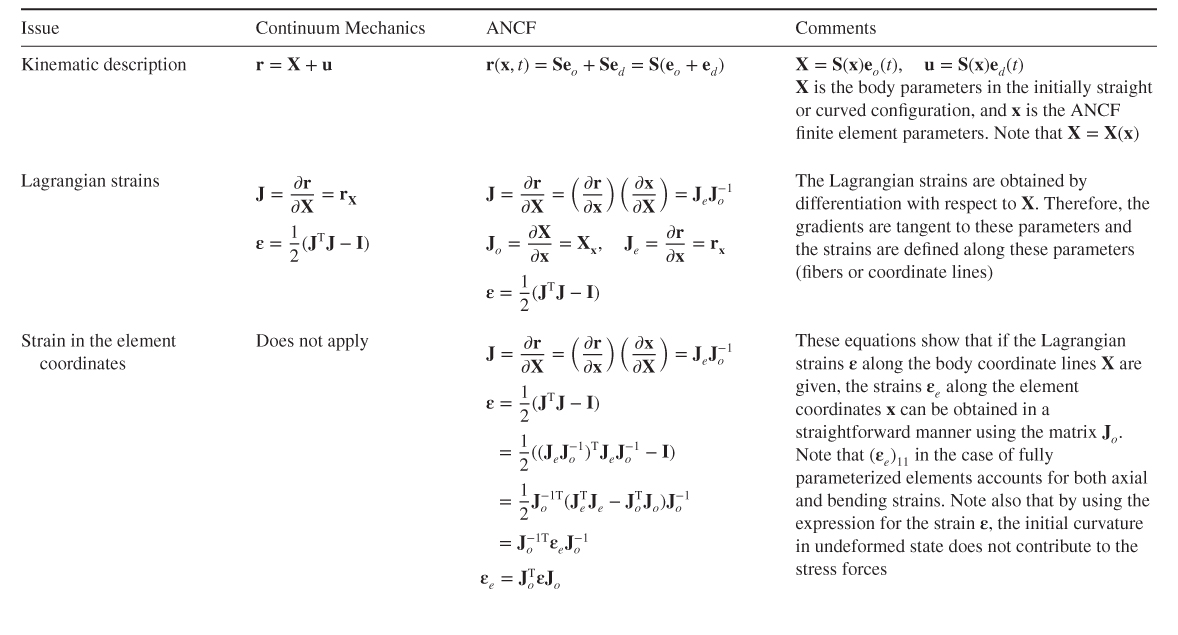
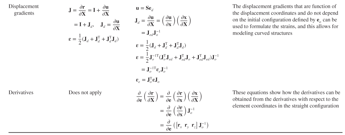
is constant, while ![]() . Table 1 explains how the basic continuum mechanics description is implemented using ANCF finite elements.
. Table 1 explains how the basic continuum mechanics description is implemented using ANCF finite elements.
Table 5.1 ANCF Description of Curved Geometry
5.5 NUMERICAL EVALUATION OF THE ELASTIC FORCES
As previously pointed out and shown in this chapter, the nonlinear large-deformation finite element absolute nodal coordinate formulation leads to a simple expression for the inertia forces and a nonlinear expression for the stress elastic forces. This is in contrast with the small-deformation finite element FFR formulation presented in the following chapter. The FFR formulation leads to a simple expression for the elastic forces and to a highly nonlinear expression for the inertia forces. Nonetheless, as will be shown in the following chapter, the nonlinear inertia forces obtained using the FFR formulation can be expressed in terms of a unique set of inertia shape integrals. These shape integrals can be evaluated in advance of the dynamic simulation using information from existing structural dynamics finite element codes.
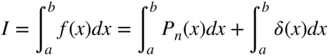
Because closed-form expressions for the nonlinear ANCF elastic forces cannot be, in general, obtained, the numerical evaluation of these forces is discussed in this section. The numerical evaluation of integrals of functions is covered in detail in textbooks on numerical methods (Carnahan et al., 1969; Atkinson, 1978). Therefore, in this section, a brief introduction to this subject is presented. To this end, consider the following integral of a single function f(x) over the interval [a, b]:
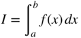
If the function f(x) is not simple or is given in a tabulated form, analytical evaluation of the preceding integral can be difficult, or even impossible. In these cases, one must resort to numerical methods in order to evaluate the integral. Formulas used for numerical integration are called quadratures. One approach is to try to find a polynomial Pn(x) of order n that can be a good approximation of f(x). One can then obtain the integral of the polynomial in a closed form. Because Pn(x) is not in general the same as f(x), one can define the following error function:
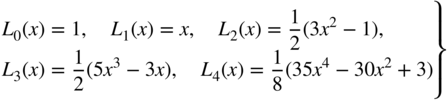
In general, δ(x) can take positive and negative values, and as a consequence, some of the positive errors cancel the effect of the negative errors when the integral ![]() is evaluated even in the case when Pn(x) is not a good approximation of f(x). For this reason, integration is known as a smoothing process (Carnahan et al., 1969). Furthermore, if f(x) is a polynomial or a function, which is described by data representing a polynomial, then one can always find a polynomial Pn(x) such that the integral I is exact. If f(x) is not a polynomial, the numerical integration will give an approximate evaluation of the integral of f(x). If the functions used in the approximation of the integrals are evaluated at equally spaced base points, one obtains the Newton–Cotes formulas, an example of which is the well-known Simpson's rule for numerical integration. If the functions used to approximate the integrals are evaluated using unequally spaced base points, one obtains the Gauss quadrature formulas. In the Gauss quadrature formulas, the locations of the base points are selected to achieve the best accuracy. In these formulas, the properties of orthogonal polynomials are used. Examples of orthogonal polynomials are the Legendre, Laquerre, Chebyshev, and Hermite polynomials. For example, the first few Legendre polynomials are defined as (Carnahan et al., 1969)
is evaluated even in the case when Pn(x) is not a good approximation of f(x). For this reason, integration is known as a smoothing process (Carnahan et al., 1969). Furthermore, if f(x) is a polynomial or a function, which is described by data representing a polynomial, then one can always find a polynomial Pn(x) such that the integral I is exact. If f(x) is not a polynomial, the numerical integration will give an approximate evaluation of the integral of f(x). If the functions used in the approximation of the integrals are evaluated at equally spaced base points, one obtains the Newton–Cotes formulas, an example of which is the well-known Simpson's rule for numerical integration. If the functions used to approximate the integrals are evaluated using unequally spaced base points, one obtains the Gauss quadrature formulas. In the Gauss quadrature formulas, the locations of the base points are selected to achieve the best accuracy. In these formulas, the properties of orthogonal polynomials are used. Examples of orthogonal polynomials are the Legendre, Laquerre, Chebyshev, and Hermite polynomials. For example, the first few Legendre polynomials are defined as (Carnahan et al., 1969)
In general, the Legendre polynomials are defined by the following general recursion relation:
One can show that these polynomials are orthogonal on the interval [−1, 1]. That is,
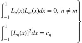
Because the Legendre polynomials are orthogonal, an arbitrary polynomial can be described as a linear combination of the Legendre polynomials.
Gaussian Quadrature
In the Gaussian quadrature formulas, the integral is evaluated by approximating the function f(x) by a polynomial Pn(x) defined at unequally spaced base points. This function approximation can lead to an error δ(x), as previously mentioned. The locations of the base points are determined by developing a set of algebraic equations that make the integral of the error function equal to zero. The solution of these algebraic equations, which are obtained using the properties of the orthogonal polynomials, defines the base points. One can then write the integral I in the following form:
The domain of integration can be changed from x ∈ [a, b] to ξ ∈ [−1, 1] by using the substitution
The steps used to determine the base points are first to employ the Lagrangian interpolating polynomials to approximate Pn(x) and δ(x). The Lagrangian interpolating polynomials do not require equally spaced base points. The resulting polynomials are then expressed in terms of the orthogonal Legendre polynomials. The Legendre polynomial orthogonality conditions are used to define a set of algebraic equations that make the integral of the error function equal to zero. This set of algebraic equations defines the base points for different orders of the polynomial Pn(x). The integral can then be written in terms of the function evaluated at these base points multiplied by weight factors or weight coefficients. This procedure for determining the base points is described in detail by Carnahan et al. (1969). The results are weight factors, which depend on the order of the polynomial or the number of base points selected to approximate f(x). These weight factors are presented in tables in mathematics handbooks or in textbooks on the subject of numerical analysis. In general, if the integral of the error function becomes zero and the domain of integration is changed to [−1, 1], the integral I can be written in terms of the function at the base points and the weight coefficients as
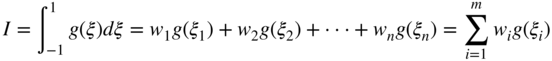
where wi, i = 1, 2, …, m, are the weight factors. These weight factors are called Gauss–Legendre coefficients. The weight factors are selected in order to achieve the greatest accuracy. Symmetrically located base points have the same weight coefficients. Note that if g(ξ) is approximated by one quadrature point, there is only one base point ξ1 = 0. In this case, the integral is given by ![]() . If g(ξ) is an arbitrary linear function (n = 1), this integration result obtained using one quadrature point is exact. In this case, w1 represents the length of the domain of integration, that is, w1 = 2, and g(ξ1) is the height used to determine the area under the curve. In this case, the function g(ξ) is evaluated at ξ1 = 0, which represents the center of the interval. If g(ξ), on the other hand, represents a higher-order function, the one-point quadrature integration is an approximation. In general, a polynomial of degree n requires m = (n + 1)/2 quadrature base points for exact integration, where in this simple rule n is assumed an odd number.
. If g(ξ) is an arbitrary linear function (n = 1), this integration result obtained using one quadrature point is exact. In this case, w1 represents the length of the domain of integration, that is, w1 = 2, and g(ξ1) is the height used to determine the area under the curve. In this case, the function g(ξ) is evaluated at ξ1 = 0, which represents the center of the interval. If g(ξ), on the other hand, represents a higher-order function, the one-point quadrature integration is an approximation. In general, a polynomial of degree n requires m = (n + 1)/2 quadrature base points for exact integration, where in this simple rule n is assumed an odd number.
Generalization
The procedure used for integrating a function that depends on one variable can be generalized to the case in which the function depends on two or three variables, as it is the case in some finite element assumed displacement fields. In the two-dimensional case, consider the function g(ξ, η). It is assumed that the domains of integration are changed as discussed before such that ξ ∈ [−1, 1], and η ∈ [−1, 1]. The integral of the function g(ξ, η) can then be written as
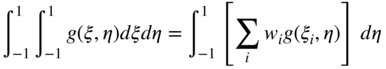
Performing the second integration with respect to η, one obtains
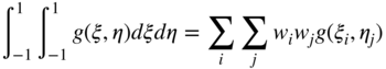
Following a similar procedure, one can show that in the case of a function that depends on three variables, ξ, η, and ζ, one has the following Gauss quadrature formula:
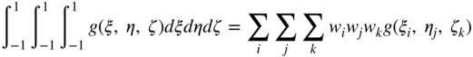
If the original function is expressed in terms of the coordinates x1, x2, and x3, that is, f = f(x1, x2, x3), the preceding formula requires using the relationship dx1dx2dx3 = Jdξdηdζ, where J is the determinant of the Jacobian of the coordinate transformation.
Using the Gauss quadrature formulas presented in this section, a systematic procedure for the numerical evaluation of the nonlinear stress elastic forces of the finite elements can be developed. The number of quadrature points used in the numerical integration defines the accuracy of the integration, and therefore, this number must be carefully selected in order to avoid increasing the computational cost or obtaining inaccurate results. There is no advantage gained from using a number of quadrature points larger than the number that gives exact evaluation of the integral (full integration). In some applications, on the other hand, there is an advantage in selecting a number of points that does not yield exact evaluation of the integrals. This is the case of reduced integration, which is commonly adopted in the finite element computational algorithms and will be discussed in a later section.
5.6 FINITE ELEMENTS AND GEOMETRY
In the following sections, examples of several finite elements that can be used to study the large deformations in a wide range of applications are presented. These elements have been developed over the last few years, and more details on the formulation of their shape functions, the mass matrices, and the vectors of elastic forces can be found in the literature. Some of these elements have been already used in this book in the examples presented in this chapter and preceding chapters.
General Continuum Mechanics Approach and Classical Theories
It is important to point out that in all the finite elements that are discussed in this chapter, classical theories can be used by introducing a local element frame. Therefore, for beam elements, one can still use Euler–Bernoulli and Timoshenko beam theories; and, for plate and shell elements, one can still use Kirchhoff and Mindlin plate theories. This can always be accomplished by using the element local frame, which serves the only purpose of measuring the deformation (Shabana, 2013), and such a frame does not enter into the formulation of the inertia forces. Therefore, it is important to distinguish between this local element frame and the corotational frame used in the finite element literature. If the general continuum mechanics approach is used instead of the classical theories, one obtains more general formulations that relax the assumptions of Euler–Bernoulli, Timoshenko, Kirchhoff, and Mindlin theories. In these general formulations, the element cross section is allowed to deform.
Gradient Vectors
Some of the elements presented in this chapter employ a complete set of gradient vectors as nodal coordinates. These elements allow, in a straightforward manner, for the use of a general continuum mechanics approach to formulate the elastic forces. The use of these elements also allows for using more general constitutive relationships. Elements that do not employ a complete set of parameters required to evaluate all the gradient vectors are called in this book, gradient deficient. The use of a general continuum mechanics approach with these elements is not as straightforward as compared to elements that have a complete set of parameters (spatial coordinates). The latter elements are called fully parameterized elements.
Locking Problems
ANCF finite elements were introduced to deal with very flexible components. These finite elements perform well in the case of very flexible bodies, and efficient solutions for large deformations of very flexible bodies can be obtained because a nonincremental solution procedure can be used with these ANCF elements. As the element stiffness decreases, ANCF elements become more efficient. Some researchers, however, used ANCF finite elements in the analysis of thin and stiff structures. In this case, some elements exhibit locking problems when the general continuum mechanics approach is used to formulate the elastic forces. The general continuum mechanics approach leads to what is called ANCF-coupled deformation modes (Hussein et al., 2007). These modes, which couple the deformation of the cross section and other deformations such as bending, can have high frequencies and can be a source of numerical problems (Schwab and Meijaard, 2005). Several techniques were proposed in the literature to solve the locking problems and improve the element performance.
In order to better understand the behavior of the finite elements introduced in the following sections, an understanding of the geometry is necessary. Some basic results from the theories of curves and surfaces, which are covered in the subject of differential geometry, can help the reader better understand and solve the problems encountered when ANCF finite elements are used.
Theory of Curves
The centerline of a beam element represents a space curve. A curve can be uniquely defined in terms of one parameter. That is, the Cartesian coordinates that define the curve can be determined once this parameter is specified. Let α be the parameter that defines the curve over the interval a ≤ α ≤ b. The curve can then be represented by the following parametric form:
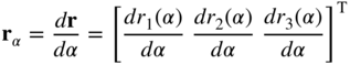
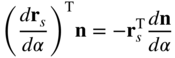
The tangent vector to the curve at α is given by
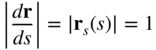
If at a given point α, |dr(α)/dα| = 0, the point is called a singular point. The parameter α can be selected to be the arc length s. If the arc length is used as a parameter, the tangent vector rs is a unit vector. That is,
In order to mathematically prove this important result, let r be the vector that defines the position of the points on a space curve. One can write the following equation:
If Δα is assumed small, Δr defines the tangent vector. In this case, if s is assumed to be the arc length of the space curve that defines the centerline of the element, then one has
This equation shows that in the limit when Δs approaches zero, one has
That is, the tangent vector obtained by differentiation with respect to the arc length is indeed a unit vector.
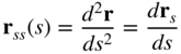
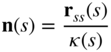
If a curve is parameterized by its arc length, the derivative of the unit tangent vector defines the curvature vector. That is, the curvature vector is defined as
The magnitude of the curvature vector at a given s is called the curvature and given as
Because the tangent vector rs(s) is a unit vector, the curvature κ(s) measures the rate of change of orientation of the tangent vector, that is, it measures the amount of bending of the curve. The preceding two equations show that linear displacement fields lead to zero curvature and, therefore, such fields are not appropriate for describing the displacement of components subjected to bending. Although one can approximate a curve by a large number of straight segments, in the finite element implementation the use of linear field will require the use of a very large number of finite elements. This increases the dimensions of the problem and can lead to a very inefficient solution procedure.
Because the tangent and curvature vectors are orthogonal, a unit vector along the curvature vector defines the unit normal to the curve n given as
The unit tangent and normal vectors form a plane called the osculating plane. The radius of curvature of the curve at s is defined as R = 1/κ(s). A vector normal to the osculating plane, called the binomial vector at s, is given by
The three orthogonal unit vectors rs, n, and b form a coordinate system called the Frenet frame.
Differentiating Equation 62 with respect to s and keeping in mind that the vectors rss(s) and n(s) are parallel, one obtains
This equation shows that bs(s) is normal to rs. Furthermore, because b(s) is a unit vector, bs(s) and b(s) are two orthogonal vectors, and bs(s) is parallel to n. Therefore, bs(s) can be written in the following form:
where τ is called the torsion. The curvature and torsion uniquely define the space curve.
Theory of Surfaces
Whereas a general space curve can be defined in terms of one parameter, a surface can be completely described in terms of two parameters s1 and s2. In general, a surface can be described in the following parametric form (Goetz, 1970; Kreyszig, 1991):
It is required that the mapping in this equation is one to one, and the Jacobian matrix
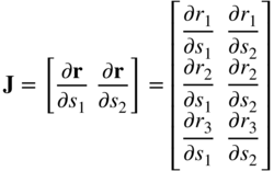
has a rank equal to two. This condition is satisfied if (∂r/∂s1) × (∂r/∂s2) ≠ 0, which implies that the two columns of the Jacobian matrix in the preceding equation are linearly independent. The two vectors ![]() and
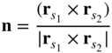
and ![]() represent the two tangent vectors at the point of intersection of the coordinate lines s1 and s2. The unit vector normal to the surface at this point can then be defined as
represent the two tangent vectors at the point of intersection of the coordinate lines s1 and s2. The unit vector normal to the surface at this point can then be defined as
As in the case of curves, the surface can be defined uniquely using local geometric quantities called the first and second fundamental forms. The first fundamental form of a surface is defined as follows:
This equation shows that the first fundamental form I can be used as a measure of distance or length. Using the fact that ![]() , the first fundamental form of the preceding equation can be written as
, the first fundamental form of the preceding equation can be written as
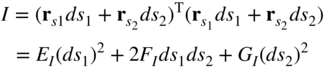
where
These coefficients are called the coefficients of the first fundamental form. One can show that distances, angles, and areas on the surface can be expressed in terms of the first fundamental form (Goetz, 1970; Kreyszig, 1991).
The second fundamental form of a surface is defined as
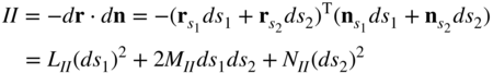
where n is the unit normal and the coefficients of the second fundamental form are defined as
Because ![]() and
and ![]() are perpendicular to n for all values of the parameters s1 and s2, one has the following identities:
are perpendicular to n for all values of the parameters s1 and s2, one has the following identities:
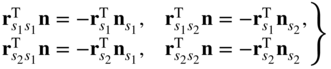
Using these identities, the coefficients of the second fundamental form can be written in an alternate form as follows:
where ![]() . Using the preceding equation, and the fact that
. Using the preceding equation, and the fact that
one can show that the second fundamental form can be written in the following alternate form:
This equation can be used to measure the rate of change of orientation of the tangent plane. The coefficients of the second fundamental form can be used to determine the nature of the surface in the neighborhood of an arbitrary point P. If ![]() , the surface is called elliptic. If
, the surface is called elliptic. If ![]() , the surface is called hyperbolic. If
, the surface is called hyperbolic. If ![]() , the surface is called parabolic. If LII = MII = NII = 0, the surface is called planar. Figure 6 shows examples of such surface geometry
, the surface is called parabolic. If LII = MII = NII = 0, the surface is called planar. Figure 6 shows examples of such surface geometry
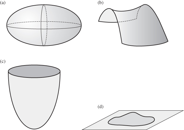
Figure 5.6 Surface geometry. (a) Elliptic surface, (b) hyperbolic surface, (c) parabolic surface, and (d) planar surface
Surface Curvature
One can always define a curve on a surface if the parameters s1 and s2 are expressed in terms of one parameter α. Let c = c(s1(α), s2(α)) be a regular curve defined on the surface r = r (s1, s2). The normal curvature vector to the curve c at point P denoted by Kn is defined as the projection of the curvature vector css of the curve onto the normal n to the surface at point P and is given by
In this equation, s is the arc length of the curve. Note that the curve c can be defined as the intersection of a plane that contains the tangent to c and the normal vector. The norm of the normal curvature vector defined in the preceding equation is called the normal curvature and is defined as
Recall that the curvature vector of the curve at a point P on the surface r is given by
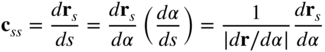
where rs is the tangent vector to the curve at P and s is the curve arc length. In deriving the preceding equation, one utilized the fact that |dr/dα| = |rs|(ds/dα) = (ds/dα), which is the consequence of the fact that |rs| = 1. Because rs is orthogonal to n, one has ![]() , which leads to
, which leads to
Substituting Equation 79 into Equation 78 and using Equation 80, one obtains
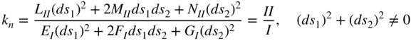
Because the first fundamental form I is positive, the sign of kn depends on the sign of the second fundamental form II. Using the preceding equation, one can show that kn = 0 in all directions for a planar point. For an elliptic point, kn ≠ 0 and has the same sign as the ratio ds1/ds2. In the case of a hyperbolic point, kn can be positive, negative, or zero, depending on the sign and value of ds1/ds2. For a parabolic point, kn maintains the same sign and it is zero if the second fundamental form II is equal to zero.
The directions that define the maximum or minimum values of the normal curvature can be obtained by differentiating Equation 81 with respect to the parameters s1 and s2, and setting the results equal to zero. That is,
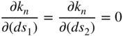
Substituting Equation 81 into these equations, one obtains
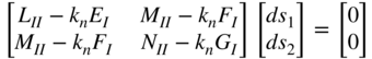
This equation has a nontrivial solution if and only if the determinant of the coefficient matrix is equal to zero, that is,
The solution of this quadratic equation defines two roots k1 and k2. These two roots, which are called the principal curvatures, can be substituted into Equation 83 to determine the principal directions. The mean curvature Km and the Gaussian curvature kG at a point P on the surface are defined in terms of the principal curvatures as
These surface definitions as well as the analysis of curve and surface geometry presented in this section are important to understand the behavior of beams, plates, and shells. Some of the obtained geometric results shed light on the order of approximation that must be used when employing the finite element method to solve beam, plate, and shell problems. For example, as previously discussed, the curvature is obtained from the second derivative of the position vector. Therefore, finite elements that employ linear or bilinear approximation cannot be effectively used in bending problems because the curvature will always be equal to zero. When these linear and bilinear elements are employed, one must use a very fine mesh in order to be able to represent a space curve or a shell by straight lines or flat sections, respectively. This approach tends to be very inefficient and, therefore, the use of structural finite elements that are based on higher-order interpolations is recommended. Some of these ANCF elements are discussed in the following sections.
5.7 TWO-DIMENSIONAL EULER–BERNOULLI BEAM ELEMENT
The Euler–Bernoulli beam element presented in this section has two nodes. Each node k for an element j has four coordinates; two translations rjk, and two gradient coordinates ![]() . Therefore, the vector of nodal coordinates has eight elements and is defined as
. Therefore, the vector of nodal coordinates has eight elements and is defined as
The shape function matrix of the element can be defined by using the following interpolation functions:
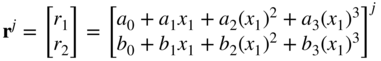
where ai and bi, i = 0, 1, 2, 3, are the polynomial coefficients. Using this interpolation and the nodal coordinates of Equation 86, one can follow the procedure previously described in this chapter to define the element shape function matrix. For this element, the shape function matrix Sj is a 2 × 8 matrix and is defined as
In this equation, I is a 2 × 2 identity matrix and
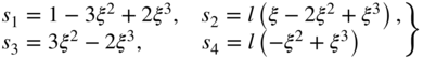
where ![]() . This beam element shape function matrix, which does not allow for shear deformations, was also used by Milner (1981) to study static problems.
. This beam element shape function matrix, which does not allow for shear deformations, was also used by Milner (1981) to study static problems.
Kinematics of the Element
In order to understand the kinematics of the two-dimensional Euler–Bernoulli finite element discussed in this section, some differential geometry results are required. For simplicity, the superscript that indicates the element number is dropped in the following discussion.
The displacement field of the Euler–Bernoulli beam element is function of one spatial coordinate x1 only. For a given, deformed shape of the element, the element centerline defines a space curve. The unit tangent to this space curve is defined by the vector
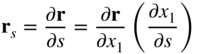
In this equation, s is the arc length. Because rs is a unit vector, that is, ![]() , it follows by differentiating this equation that
, it follows by differentiating this equation that ![]() . This implies that the derivative of the unit tangent with respect to the arc length defines the curvature vector rss, which is perpendicular to rs. The magnitude of the curvature vector κ, called the curvature, measures the rate of change of the tangent vector rs along the arc length. Therefore, the curvature, as previously defined in this chapter, is
. This implies that the derivative of the unit tangent with respect to the arc length defines the curvature vector rss, which is perpendicular to rs. The magnitude of the curvature vector κ, called the curvature, measures the rate of change of the tangent vector rs along the arc length. Therefore, the curvature, as previously defined in this chapter, is
This curvature can be expressed in terms of derivatives with respect to the element spatial coordinate x1(Goetz, 1970; Dmitrochenko and Pogorelov, 2003; Gerstmayr and Shabana, 2006). To this end, recall that ![]() . Because
. Because ![]() has the same direction as the unit tangent rs, one can write
has the same direction as the unit tangent rs, one can write ![]() and
and ![]() . It follows that
. It follows that
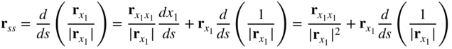
Because rs is a unit vector perpendicular to rss, the curvature can be written upon utilizing the preceding equation as
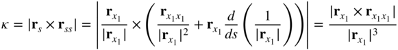
This definition of the curvature does not imply any linearization or simplifications and can be used to define the bending strain in the large-deformation analysis of the Euler–Bernoulli beam element described in this section.
The discussion on the geometry presented in this section shows that if linear interpolation instead of the cubic interpolation is used for this element, the curvature will be zero everywhere inside the element, as previously pointed out. That is, one cannot bend this element. Therefore, a finite element mesh that employs linear interpolation will require a very large number of elements to achieve convergence in beam-bending problems. If quadratic interpolation is used, one obtains, at most, constant curvature. Elements that employ quadratic interpolations lead to zero shear forces as can be demonstrated using simple equilibrium considerations. It is, therefore, recommended to use cubic interpolation to represent beam bending.
Formulation of the Element Elastic Forces
In the case of the Euler–Bernoulli beam element, one can define one gradient vector only because the element assumed displacement field is expressed in terms of one spatial coordinate x1. That is, this element is gradient deficient. Therefore, for this element, the only nonzero strain component is the axial strain, and the shear strain is assumed to be zero. When one or more gradient vectors are missing, the formulation of the elastic forces using the general continuum mechanics approach is not straightforward. Elements that are not gradient deficient have two gradient vectors in the planar analysis and three gradient vectors in the spatial analysis.
Because one spatial coordinate only is used for the Euler–Bernoulli beam element, ![]() cannot be determined using the element assumed displacement field. In this case, the normal to the centerline of the element remains normal, and as a consequence, the shear deformation is assumed to be equal to zero and the cross section of the element is assumed to remain rigid and perpendicular to the element centerline. For this shear nondeformable element, only the strain component ϵ11 can have nonzero value, and it measures only the extensional strain. The bending strain can be defined using the curvature. In the case of two-dimensional elements, which are not gradient deficient, the component ϵ11 is a function of the spatial coordinate x2, and such a component contributes to the bending strain of the finite element, as will be demonstrated in later sections. In this case of shear deformable elements, the use of the curvature definition to define the bending strain energy is not necessary.
cannot be determined using the element assumed displacement field. In this case, the normal to the centerline of the element remains normal, and as a consequence, the shear deformation is assumed to be equal to zero and the cross section of the element is assumed to remain rigid and perpendicular to the element centerline. For this shear nondeformable element, only the strain component ϵ11 can have nonzero value, and it measures only the extensional strain. The bending strain can be defined using the curvature. In the case of two-dimensional elements, which are not gradient deficient, the component ϵ11 is a function of the spatial coordinate x2, and such a component contributes to the bending strain of the finite element, as will be demonstrated in later sections. In this case of shear deformable elements, the use of the curvature definition to define the bending strain energy is not necessary.
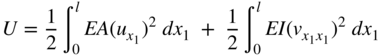
The elastic forces of the two-dimensional Euler–Bernoulli beam element can be obtained by using the virtual work or the strain energy. The virtual work of the elastic forces can be written as
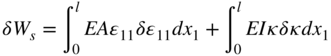
In this equation, l is the length of the element, E is the modulus of elasticity, A is the cross-sectional area, and I is the second moment of area. It is assumed in the preceding equation that the curvature and strain are defined in terms of the reference spatial coordinate x1. Therefore, one can use undeformed geometry data in the integrations of the preceding equation.
The strain energy for the Euler–Bernoulli beam element can be written as
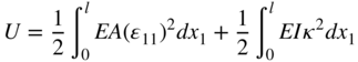
The first integral in the preceding equation represents the strain energy due to the extension, whereas the second integral is the strain energy due to bending. It is important to note that because this element is gradient deficient, one must resort to the curvature definition in order to account for the bending deformation. The curvature definition requires the evaluation of the second derivatives, which is one of the disadvantages of this element. If the element has a complete set of gradients, as it is the case of the shear deformable beam element discussed in the following section, one can use the Green–Lagrange strain tensor to evaluate the elastic forces. This tensor is a function of only first derivatives of the absolute position vector.
The expression of the total strain energy presented in the preceding equation can be used in the large-deformation analysis because no assumptions are made regarding the amount of axial and bending deformations. The strain and curvature can be expressed in terms of the element nodal coordinates. The vector of the elastic forces can be determined using the virtual work as previously described or by using the strain energy as Qs = −(∂U/∂e)T. Different elastic force models can be developed for the Euler–Bernoulli beam element presented in this section, as discussed in the literature (Berzeri and Shabana, 2000).
Special Case
As previously mentioned, the expression of the strain energy presented in this section imposes no restrictions on the amount of the axial and bending deformations of the element. The resulting elastic forces are nonlinear functions of the element nodal coordinates. These nonlinear forces include terms that couple the axial and bending deformations. This coupling has a significant effect on the dynamics of rotating beams. The ANCF element automatically accounts for this coupling when nonlinear strain displacement relationships as the ones employed in this section are used (Berzeri and Shabana, 2002).
In many structural applications, Euler–Bernoulli beam theory has been used for small-deformation analysis. In these structural applications, the rigid-body motion is eliminated. In this special case, an assumption is made that s = x1. Using this assumption, one has ![]() . It follows that the curvature in this special case can be written as
. It follows that the curvature in this special case can be written as
Recall that the curvature vector can be written as
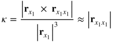
For structural systems in which the rigid-body motion is eliminated, r1 = u is the axial displacement, and r2 = v is the bending displacement. In this case, the strain ϵ11 is approximated as ![]() . Furthermore, the effect of the derivatives of
. Furthermore, the effect of the derivatives of ![]() on the curvature is neglected. The curvature can then be approximated as
on the curvature is neglected. The curvature can then be approximated as ![]() . Using these assumptions, the strain energy that does not account for the coupling between the axial and bending displacements can be written as
. Using these assumptions, the strain energy that does not account for the coupling between the axial and bending displacements can be written as
This expression for the strain energy can only be used in the small-deformation analysis of structural systems, and the use of such an expression in the case of rotating beams can lead to significant errors as the result of the neglect of the effect of the coupling between bending and axial deformations.
5.8 TWO-DIMENSIONAL SHEAR DEFORMABLE BEAM ELEMENT
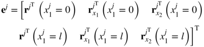
The two-dimensional shear deformable beam element, which was used in several examples in this book, has two nodes. Each node k of element j has six degrees of freedom: two translational coordinates rjk and four gradient coordinates defined by the two vectors ![]() and
and ![]() . The vector of nodal coordinates has 12 elements and is defined at η = 0 as
. The vector of nodal coordinates has 12 elements and is defined at η = 0 as
The shape function matrix for this element is given by
where I is a 2 × 2 identity matrix and the shape functions si, i = 1, 2, …, 6, were obtained in Example 2 as (Omar and Shabana, 2001)
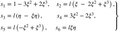
where ![]() and
and ![]() . Note that this fully parameterized element has a complete set of gradient vectors and allows for the deformation of the cross section. Therefore, the element relaxes the assumptions of the Euler–Bernoulli beam theory. Because the cross section does not remain rigid when this element is used, one also obtains a model that is more general than the one based on Timoshenko beam theory.
. Note that this fully parameterized element has a complete set of gradient vectors and allows for the deformation of the cross section. Therefore, the element relaxes the assumptions of the Euler–Bernoulli beam theory. Because the cross section does not remain rigid when this element is used, one also obtains a model that is more general than the one based on Timoshenko beam theory.
Formulation of the Elastic Forces
Because the shear deformable beam element used in this section is not gradient deficient, one can use the general continuum mechanics approach to formulate the element elastic forces. For simplicity, superscript j that indicates the element number will be again dropped in the discussion presented in the remainder of this section. The matrix of position vector gradients of the element can be written in this case as
The Green–Lagrange strain tensor can then be evaluated to define two normal strain components ϵ11 and ϵ22, and one shear strain component ϵ12. The general procedure described previously in this chapter can be employed to define the elastic forces by using the constitutive equations that relate the second Piola–Kirchhoff stress tensor to the Green–Lagrange strain tensor.
The interpolating polynomials used to develop the two-dimensional shear deformable element shape function matrix were introduced in Chapter 1. These polynomials were defined as
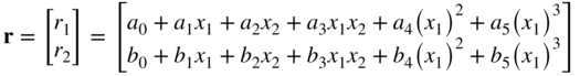
where ai and bi, i = 0, 1, …, 5, are the polynomial coefficients. Note that using this representation, which is cubic in x1 and linear in x2, one can write the vector r as
where r0 = r(x2 = 0) defines the global position of the material points on the centerline of the finite element and ![]() defines the location of the points on the cross section with respect to the centerline. Note that if
defines the location of the points on the cross section with respect to the centerline. Note that if ![]() remains a unit vector perpendicular to the tangent to the centerline, one obtains the Euler–Bernoulli beam model. If, on the other hand,
remains a unit vector perpendicular to the tangent to the centerline, one obtains the Euler–Bernoulli beam model. If, on the other hand, ![]() remains a unit vector that does not remain perpendicular to the tangent to the centerline, one obtains a model similar to the Timoshenko beam model. Using the preceding equation, the strain components can be written as (Sugiyama et al., 2006)
remains a unit vector that does not remain perpendicular to the tangent to the centerline, one obtains a model similar to the Timoshenko beam model. Using the preceding equation, the strain components can be written as (Sugiyama et al., 2006)
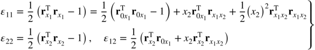
In this equation, ![]() is the tangent to the centerline of the element, and
is the tangent to the centerline of the element, and ![]() describes the rate of change of the gradient vector
describes the rate of change of the gradient vector ![]() with respect to the spatial coordinate x1. Because a linear interpolation with respect to x2 is used, one can show for the finite element described in this section that
with respect to the spatial coordinate x1. Because a linear interpolation with respect to x2 is used, one can show for the finite element described in this section that
where ![]() is the gradient vector
is the gradient vector ![]() defined at node k, k = 1, 2. One can verify that in the case of a rigid-body motion
defined at node k, k = 1, 2. One can verify that in the case of a rigid-body motion ![]() is identically equal to zero. In general, this vector is constant everywhere inside the element, that is, this vector does not depend on the spatial coordinate x1. The fact that the gradient vector
is identically equal to zero. In general, this vector is constant everywhere inside the element, that is, this vector does not depend on the spatial coordinate x1. The fact that the gradient vector ![]() can vary only linearly with respect to x1 regardless of the load applied can introduce excessive stiffness, leading to the locking problem. This problem becomes more serious when thin and stiff structures are modeled. The use of different orders of spatial coordinate interpolations leads to different orders of interpolations for deformations and strain components. When some strain components are restricted to take certain values as the result of a low-order interpolation, the element tends to have unreasonable high stiffness. Different approaches for solving this problem can be used and these approaches, which are well documented in the finite element literature, are briefly discussed in a later section.
can vary only linearly with respect to x1 regardless of the load applied can introduce excessive stiffness, leading to the locking problem. This problem becomes more serious when thin and stiff structures are modeled. The use of different orders of spatial coordinate interpolations leads to different orders of interpolations for deformations and strain components. When some strain components are restricted to take certain values as the result of a low-order interpolation, the element tends to have unreasonable high stiffness. Different approaches for solving this problem can be used and these approaches, which are well documented in the finite element literature, are briefly discussed in a later section.
5.9 THREE-DIMENSIONAL CABLE ELEMENT
The three-dimensional cable element is a simple element that can be efficiently used for cable and belt applications. The element does not have the degree of freedom of the rigid-body rotation about its own axis. Therefore, this element should not be used in applications subject to arbitrary three-dimensional rigid-body rotations. This element, which does not allow for shear deformation, has two nodes. Each node k of element j has six coordinates: three translational coordinates ![]() and three gradient coordinates defined by the vector
and three gradient coordinates defined by the vector ![]() . Therefore, the vector of nodal coordinates has 12 elements and is defined as
. Therefore, the vector of nodal coordinates has 12 elements and is defined as
The interpolation used for the cable element is given by
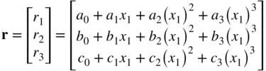
In this interpolation, only one spatial coordinate, x1, is used. The shape function matrix Sj is a 3 × 12 matrix defined as (Gerstmayr and Shabana, 2006)
In this equation, I is a 3 × 3 identity matrix, and
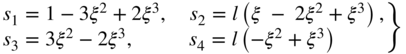
where ![]() and l is the length of the element.
and l is the length of the element.
The cable element is gradient deficient because only one gradient vector is used in the vector of nodal coordinates. In this case, the elastic forces can be formulated using the virtual work or the strain energy. The virtual work of the elastic forces is given as
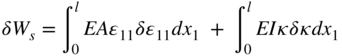
where E is the modulus of elasticity, A is the element cross-sectional area, I is the second moment of area, and κ is the curvature. The effect of the twist of the cable element can also be accounted for by considering the virtual work or the strain energy due to the torsion of the element space curve. Alternatively, the elastic forces of the cable element can be evaluated using the following expression of the strain energy:
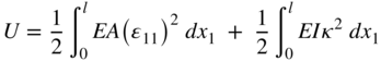
Several investigations have shown that the simple cable element discussed in this section can be very efficient in special applications; particularly, in cable and belt drive applications.
5.10 THREE-DIMENSIONAL BEAM ELEMENT
This is the fully parameterized element, which was used in Example 1. This element that accounts for shear deformation and rotary inertia has two nodes. Each node k of element j has 12 coordinates: 3 translational coordinates ![]() and 9 gradient coordinates defined by the 3 vectors
and 9 gradient coordinates defined by the 3 vectors ![]() ,
, ![]() , and
, and ![]() . Therefore, the element has 24 nodal coordinates, which can be written in a vector form as
. Therefore, the element has 24 nodal coordinates, which can be written in a vector form as
In this equation,
For Node 1, the coordinates are defined at ![]() , and for Node 2, the coordinates are defined at
, and for Node 2, the coordinates are defined at ![]() and
and ![]() . The interpolation polynomials used for this element are given in Example 1. Using these interpolating polynomials, the element shape function matrix is defined as (Yakoub and Shabana, 2001)
. The interpolation polynomials used for this element are given in Example 1. Using these interpolating polynomials, the element shape function matrix is defined as (Yakoub and Shabana, 2001)
where I is the 3 × 3 identity matrix and the shape functions si, i = 1, 2, …, 8, are defined as
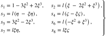
where ![]() .
.
Two methods can be used to formulate the elastic forces of the three-dimensional beam element presented in this section because such an element is not gradient deficient. The first method is based on the general continuum mechanics approach, as previously described in this chapter. In this case, the nonlinear strain displacement relationships are defined in terms of the matrix of the position vector gradients. It is recommended to use the general continuum mechanics approach in the case of very flexible structures because the use of this approach leads to coupled deformation modes that can be significant in the case of large-deformation problems (Hussein et al., 2007). In the case of very thin and very stiff structures, the use of the general continuum mechanics approach is not recommended because the coupled deformation modes can have very high frequencies that lead to deterioration in the element performance. In the case of very thin and stiff structures, one can use an alternate approach, called the elastic line approach (Schwab and Meijaard, 2005). In the elastic line approach, the following gradient vectors are defined at the element centerline:
The following strain and curvature components can also be defined:
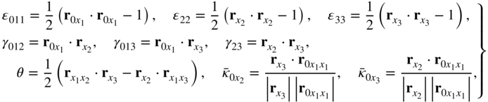
where ϵ011, ϵ22, and ϵ33 are the normal strains; γ012, γ013, and γ23 are the shear strains; θ is the twist; and ![]() and
and ![]() are the expressions of the bending curvature. The strain energy for the element based on the elastic line approach can be written as
are the expressions of the bending curvature. The strain energy for the element based on the elastic line approach can be written as
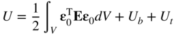
In this equation, E is an appropriate matrix of elastic coefficients, and
The scalars Ub and Ut represent the strain energy due to bending and twist and are defined as

where E and G are, respectively, the modulus of elasticity and modulus of rigidity; ![]() and
and ![]() are the second moments of area about the element x2 and x3 axes, respectively; and Ip is the polar second moment of area. The strain energy U can be used to evaluate the elastic forces, as previously described.
are the second moments of area about the element x2 and x3 axes, respectively; and Ip is the polar second moment of area. The strain energy U can be used to evaluate the elastic forces, as previously described.
Studies have shown that the use of the elastic line approach leads to natural frequencies that are in a good agreement with the analytical solutions that are based on small-deformation assumptions (Schwab and Meijaard, 2005). In the elastic line approach, the coupling between the deformation of the cross section and bending is neglected, thereby leading to a model that is more consistent with the assumptions of the linear theory. When the general continuum mechanics approach is used, the ANCF-coupled deformation modes, as previously mentioned, can introduce high frequencies in the case of thin and stiff structures due to the cross-sectional deformations.
5.11 THIN-PLATE ELEMENT
The three-dimensional thin-plate element is based on Kirchhoff's plate theory. The element, as shown in Figure 7, has four nodal points, and its midsurface is defined by the element spatial coordinates ![]() and
and ![]() . Each node has nine degrees of freedom: three translational coordinates
. Each node has nine degrees of freedom: three translational coordinates ![]() , and six gradient coordinates defined by the two vectors
, and six gradient coordinates defined by the two vectors ![]() and
and ![]() . The element, therefore, has a total of 36 nodal coordinates, which can be written as
. The element, therefore, has a total of 36 nodal coordinates, which can be written as
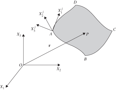
Figure 5.7 Plate element
In this equation,
For Node 1 at point A, the coordinates are defined at ![]() ; for Node 2 at point B, the coordinates are defined at
; for Node 2 at point B, the coordinates are defined at ![]() = a, and
= a, and ![]() ; for Node 3 at point C, the coordinates are defined at
; for Node 3 at point C, the coordinates are defined at ![]() = a,
= a, ![]() , and
, and ![]() ; and for Node 4 at point D, the coordinates are defined at
; and for Node 4 at point D, the coordinates are defined at ![]() ,
, ![]() , and
, and ![]() ; where a and b are the length and width of the element. The element shape function matrix is given by (Dufva and Shabana, 2005)
; where a and b are the length and width of the element. The element shape function matrix is given by (Dufva and Shabana, 2005)
where I is the 3 × 3 identity matrix and the shape functions si, i = 1, 2, …, 12, are as follows:
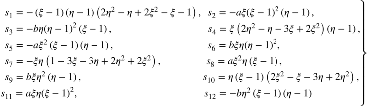
where ![]() .
.
Because for the thin-plate element only the coordinate vector r and the gradient vectors ![]() and
and ![]() are used as nodal coordinates, the element is gradient deficient. The shape function matrix does not depend on the x3 element coordinate, and therefore, the gradient vector
are used as nodal coordinates, the element is gradient deficient. The shape function matrix does not depend on the x3 element coordinate, and therefore, the gradient vector ![]() cannot be used as a coordinate vector. Following Kirchhoff theory, the strain energy of a thin plate can be written as the sum of two terms: one term is due to membrane and shear deformations at the plate midsurface, whereas the other term is due to the plate bending and twist. The strain energy can then be written for a thin plate as follows (Dmitrochenko and Pogorelov, 2003; Dufva and Shabana, 2005):
cannot be used as a coordinate vector. Following Kirchhoff theory, the strain energy of a thin plate can be written as the sum of two terms: one term is due to membrane and shear deformations at the plate midsurface, whereas the other term is due to the plate bending and twist. The strain energy can then be written for a thin plate as follows (Dmitrochenko and Pogorelov, 2003; Dufva and Shabana, 2005):
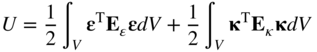
where the curvature vector is ![]() (subscript “0” is omitted here because the shape function matrix does not depend on the element x3 coordinate), and in the case of orthotropic plate, one has
(subscript “0” is omitted here because the shape function matrix does not depend on the element x3 coordinate), and in the case of orthotropic plate, one has
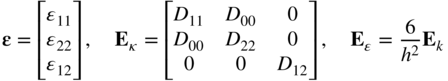
In this equation, h is the plate thickness, Dij = Eijh3/12(1 − v12v21) when i = j, D12 = E12h3/6, D00 = (1/2)(D11v21 + D22v12), Eij are the Young and shear moduli, and vij are the Poisson ratios. The strain components ϵ11, ϵ22, and ϵ12 can be evaluated using the expression for the Green–Lagrange strain tensor, whereas the curvatures can be evaluated using the following expressions.
where the normal n is defined as
Using the strain energy, the elastic forces of the thin-plate element can be calculated using numerical integration methods (Dufva and Shabana, 2005).
5.12 HIGHER-ORDER PLATE ELEMENT
The higher-dimensional plate element employs the full parameterization ![]() ,
, ![]() , and
, and ![]() . The element has four nodes. Each node has 12 coordinates: 3 translational coordinates
. The element has four nodes. Each node has 12 coordinates: 3 translational coordinates ![]() , and 9 gradient coordinates defined by the three vectors
, and 9 gradient coordinates defined by the three vectors ![]() ,
, ![]() , and
, and ![]() . Therefore, the element has 48 nodal coordinates, which can be written in a vector form as
. Therefore, the element has 48 nodal coordinates, which can be written in a vector form as
In this equation,
For Node 1, the coordinates are defined at ![]() ; for Node 2, the coordinates are defined at
; for Node 2, the coordinates are defined at ![]() and
and ![]() ; for Node 3, the coordinates are defined at
; for Node 3, the coordinates are defined at ![]() = a,
= a, ![]() , and
, and ![]() ; and for Node 4, the coordinates are defined at
; and for Node 4, the coordinates are defined at ![]() ,
, ![]() , and
, and ![]() ; where a and b are the length and width of the element. The element shape function matrix is defined as (Mikkola and Shabana, 2003)
; where a and b are the length and width of the element. The element shape function matrix is defined as (Mikkola and Shabana, 2003)
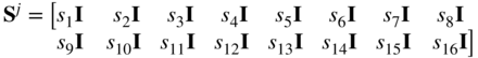
where I is the 3 × 3 identity matrix and the shape functions si, i = 1, 2, …, 16, are as follows:
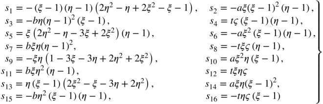
where ![]() ,
, ![]() , and t is the element thickness. The mass matrix of the element is constant, as it is the case in the elements previously discussed in this chapter. The elastic forces can be formulated using the general continuum mechanics approach or the elastic midsurface approach used for the thin-plate element discussed in the preceding section. In the case of thin- and stiff-plate structures, as in the case of other elements, the use of the general continuum mechanics approach introduces high-frequency modes that lead to deterioration of the performance of the element. For such thin and stiff structures, it is recommended to use the elastic midsurface approach, which does not include in the elastic forces coupling between the membrane and bending effects. In the case of very flexible structures, on the other hand, the use of the general continuum mechanics approach for formulating the elastic forces does not lead to deterioration in the element performance, and the use of this approach captures coupled deformation modes that can be significant in the case of large and/or plastic deformations, as previously mentioned in this chapter.
, and t is the element thickness. The mass matrix of the element is constant, as it is the case in the elements previously discussed in this chapter. The elastic forces can be formulated using the general continuum mechanics approach or the elastic midsurface approach used for the thin-plate element discussed in the preceding section. In the case of thin- and stiff-plate structures, as in the case of other elements, the use of the general continuum mechanics approach introduces high-frequency modes that lead to deterioration of the performance of the element. For such thin and stiff structures, it is recommended to use the elastic midsurface approach, which does not include in the elastic forces coupling between the membrane and bending effects. In the case of very flexible structures, on the other hand, the use of the general continuum mechanics approach for formulating the elastic forces does not lead to deterioration in the element performance, and the use of this approach captures coupled deformation modes that can be significant in the case of large and/or plastic deformations, as previously mentioned in this chapter.
5.13 BRICK ELEMENT
A three-dimensional ANCF brick element, with an incomplete polynomial representation, can be developed. This element, shown in Figure 8, has eight nodes. The nodal coordinates ![]() at node k of the finite element
at node k of the finite element ![]() can be defined as
can be defined as ![]() , where
, where ![]() is the absolute position vector at node
is the absolute position vector at node ![]() of the finite element
of the finite element ![]() and
and ![]() ,
, ![]() , and
, and ![]() are the position vector gradients obtained by differentiation with respect to the spatial coordinates
are the position vector gradients obtained by differentiation with respect to the spatial coordinates ![]() , and
, and ![]() , respectively. The displacement field of each coordinate of the brick element can be defined using an incomplete polynomial with 32 coefficients as (Olshevskiy et al., 2013)
, respectively. The displacement field of each coordinate of the brick element can be defined using an incomplete polynomial with 32 coefficients as (Olshevskiy et al., 2013)
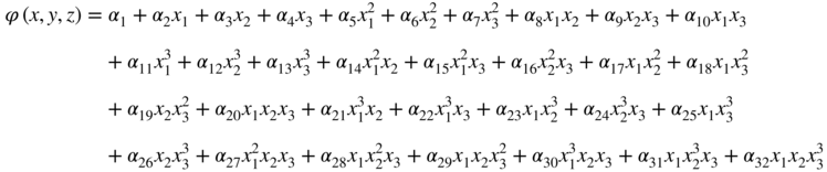
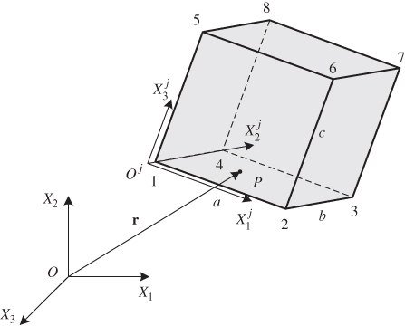
Figure 5.8 ANCF brick element
In this equation, ![]() , are the polynomial coefficients. Using this polynomial description, the shape functions of the ANCF brick element can be derived as follows:
, are the polynomial coefficients. Using this polynomial description, the shape functions of the ANCF brick element can be derived as follows:
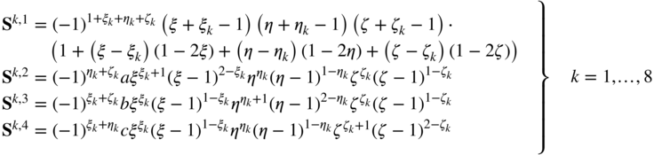
where ![]() , and
, and ![]() are, respectively, the dimensions of the element along the
are, respectively, the dimensions of the element along the ![]() , and
, and ![]() directions,
directions, ![]() ,
, ![]() , and
, and ![]() are the dimensionless nodal locations for node
are the dimensionless nodal locations for node ![]() . The position vector of an arbitrary material point on element
. The position vector of an arbitrary material point on element ![]() can be written as
can be written as
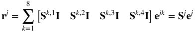
where ![]() is the
is the ![]() identity matrix,
identity matrix, ![]() and
and ![]() are, respectively, the element shape function matrix and the vector of nodal coordinates, which can be written as
are, respectively, the element shape function matrix and the vector of nodal coordinates, which can be written as
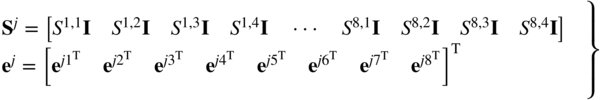
The ANCF brick element described in this section has 96 degrees of freedom and can assume very complex shapes as demonstrated by Wei et al. (2015) in their study of the fluid sloshing problem. Wei et al. (2015) also presented a higher-order ANCF brick element based on a complete polynomial representation.
5.14 ELEMENT PERFORMANCE
All the finite elements presented in this chapter lead to a constant mass matrix and can be used in the large-rotation and large-deformation analysis because nonlinear theory is used with an assumed displacement field that can correctly describe arbitrary large displacements. The use of the two-dimensional Euler–Bernoulli beam and the three-dimensional cable element is restricted to certain applications because they are less general as compared to other elements. Nonetheless, most of the elements described in the preceding sections can be considered as isoparametric elements if the centerlines or the midsurfaces are considered. A finite element is said to be isoparametric if the element shape function can be used to describe both positions (geometry) and displacements of the material points. One can verify that the beam and plate elements presented in this chapter are isoparametric if the positions and displacements of the material points on the centerline or the midsurface are considered. For isoparametric elements, it is straightforward to develop curved elements such as curved beams and shells because one can always use the same displacement field to define stress-free configuration by giving appropriate values for the nodal coordinates. A finite element is said to be subparametric if the order of interpolation used for the positions is lower than the order of interpolation used for the displacement. The element is said to be superparametric if the order of interpolation used for the positions is higher than the order of interpolation used for the displacements. Subparametric and superparametric elements will not be discussed further in this book.
In addition to the elements presented in this chapter, several other elements have been proposed in the literature. Among these elements is the three-dimensional beam element proposed by von Dombrowski (2002) who demonstrated the use of his element in interesting large-deformation applications. In von Dombrowski's element, rotation coordinates are used as nodal coordinates in order to develop an Euler–Bernoulli beam element that accounts for the effect of the rotary inertia. Von Dombrowski's element, which is a more general element as compared to the cable element, is obtained at the expense of not having a constant mass matrix. Because the rotation in this element formulation is assumed to be infinitesimal and only represents rotation about the tangent to the element centerline, the nonlinearity arising from introducing this rotation is not severe and the mass matrix is nearly constant.
Other beam and plate elements were introduced by several authors; some of these elements employ curvature vectors as nodal coordinates. The reader who is interested in this subject can learn about these elements and the formulation of their mass and stiffness matrices from the work of Takahashi and Shimizu (1999), Dmitrochenko and Pogorelov (2003), Garcia-Vallejo et al. (2003), Sopanen and Mikkola (2003), Garcia-Vallejo et al. (2004), and Yoo et al. (2004).
Patch Test
The patch tests are simple tests, which are used to check the convergence of the finite element formulation as well as the computer implementation. These tests can also be used to evaluate the element performance and stability by checking whether or not the element satisfies basic equilibrium requirements. A successful patch test for an element is an indication that if the element is used to model a structure, a refinement of the finite element mesh will produce solutions that converge to the exact solutions. To perform the patch test, one considers a finite element mesh that consists of a small number of elements with at least one node inside the patch. The patch can be subjected to forces or prescribed nodal displacements to develop problems with known exact solutions. For example, boundary nodes can be constrained just enough to eliminate the rigid-body motion of the structure. One can then apply, at the free boundary nodes, loads that correspond to the state of a constant stress. The computed stresses inside the elements are compared with the exact solution to check whether or not the two solutions agree to within the numerical errors. The patch test is repeated to cover all cases of constant stresses relevant to this element. If all the computed stress results agree with the exact solution, the element passes the patch test, and a fine mesh of a structure using this element will produce a solution that converges to the exact one.
One can also examine the strains and displacements to make sure that the computed values are correct. One must also check that in the case of prescribed displacements of the boundary nodes and in the absence of the body forces, the stress and strains must be constant in order for the element to satisfy the partial differential equations of equilibrium. If these conditions are not satisfied, then it is likely that the element assumed displacement field is not correct and/or there is a problem with the computer implementation. It is also recommended to perform an eigenvalue analysis to check that the element has the correct number of rigid-body modes for a given support condition. The eigenvalue analysis should not produce a zero eigenvalue associated with a deformation mode; otherwise, the element will exhibit unstable behavior.
Locking Problem
With regard to the finite element performance, one of the important issues that have been discussed in the literature is the locking problem. Some finite elements exhibit in some applications overly stiff behavior due to two main reasons. First, the order of the polynomial interpolation used for the element is low such that some important modes of deformations cannot be effectively captured. For example, if a linear interpolation is used for a finite element, the curvature which is necessary to describe bending will be zero everywhere inside the element. The use of such low-order finite elements for bending is therefore not recommended because a very large number of elements will be required to solve a simple bending problem. The use of such a fine finite element mesh can be very inefficient in solving beam and plate problems. The second reason for the poor performance of an element is the existence of high-frequency modes that have no significant effect on the solution but lead to a deterioration of the element performance. Such modes can be consistently eliminated using approximation methods based on coordinate reduction as described in the following chapter, or by using analytical methods by introducing kinematic algebraic constraints to prevent the motion in the direction of such stiff modes. The algebraic constraint equations can be used to systematically eliminate these stiff modes from the formulation or can be used to introduce constraint forces that can be expressed in terms of Lagrange multipliers; a subject that has been extensively covered in the MBS dynamics literature (Roberson and Schwertassek, 1988; Shabana, 2013).
As the result of low-order interpolations and the existence of high-frequency modes of deformations, the element performance deteriorates and serious numerical problems can be encountered. There are several types of locking, including volumetric, membrane, and shear locking. For example, most structural materials are nearly incompressible. Changes of the dilatation can be accompanied by large values of stresses that absorb a significant part of the energy and make the element very stiff or lock. Theoretically, an ideal solution to deal with incompressible or nearly incompressible materials is to impose the incompressibility condition as a constraint by assuming that the determinant of the matrix of position vector gradients remains equal to one and does not change. This condition arises from the relationship between the volumes in the current and reference configurations, dv = JdV, where J is the determinant of the matrix of position vector gradients, and dv and dV are, respectively, the volumes in the current and reference configurations. As previously mentioned, imposing the incompressibility condition can be accomplished using two approaches: in the first, a Lagrange multiplier technique is used, whereas in the second, a penalty method is used. The penalty method is easier to use because it is equivalent to adding a force to the equations of motion to guarantee that the incompressibility condition is satisfied. On the other hand, when the Lagrange multiplier technique is used, one must augment the equations of motion with algebraic equations that describe the constraint conditions. This leads to a system of differential and algebraic equations that must be solved simultaneously, making the numerical procedure much more complex as compared to using the penalty method.
The use of the penalty method is equivalent to changing the strain energy of the system by adding another term that enforces the incompressibility condition. Another method used in the finite element literature to solve the locking problems is to use multifield variational principles, which are also called mixed or hybrid principles. In these principles, the stress and strain components that lead to overly stiff behavior are interpolated independently of the displacements. The independent interpolation allows for using higher order for those components that are the source of the locking behavior. Examples of these mixed principles are the Hellinger–Reissner principle and the Hu–Washizu principle: the first is stress based, whereas the second is strain based. The use of these principles allows using different fields for stresses and strains to avoid the locking problem and improve the element behavior in some problems such as beam and plate bending. For this reason, the resulting elements are also called assumed strain or assumed stress elements depending on which variables are interpolated. The drawback of using the mixed principles is that the elements can exhibit instabilities in other fields and, therefore, it is important to check the accuracy of the solution obtained for other field variables.
Shear locking, which is also a source of numerical problems in beam and plate problems, is the result of excessive shear stresses. For thin elements, the cross section is expected to remain perpendicular to the element centerline or midsurface of the element. This is the basic assumption used in Euler–Bernoulli beam theory. Elements that are based on this theory do not allow for shear deformation, and therefore, such elements do not, in general, suffer from the shear locking problem. Examples of these elements are the two-dimensional Euler–Bernoulli beam element and the three-dimensional cable element discussed previously in this chapter. These elements, as demonstrated in the literature, are efficient in thin-beam applications. Shear deformable elements, on the other hand, can suffer from locking problems if they are used in thin structure applications. When these elements are used, the cross section does not remain perpendicular to the element centerline, leading to shear forces. For thin structures, the resulting shear stresses can be very high leading to numerical problems. This problem can be circumvented by using the elastic line or midsurface approaches, the mixed variational principles, or reduced integration methods.
Similarly, some shell-element formulations produce coupling between membrane and bending deformations. In these formulations, a bending of a plate leads to membrane (extension) displacements. This kinematic coupling can lead to the problem of membrane locking, which in turn leads to numerical difficulties when thin shell structures are analyzed. In some applications such as papers and cloths, bending does not produce extension. For these applications, it is recommended to use the thin-plate element formulation, which is based on the elastic midsurface approach. In the formulation of the elastic forces of this element, it is assumed that the bending and extension are not coupled. If, on the other hand, the higher-order fully parameterized plate element is used in thin structural shell applications, it is recommended to use the elastic midsurface approach, the mixed variational principles, and reduced integration methods.
Reduced Integration
One must be careful when speaking of the order of the interpolation and the performance of an element. Although low-order interpolation may necessitate the use of a larger number of elements in order to be able to capture a certain deformation mode, higher-order terms in a polynomial introduce more complex shapes that are associated with high-frequency modes of oscillations. These high-frequency modes can also lead to a deterioration of the element performance. Elimination of these modes can enhance the element performance in some applications. One method, which is recommended in the finite element literature, is to use reduced integration instead of full integration. In the reduced integration, fewer quadrature points are used in the numerical integration of the elastic forces. This is equivalent to using lower-order polynomials to approximate the integrands that appear in the elastic force expressions. Lower-order polynomials have simpler shapes, which are associated with lower modes of oscillations. Elimination of the complex shapes is equivalent to eliminating high frequencies and is equivalent to lowering the element stiffness. This can significantly enhance the element performance. Underintegration, which can be used effectively to eliminate shear locking in some applications, leads to additional computational advantage because it reduces the number of calculations by using fewer quadrature points. Reduced integration, however, should not be used if it leads to mesh instabilities or wrong solutions. It is, therefore, important that the integration rule used is tested in order to make sure that an accurate solution is obtained.
Another form of reduced integration is the selective reduced integration, which can be used to enhance the element performance in some problems. In this integration method, some terms that are the source of locking can be selected and underintegrated, whereas full integration is used for other terms that appear in the expression of the elastic forces. For example, the terms that define the contribution to the elastic forces from the volumetric strains can be underintegrated, whereas terms associated with the deviatoric strains can have a higher order of integration. This method of selective reduced integration can be effective in dealing with volumetric locking in some applications.
Reduced integration if not carefully performed can lead to instabilities. For example, if the deformations at all the selected quadrature points happen to be zero, one obtains zero strain energy for a nonrigid-body mode. In this case, the stiffness matrix is singular and the element exhibits unstable behavior. These types of modes are called in the finite element literature hourglass modes, zero energy modes, or spurious singular modes. These types of modes can be detected using an eigenvalue analysis. In this case, the number of modes of the finite element that have zero eigenvalue is higher than the number of rigid-body modes of the element because the improper selection of the quadrature points leads to a zero eigenvalue associated with a deformation mode.
5.15 OTHER FINITE ELEMENT FORMULATIONS
In this chapter, ANCF finite elements were introduced and discussed. The ANCF approach is suited for the analysis of a general class of problems in which the bodies undergo large rotations including rigid-body rotations. This is a problem that is typical in MBS applications. ANCF finite elements employ absolute position vectors and their gradients as nodal coordinates. There are several reasons, discussed in this section, which motivated introducing this approach and presenting it in this continuum-mechanics-based book. In the finite element literature, there are other types of finite elements that employ different sets of coordinates. In the remainder of this section, we discuss these element formulations in order to further explain the motivation for introducing the formulation presented in this chapter.
Isoparametric Finite Elements
Some elements such as the two-dimensional rectangular and triangular elements and the three-dimensional solid and tetrahedral elements (Zienkiewicz, 1977) employ only position coordinates. These elements can correctly describe rigid-body motion and they are of the isoparametric type because the same shape function can be used to describe the displacement and geometry of the element. Nonetheless, the nodal coordinates do not include rotation variables, which make these elements unsuitable for beam, plate, and shell applications and also unsuitable for many MBS applications where joint constraints between bodies are often formulated in terms of rotation coordinates. Because the continuity of the rotation field at the nodal points is not guaranteed when these isoparametric elements are used, imposing MBS connectivity conditions that allow relative motion is not straightforward. Furthermore, the limitations of these conventional isoparametric elements in the analysis of bending, as the result of the low order of interpolation, are well known and have been discussed in the literature.
Use of Infinitesimal Rotation Coordinates
Another type of finite elements includes elements that employ infinitesimal rotations in addition to translational coordinates as nodal variables. Examples of these conventional finite elements are beam, plate, and shell elements. These elements, which were widely used in many structural applications, cannot correctly describe large rigid-body rotation; they can describe only infinitesimal rigid-body rotation. Because of the use of the infinitesimal rotations as nodal coordinates, one can show that the kinematic equations of these elements employ linearization (Shabana, 1996a). For this reason, these elements have been used in structural dynamics applications in the framework of an incremental solution procedure. It is known, however, that the incremental solutions based on linearized equations eventually diverge from the correct solution of the nonlinear problem. Furthermore, most MBS algorithms that are designed to solve large rigid-body rotation problems are based on nonincremental solution procedure. In order to be able to use these finite elements in MBS algorithms, the finite element FFR formulation was proposed in the early 1980s (Shabana and Wehage, 1981; Shabana, 1982). This approach, which is discussed in detail in the following chapter, leads to correct description of the rigid-body motion of the finite elements that employ infinitesimal rotations as nodal coordinates. The FFR formulation has been primarily used for small-deformation problems because the elements are assumed to undergo small displacements with respect to the floating frame, which may experience an arbitrary rigid-body motion including finite rotations. The FFR formulation remains an effective and efficient tool for modeling the small deformation of flexible bodies because it allows reducing systematically the number of deformation degrees of freedom. This formulation, which will be discussed in more detail in the following chapter, is implemented in most general purpose flexible MBS computer programs.
Perhaps, it is also important to point out that, in MBS applications, one cannot use infinitesimal or finite rotations as nodal coordinates in the interpolation of the rigid-body displacement field. Recall, as shown in Chapter 1, that the rigid-body kinematic equations are defined in terms of trigonometric functions and not in terms of angles. Trigonometric functions can be approximated by angles only when these angles are infinitesimal.
Use of Finite Rotation Coordinates
Another element formulation, which was introduced in the mid-1980s, is based on using two independent fields with finite rotation coordinates as nodal coordinates (Simo and Vu-Quoc, 1986). The resulting elements are capable of correctly describing arbitrary rigid-body displacements. In this formulation, the two independent fields are introduced for the position vector and the finite rotations of the cross section of the finite element. That is, the position and rotations are obtained from independent interpolations. As demonstrated in this book, using the polar decomposition theorem, the rotation field can be defined using the matrix of position vector gradients. That is, the position vector field is sufficient to determine the rotations of infinitesimal volumes. The use of independent displacement and rotation fields, therefore, can lead to a problem of coordinate redundancy and inconsistency in the definition of the rotation variables (Ding et al., 2014). Formulations that suffer from this problem of coordinate redundancy can lead to numerical problems in the analysis of large rotations, particularly large rigid-body rotations. For instance, some of these formulations do not automatically satisfy the principle of work and energy, and special measures must be taken in the numerical integration routines in order to satisfy this principle. On the other hand, because the ANCF position vector field is used to determine the gradients that define the rotation field, such a problem is not encountered, and ANCF finite elements automatically satisfy the principle of work and energy without the need for special measures as demonstrated in the literature (Campanelli et al., 2000).
5.16 UPDATED LAGRANGIAN AND EULERIAN FORMULATIONS
In this chapter, a total Lagrangian large-deformation finite element formulation was considered. Integrations and differentiations are defined with respect to the Lagrangian coordinates, and stress and strain measures are defined with respect to the reference configuration. The ANCF finite elements presented in this chapter can also be used with an updated Lagrangian formulation. In this case, one uses stress and strain measures defined in the current configuration. Furthermore, the differentiations are defined with respect to the coordinates r, whereas the integrations are defined using the current volumes and areas. In principle, as discussed in Chapter 3, the total and updated Lagrangian formulations are equivalent, and one formulation can be obtained from the other using a coordinate transformation. Therefore, the choice of a formulation is a matter of convenience or preference, and in some cases, some variables defined in the current configuration are used with the total Lagrangian formulation and vice versa. For this reason, the updated Lagrangian formulation will not be discussed further in this book. The reader interested in the updated Lagrangian formulation can consult the literature on the nonlinear finite element method.
Whereas in the Lagrangian formulations, the finite element nodal points move as the result of the applied forces, in the Eulerian formulations with fixed mesh, the nodes are fixed since the focus is on a region of the continuum that is defined by the vector r. One then does not follow the motion of a material point that has coordinates x in the reference configuration; instead, the focus is on a point through which the material flows, and the interest is to determine the behavior of the continuum when the material passes by this point, which is fixed in space. The Eulerian description is more convenient to use in the case of fluid dynamics, whereas the Lagrangian description is used more often in solid mechanics. In the Eulerian formulations, three sets of variables are often used; the density ρ, the stresses σ, and the velocities v. In order to solve for these three sets of variables, three sets of equations are used. These equations are the continuity or conservation of mass equation, the constitutive equations, and the equations of motion. The constitutive equations are often expressed in the rate form. These three sets of equations can be written in the following form:
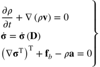
In this equation, ρ is the density defined in the current configuration, v is the velocity vector, σ is the stress tensor, D is the rate of deformation tensor, fb is the vector of body forces, and a is the acceleration vector. The continuity equation can also be written in the following alternate form:
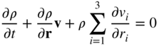
In the Eulerian formulations, independent interpolations are used for the density, stresses, and velocities. One can then write for element j the following finite element description:
In this equation, Sj is the element shape function used for the displacement, ej is the vector of element position nodal coordinates, ![]() is the shape function used for the stresses,
is the shape function used for the stresses, ![]() is the set of stress nodal variables,
is the set of stress nodal variables, ![]() is the density shape function, and
is the density shape function, and ![]() is the set of density nodal variables. Because
is the set of density nodal variables. Because ![]() , Equation 140 can be used to define the following virtual changes:
, Equation 140 can be used to define the following virtual changes:
As previously mentioned, in the Eulerian formulation with fixed mesh, the nodal points are assumed to be fixed. On fixed boundaries in fluid applications, the velocities at the boundary nodal points are assumed to be zero.
In order to obtain the discrete equations, one can multiply the first equation in Equation 138 by δρj, the second equation by δσj, and the third equation by δvj; integrating over the domain of the element and using Equation 141, one can show that the finite element discrete equations in the Eulerian formulation can be written as
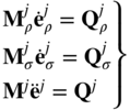
where ![]() , and Mj are coefficient matrices; and
, and Mj are coefficient matrices; and ![]() , and Qj are vectors that can depend on the unknown variables. In obtaining Equation 142, the integration is carried out over a fixed element domain in the case of a fixed mesh. Note that in the ANCF Eulerian formulation discussed in this chapter, the mass matrix Mj depends on the density, which is a function of time in the case of compressible materials or fluid. Consequently, this mass matrix is not constant as in the case of the Lagrangian formulations. If the material is incompressible, the density is not a function of time, and the continuity equation is simplified. In this case, ANCF finite elements lead to a constant mass matrix. In general, the three sets of equations given by Equation 142 are solved simultaneously to determine the values of the coupled variables of the continuum at the nodes. In the case of fluid dynamics, there are several simulation scenarios that depend on the fluid conditions. In some of these scenarios, the governing equations given in Equation 139 can be simplified.
, and Qj are vectors that can depend on the unknown variables. In obtaining Equation 142, the integration is carried out over a fixed element domain in the case of a fixed mesh. Note that in the ANCF Eulerian formulation discussed in this chapter, the mass matrix Mj depends on the density, which is a function of time in the case of compressible materials or fluid. Consequently, this mass matrix is not constant as in the case of the Lagrangian formulations. If the material is incompressible, the density is not a function of time, and the continuity equation is simplified. In this case, ANCF finite elements lead to a constant mass matrix. In general, the three sets of equations given by Equation 142 are solved simultaneously to determine the values of the coupled variables of the continuum at the nodes. In the case of fluid dynamics, there are several simulation scenarios that depend on the fluid conditions. In some of these scenarios, the governing equations given in Equation 139 can be simplified.
It is important, however, to point out that a total Lagrangian formulation that employs ANCF finite element can still be used in some fluid applications such as in the case of sloshing problems (Wei et al., 2015). In such applications, the effect of the fluid motion on vehicle dynamics is the primary concern. When ANCF finite elements are used, the expression for the inertia forces remains as previously discussed in this chapter. Regardless of the magnitude of the fluid displacement, the mass matrix remains constant, and the centrifugal and Coriolis forces are identically zero. The stress forces can be determined using the fluid constitutive equations as discussed in Chapter 4. Figure 9 shows the fluid simulation results obtained by Wei et al. (2015). These results are obtained using the ANCF solid element, which ensures the continuity of the displacement gradients at the nodal points (Olshevskiy et al., 2013). The total Lagrangian nonincremental liquid sloshing solution procedure proposed by Wei et al. (2015) can be used to avoid the difficulties of integrating most of fluid dynamics formulations, which are based on the Eulerian approach, with MBS dynamics formulations, which are based on a total Lagrangian approach. The proposed total Lagrangian FE fluid dynamics formulation, which can be systematically integrated with computational MBS algorithms, differs significantly from the conventional FE or finite volume methods, which are based on an Eulerian representation that employs the velocity field of a fixed control volume in the region of interest. The ANCF fluid equations are expressed in terms of displacement and gradient coordinates of material points, allowing for straightforward implementation of kinematic constraint equations and for the systematic modeling of the interaction of the fluid with the external environment or with rigid and flexible bodies. The fluid incompressibility conditions and surface traction forces are considered and derived directly from the Navier Stokes equations. Wei et al. (2015) formulated the fluid problem using two ANCF brick elements, one is obtained using an incomplete polynomial representation and the other is obtained from a B-spline volume representation. The new approach, in addition to ensuring the continuity of the displacement gradients at the nodal points, allows for imposing higher degree of continuity across the element interface by applying algebraic constraint equations that can be used to eliminate dependent variables and reduce the model dimensionality.
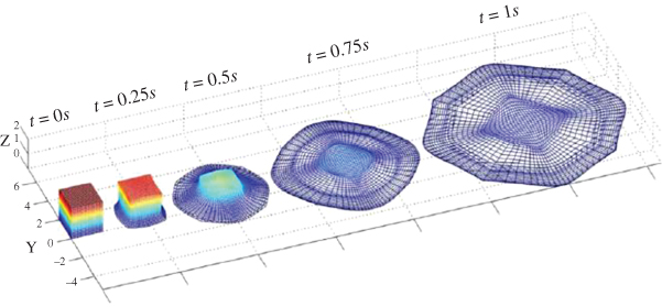
Figure 5.9 ANCF total Lagrangian fluid simulation (Wei et al., 2015)
5.17 CONCLUDING REMARKS
In this chapter, an approach for the large displacement analysis of continuous systems is described. In order to be able to use this approach to develop accurate models for engineering and physics systems, it is necessary to understand some basic geometry and analysis concepts.
ANCF Finite Elements
The following characteristics define the ANCF solution framework:
- 1. The problem must be a dynamics problem that requires addressing the formulation of the inertia forces, which are expressed in terms of a constant inertia matrix and, therefore, the Coriolis and centrifugal forces are identically zero.
- 2. The elements must be of higher order in order to provide the option for imposing continuity on gradient vectors. The vector of nodal coordinates of ANCF finite elements can consist of position and gradient coordinates and the gradients must be interpreted correctly during the entire solution procedure. Conventional
 finite elements do not ensure continuity of the gradient or rotation fields. As it is known continuity of the gradients ensures continuity of the rotations. The converse, however, is not, in general, true.
 - 3. The finite elements must correctly describe an arbitrary rigid body motion including arbitrary finite rotations using the assumed displacement field
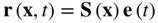 , where
  is the global position vector of an arbitrary point on the element,
  is the element shape function matrix,
  is the vector of nodal coordinates,
  is the vector of the element spatial coordinates, and
  is time.
When using ANCF finite elements, the equations of motion can be solved nonincrementally and, therefore, there is no need for the use of the corotational approach, which was introduced to remedy the problems associated with finite elements that employ infinitesimal rotations. In the FE literature, there has been frequent reference to gradients and slopes. Nonetheless, all the above conditions are not often met as the result of improper treatment of the gradients, the use of incremental procedures, and/or the focus on static procedures without addressing the formulation of the element inertia when the element experiences arbitrary finite rotations (Betsch and Stein, 1995; Milner, 1981).
Constrained Motion
As discussed in this chapter, ANCF finite elements can be used as the basis for a nonincremental solution procedure that allows for developing new computer models with significant details. One example of these models is the tracked vehicle shown in Figure 10. The links of the track chains of this vehicle are modeled as flexible bodies connected by pin (revolute) joints that allow relative rotation as well as relative deformations between the chain links. This detailed vehicle model was successfully developed using ANCF finite elements and computational MBS algorithms (Hamed et al, 2015; Wallin et al., 2013). Using ANCF finite elements, linear connectivity conditions, that define the pin (revolute) joints, were developed, allowing eliminating the dependent variables at a preprocessing stage (Garcia-Vallejo et al, 2003; Hamed et al., 2015). The two tracks of the vehicle can be treated as one ANCF finite element mesh since ANCF finite elements allow for arbitrarily large displacements. The track chains mass matrix remains constant and the centrifugal and Coriolis forces remain equal to zero. The development of such a heavily constrained model, in which the algebraic connectivity conditions are eliminated at a preprocessing stage, using ANCF finite elements is straightforward.
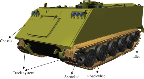
Figure 5.10 Tracked vehicles
ANCF Reference Node
Another important concept that has been used effectively in modeling complex system is the ANCF reference node (Shabana, 2015a,b). The ANCF reference node is a node that is not associated with a particular ANCF finite element. This node can be used for assembling rigid and structural components. Such a node can also be used to describe a rigid body by imposing six rigidity constraints that eliminate the deformation modes of the reference node. The reference node can be used to develop new tire assembly models and can be used also to develop an MBS submodel at a preprocessing stage as shown in Figure 11 (Shabana, 2015a,b).
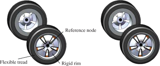
Figure 5.11 Tire assembly
Deformation Modes
As discussed in the literature, and also in this book, fully parameterized ANCF finite elements may exhibit locking behavior, particularly in the case of thin and stiff structures. Nonetheless, the use of such fully parameterized ANCF finite elements is necessary in order to be able to capture correct physics in many applications. For example, excessive axial and bending forces lead to change in the cross-sectional dimensions of beam-like structure. Formulations that assume rigid cross section, from the outset, cannot be used to capture this physics behavior. In the finite element literature, many solutions were proposed to solve the locking problem. Some of the locking-solution techniques can be applied in the case of fully parameterized ANCF finite elements, allowing for developing new models that correctly capture the physics of the problem under consideration.
PROBLEMS
-
1 Verify the expressions of the shape functions presented in Example 1.
-
2 Show that the displacement field used in Example 1 can describe an arbitrary rigid-body motion.
-
3 Verify the expressions of the shape functions presented in Example 2, and show that the displacement field used in Example 2 can describe an arbitrary rigid-body motion.
-
4 Show that, by using the Cholesky factorization of the symmetric mass matrix, one can define a new set of coordinates that lead to an identity mass matrix.
-
5 Show that the virtual changes in the Green–Lagrange strains can be written in terms of the virtual changes of the position vector gradients. Show also that the virtual changes in the position vector gradients can be written in terms of the virtual changes of the finite element nodal coordinates.
-
6 A force vector F(t) = [F1(t) F2(t)]T applied at a point defined by ξ = 0.5 of the two-dimensional Euler–Bernoulli beam element defined in Section 7. Define the vector of nodal forces due to the application of this force vector. Define also the vector of nodal forces if this force vector is applied at a point defined by ξ = 1. Discuss the nodal forces associated with the gradient coordinates of this element. Repeat this problem using the two-dimensional shear deformable element.
-
7 In the two-dimensional case, define the relationship between the virtual change in the rotation and the virtual change of the gradient coordinates at the node for both Euler–Bernoulli and shear deformable beam elements. Use this relationship to define the relationship between the Cartesian moment and the forces associated with the gradient coordinates of these two elements.
-
8 Develop the mass matrix of the two-dimensional Euler–Bernoulli beam element discussed in Section 7.
-
9 A force vector F(t) = [F1(t) F2(t) F3(t)]T is applied at a point defined by ξ = 0.5 of the cable element presented in Section 9. Define the vector of nodal forces due to the application of this force vector. Define also the vector of nodal forces if this force vector is applied at a point defined by ξ = 1. Discuss the nodal forces associated with the gradient coordinates of this element. Repeat this problem using the three-dimensional shear deformable element.
-
10 Obtain the expression for the nodal forces due to gravity in the case of the following finite elements: (1) two-dimensional Euler–Bernoulli beam element, (2) two-dimensional shear deformable beam element, (3) cable element, (4) three-dimensional shear deformable element, and (5) thin-plate element.
-
11 Obtain the mass matrix of the three-dimensional cable element.