CHAPTER 4
CONSTITUTIVE EQUATIONS
The kinematic and force equations developed in the preceding two chapters are general and applicable to all types of materials. The mechanics of solids and fluids is governed by the same equations, which do not distinguish between different materials. The definitions of the strain and stress tensors, however, are not sufficient for describing the behavior of continuous bodies. The force–displacement relationship or equivalently the stress–strain relationship is required in order to be able to distinguish between different materials and solve the equilibrium equations. The continuum displacements depend on the applied forces, and the force–displacement relationship depends on the material of the continuum. To complete the specification of the mechanical properties of a material, one needs an additional set of equations called the constitutive equations, which serve to distinguish one material from another. The form of the constitutive equations of a material should not be altered in the case of a pure rigid-body motion. These equations, therefore, must be objective, and should not lead to change in the work and energy of the stresses under an arbitrary rigid-body motion. Using the constitutive equations, the partial differential equations of equilibrium obtained in the preceding chapter can be expressed in terms of the strains. Using the strain–displacement relationships, these equilibrium equations can be expressed in terms of displacements or position coordinates and their time and spatial derivatives. If the continuum density is considered as an unknown variable, as it is the case in some fluid applications, the continuity equations can be added to the resulting system of partial differential equations in order to have a number of equations equal to the number of unknowns.
If the constitutive equations of a material depend only on the current state of deformation, the behavior is said to be elastic. If the stresses can be derived from a stored energy function, the material is termed hyperelastic or called Green elastic material. A more general class of materials, for which the stresses cannot be derived from a stored energy function, is called Cauchy elastic material. For hyperelastic materials, the work done by the stresses during a deformation process is path independent. That is, the work done depends only on the initial and final states. For such systems, the continuum returns to its original configuration after the load is released. For viscoelastic materials, on the other hand, the work done during a deformation process is path dependent due to the dissipation of energy during the deformation process. The constitutive equations of viscoelastic materials are formulated in terms of rate of deformation measures in order to account for the energy dissipation.
In this chapter, the general constitutive equations of the materials are presented and systematically simplified in order to obtain the important special case of isotropic materials. It is shown that for isotropic materials that satisfy certain homogeneity and symmetry properties, the constitutive equations depend only on two constants called Lame's constants. Materials described by this model are called Hookean materials. The Hookean material model can be used in the case of small deformations. Other models, which are more appropriate for large deformations, such as the Neo–Hookean and the incompressible Mooney–Rivlin material models, are discussed. These nonlinear material models can be more accurate and lead to more efficient solutions in some applications, particularly when the assumption of linearity can no longer be used. The constitutive equations for viscoelastic materials and fluids are also discussed in this chapter. The behavior of elastic–plastic materials is discussed in a later chapter of this book.
4.1 GENERALIZED HOOKE'S LAW
The analysis presented in the preceding chapter shows that the second Piola–Kirchhoff stress tensor is the only tensor considered so far in this book that is directly associated in the virtual work and energy equations to a strain measure that can be expressed in a nondifferential form. Therefore, in this chapter, for the most part, the constitutive equations are assumed to relate the second Piola–Kirchhoff stress tensor and the Green–Lagrange strain tensor. In many inelastic formulations, however, constitutive equations in rate form are often expressed in terms of other stress and strain measures.
In this section, the general linear relationship between the stress and strain components is developed. As discussed in the preceding chapter, it is important to use consistent stress and deformation measures in the definition of the elastic forces. In this section, the Green–Lagrange strain tensor is used with the second Piola–Kirchhoff stress tensor to define a linear constitutive model. Nonetheless, one can always develop constitutive relationship between different stress and strain measures because these measures are related as previously mentioned. In this section, unless stated otherwise, σ is used for simplicity to denote the stress measure, which is assumed to be the second Piola–Kirchhoff stress measure, whereas ϵ is used to denote the Green–Lagrange strain measure. The goal is to develop the relationship σ = σ (ϵ). In developing this relationship, it is important to distinguish between homogeneous and isotropic materials. A material is said to be homogeneous if it has the same properties at every point. That is, the elastic properties are not function of the location of the material points. In the case of isotropic materials, on the other hand, the elastic properties are assumed to be the same in all directions. That is, a coordinate transformation does not affect the definition of the elastic constants.
It has been found experimentally that for most materials, the measured strains are functions of the applied forces. For most solids, the strains are proportional to the applied forces, provided that the load does not exceed a given value known as the elastic limit. This experimental observation can be stated as follows: the stress components at any point in the body are linear functions of the strain components. This statement is a generalization of Hooke's law and does not apply to viscoelastic, plastic, or viscoplastic materials. The generalization of Hooke's law may thus be written, using vector and matrix notation instead of tensor notation, as
where Em is the matrix of elastic coefficients, and σv and ϵv are, respectively, the stress and strain components written in a vector form and defined as
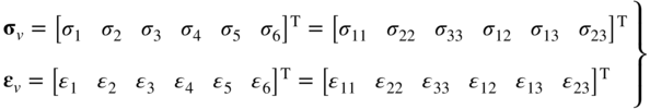
One may also write Equation 1 using tensor notation as
In this equation, σ and ϵ are, respectively, the second-order stress and strain tensors and E is the fourth-order tensor of the elastic coefficients. When tensor notations are used, the stresses are defined according to the rule of the double contraction as ![]() , where in this equation
, where in this equation ![]() are the elements of the fourth-order tensor
are the elements of the fourth-order tensor ![]() , that is,
, that is, ![]() . In this chapter, the vector and matrix form of Equations 1 and 2 are sometimes used in order to simplify the derivations and take advantage of the symmetry of the stress and strain tensors. It is important, however, to recognize that Equations 1 and 3 are equivalent.
. In this chapter, the vector and matrix form of Equations 1 and 2 are sometimes used in order to simplify the derivations and take advantage of the symmetry of the stress and strain tensors. It is important, however, to recognize that Equations 1 and 3 are equivalent.
It was shown in the preceding two chapters that the Green–Lagrange strain tensor and the second Piola–Kirchhoff stress tensor do not change under an arbitrary rigid-body motion and the product σP2: ϵ satisfies the objectivity requirement. It is important, therefore, that the constitutive law used satisfies the objectivity requirement, which is automatically satisfied for linear isotropic elastic materials since the tensor of elastic coefficients E is constant, as demonstrated in this chapter.
In the case of a general material, the matrix of elastic coefficients Em has 36 coefficients. This matrix can be written in its general form as follows:

The coefficients eij, i, j = 1, 2,…, 6, define the material elastic properties when the behavior is assumed to be linear. The number of independent coefficients can be reduced if the material exhibits special characteristics as discussed in the following sections.
4.2 ANISOTROPIC LINEARLY ELASTIC MATERIALS
Let U be the strain energy, per unit volume, that represents the work done by the internal stresses. Using the definition of the work presented in the preceding chapter, one then has
which implies that
This equation can be written more explicitly in terms of the stress and strain components as

The preceding two equations when combined with the constitutive equations (Equation 3) imply
Note that this relationship is valid only for linearly elastic materials in which the elastic coefficients are assumed to be independent of the strains. This equation shows that

Here, for simplicity, a single subscript is used for the strain components according to the definitions of Equation 2. Equation 9 implies that
This equation shows that for linearly elastic materials, the matrix of elastic coefficients is symmetric and there are only 21 distinct elastic coefficients for a general anisotropic linearly elastic material. This result is obtained based on energy considerations using the basic definition of the work of the elastic forces obtained in the preceding chapter and as defined by Equation 5.
4.3 MATERIAL SYMMETRY
In some structural materials, special kinds of symmetry may exist. The elastic coefficients, for example, may remain invariant under coordinate transformations. In this section, a reflection transformation and a proper orthogonal transformation due to rotations are considered. The obtained transformation results are used to reduce the number of unknown elastic coefficients.
Reflection
Consider the reflection with respect to the X1X2 plane given by the following transformation:

The transformed stress and strain tensors ![]() and
and ![]() are given, respectively, by
are given, respectively, by

Using this transformation for the stresses and strains, one obtains

and

If the elastic coefficients are assumed to be invariant under the reflection transformation, that is, the elastic properties at two material points on the opposite sides of the X1X2 plane are the same, one can write, for example, ![]() as
as
Using the result of the reflection transformation, one can write
Comparing the preceding two equations, one obtains ![]()
In a similar manner by considering other stress components, one can show that
Therefore, the number of independent elastic coefficients for a material that possesses a plane of elastic symmetry reduces to 13. If this plane of symmetry is the X1X2 plane, that is, the elastic properties are invariant under a reflection with respect to the X1X2 plane, the matrix Em of elastic coefficients can be written as

If the material has two mutually orthogonal planes of symmetry, one can show that e41 = e42 = e43 = e65 = 0 and the matrix of elastic coefficients reduces to

That is, the number of elastic coefficients is reduced to nine.
Rotations
In some materials, the elastic coefficients eij remain invariant under a rotation through an angle α about one of the axes, that is, the values of these coefficients are independent of the set of the rectangular axes chosen. For example, the transformation matrix A in the case of a rotation about the X3 axis is given by

One may write expressions for the transformed stress and strain tensors for different values of α and proceed as in the case of reflection to show that in the case of an isotropic solid there are only two independent constants, denoted by λ and μ. One can show that in this case

The two elastic constants λ and μ are known as Lame's constants. These two constants do not have to take the same values at every point on the continuum unless the material is assumed to be homogeneous. The case of homogeneous isotropic materials is discussed in the following section.
4.4 HOMOGENEOUS ISOTROPIC MATERIAL
If the material is homogeneous, λ and μ are constants at all points. The matrix Em of elastic coefficients can be written in the case of an isotropic homogeneous material in terms of Lame's constants as

In this case, the relationship between the stresses and strains can be written explicitly as

where
is called the dilatation. The strains can be written in terms of the stresses (inverse relationship) as follows:

where
and

The constants μ, E, and γ are, respectively, called the modulus of rigidity or shear modulus, Young's modulus or modulus of elasticity, and Poisson's ratio. In terms of these elastic coefficients, Equation 24 can be written as

Poisson Effect and Locking
Lame's constants can also be written in terms of the modulus of elasticity and Poisson ratio as

Equations 26 and 29 show that the effect of the Poisson ratio is to produce stresses that couple the stretch deformations in different directions. That is, if the Poisson ratio is equal to zero, the normal stresses are related to the normal strains by the equation σii = Eϵii, i = 1, 2, 3, which shows that the normal stress in one direction is independent of the normal strains in the other two directions. Furthermore, the value of the Poisson ratio cannot exceed 0.5. If the Poisson ratio becomes close to 0.5, the elastic coefficient associated with the dilatation ϵt becomes very large, producing high stiffness that tends to resist any volume change. When the continuum equations are solved numerically, this high stiffness can be a source of problems and introduces what is referred to as locking. In fact, there are several types of locking including volumetric, shear, and membrane locking associated with different materials and structural elements. For instance, the volumetric locking can be explained by using the first equation in Equation 24. Using this equation, one can show that σ11 + σ22 + σ33 = (3λ + 2 μ)ϵt. This equation shows that the hydrostatic pressure p, in the case of small deformation, can be written as p = {(3λ + 2 μ)ϵt }/3, which upon the use of Equation 30 can be written as p = Kϵt, where K is the Bulk modulus defined as K = E/{3(1 − 2γ)}. The equation p = Kϵt, defines the relationship between the hydrostatic pressure and the dilatation. If the Poisson ratio approaches 0.5, the bulk modulus becomes very large leading to a very large stiffness coefficient associated with the volumetric change.
The locking problem will be revisited in Chapter 5 when large-deformation finite element formulations are discussed. It is important, however, to point out that many of the existing finite element formulations for structural elements such as beams do not take into consideration Poisson effects. This is mainly due to the fact that the element cross sections in these formulations are assumed rigid and are not allowed to deform. The large-deformation finite element formulation discussed in Chapter 5 allows taking into consideration the Poisson effect because the element cross section is allowed to deform. Such a formulation allows for the use of general constitutive models as the ones discussed in this chapter, and therefore, coupling between different displacement modes such as the bending deformation and the stretch of the cross section can be taken into account in the case of beam, plate, and shell problems.
Stress and Strain Invariants
Using Equation 24 and the definitions of the symmetric strain and stress tensor invariants presented in the preceding two chapters, one can show that the stress invariants J1, J2, and J3 are related to the strain invariants I1, I2, and I3 by the following equations (Boresi and Chong, 2000):

Some material constitutive models are formulated in terms of the invariants of deformation measures as discussed later in this chapter.
Using Equation 24, the strain energy density function can be written in terms of Lame's constants and the strain components as
Recall that the invariants of the symmetric strain tensor are defined in terms of the strain components as

This equation shows that I1 is a function of the normal strains, whereas I2 depends on the normal and shear strain components. Using the preceding two equations, one can show that the strain energy density function for linearly elastic and isotropic materials can be written in terms of the invariants of the strain tensor as
The coefficient of the square of the dilatation in this strain energy density expression can be written as

This equation demonstrates once again the numerical problems that can be encountered when dealing with incompressible and nearly incompressible materials.
Invariants of the deformation measures can have a clear physical meaning that explains the stiffness coefficients that enter into the formulation of the material constitutive equations. For example, I3 is a measure of the change of volume, whereas the dilatation I1 can be a measure of the stretch. For isotropic materials, it is sometimes more convenient to use directly the invariants of the deformation measure to develop the constitutive equations. For this reason, some identities related to these invariants are discussed in detail in the following section, whereas the use of these identities in developing constitutive models for other material types is discussed in Section 5.
Plane-Stress and Plane-Strain Problems
If σ13, σ23, and σ33 are equal to zero, that is, σ13 = σ23 = σ33 = 0, one has the case of plane stress. In this case, Equation 26 yields

Using these equations, one can show that the constitutive equations for linearly elastic isotropic materials can be written as

The assumptions of plane stress are made in several applications such as in the analysis of thin plates. If the interest is focused on the deformation of the plate midsurface in response to applied forces, the normal and shear stresses in the direction of the plate thickness can be neglected.
In the case of plane strain, one has ϵ13 = ϵ23 = ϵ33 = 0. Using Equation 24, one has

The constitutive equations can be written in this case as

Recall that the stress–strain relationships presented in this section are based on the assumption of linear behavior of the materials. These relationships, therefore, cannot be used directly in the case of materials that do not exhibit linear behavior based on the assumptions described in this chapter. Other constitutive relationships must be used for nonlinear materials, materials that have directional properties, or plastic and viscoelastic materials.
Finite Dimensional Model
As in the case of the inertia and body forces, one can systematically develop, using approximation methods, an expression of the stress forces of the infinite-dimension continuum in terms of a finite set of coordinates. To this end, the strain energy expression or the virtual work of the elastic forces can be used. The strains can be expressed in terms of the position vector gradients. The position vector gradients can be written in terms of the time-dependent coordinates. Using the constitutive equations, the virtual work or the strain energy can be expressed in terms of the coordinates used in the assumed displacement field. This systematic procedure is described by the following example.
Generalized Elastic Forces
As explained in the preceding chapter, the last equation in the preceding example can be used to write the virtual work of the elastic forces in terms of the virtual changes in the position vector gradients as ![]() , where
, where ![]() is the matrix of position vector gradients,
is the matrix of position vector gradients, ![]() is the vector of spatial coordinates, and
is the vector of spatial coordinates, and ![]() ,
, ![]() , and
, and ![]() are the columns of the stress tensor. When using the finite dimensional model based on the kinematic description
are the columns of the stress tensor. When using the finite dimensional model based on the kinematic description ![]() used in the preceding example, one has
used in the preceding example, one has ![]() . It follows that the virtual work of the elastic forces can be written as
. It follows that the virtual work of the elastic forces can be written as ![]() , which can be written as
, which can be written as ![]() , where
, where ![]() is the vector of elastic generalized forces. As mentioned in the preceding chapter, this vector is, in general, a highly nonlinear function of the coordinates, and therefore, numerical integration is often required to calculate this force vector.
is the vector of elastic generalized forces. As mentioned in the preceding chapter, this vector is, in general, a highly nonlinear function of the coordinates, and therefore, numerical integration is often required to calculate this force vector.
Homogeneous Displacement
Some of the finite elements used in the literature yield constant strains. That is, the strain components are the same at every material point. These elements, which are defined using linear displacement field, are called constant-strain elements. As discussed in the preceding chapter, in the case of homogeneous displacements, the matrix of position vector gradients J is the same everywhere throughout the continuum. A special example of this motion is the rigid-body motion, in which J represents an orthogonal matrix. Because in the case of homogeneous displacements, the strain components are the same at all material points, the stress tensor is independent of the location at which this tensor is evaluated if the matrix of the elastic coefficients is independent of the location, as in the case of isotropic materials. One, therefore, has ![]() .
.
4.5 PRINCIPAL STRAIN INVARIANTS
In the case of isotropic materials, the constitutive behavior must be the same in any material direction. This means that the relationship between the potential function U and the Green–Lagrange strain tensor ϵ, or equivalently the right Cauchy–Green deformation tensor Cr, is independent of the chosen material axes. As a consequence, the potential function U must depend only on the invariants of ϵ, as demonstrated in the preceding section or equivalently on the invariants of the right Cauchy–Green deformation tensor Cr. In this case, one can write the potential function as
where I1, I2, and I3 are considered here to be the invariants of Cr defined as
These invariants can be written in terms of the eigenvalues λ1, λ2, and λ3 of Cr as

In the analysis of the large deformation, the second Piola–Kirchhoff stress tensor can be obtained from the potential function U. Recall that the right Cauchy–Green deformation tensor can be written in terms of the Green–Lagrange strain tensor as Cr = 2ϵ + I. Because ϵ and σP2 are symmetric, the second Piola–Kirchhoff stress tensor can then be written as

The derivatives of the principal invariants of a second-order tensor with respect to the tensor itself are known in a closed form. For the right Cauchy–Green deformation tensor, one has

Using these results and the fact that Cr is symmetric, the second Piola–Kirchhoff stress tensor can be written as

The Kirchhoff stress tensor σK can also be written as

where J is the matrix of position vector gradients, and Cl = JJT is the left Cauchy–Green deformation tensor. Recall that Cauchy stress tensor, which is of practical significance, differs from Kirchhoff stress tensor σK by only a scalar multiplier that is equal to the determinant of the matrix of the position vector gradients. Therefore, an expression of the Cauchy stress tensor in terms of the invariants of the right Cauchy–Green deformation tensor can be easily obtained using the preceding equation.
4.6 SPECIAL MATERIAL MODELS FOR LARGE DEFORMATIONS
Hooke's law describes linear elastic materials in which the stresses are proportional to the strains. In the case of one-dimensional problem, the stress–strain relationship can be described by a straight line. Some materials such as metals behave in this manner up to a certain limit for the applied stress called the proportional limit. After this point, the material remains elastic, but it exhibits nonlinear behavior, up to a stress limit known as the elastic limit. The proportional and elastic limits can be different for some materials such as steel. After the elastic limit, the stress reaches a local maximum called the yield stress, after which the stress drops to a local minimum and plastic deformation starts. In the plastic region, a small increase in the stress can lead to significant increase in the strain.
Not all materials follow the deformation sequence described earlier. Some materials exhibit nonlinear behavior from the start, and some other materials can be brittle and do not exhibit any significant elastic deformation. In this section, other material models that can be used in the analysis of large-deformation problems are discussed. The first is the Neo–Hookean material model, which is an extension of Hooke's law for isotropic linear material to large deformation. The second model is the Modified Mooney–Rivlin material model, which can be used in the large-deformation analysis of incompressible materials such as rubbers.
Compressible Neo–Hookean Material Models
The Neo–Hookean material model is developed for the large deformation analysis. The constitutive equations are obtained using the following expression for the energy density function (Bonet and Wood, 1997):
In this equation, μ and λ are Lame's constants used in the linear theory, I1 is the first invariant of the right Cauchy–Green deformation tensor Cr, and J = det(J) is the determinant of the matrix of position vector gradients. It is clear from the preceding equation that if there is no deformation, that is, Cr = I (rigid-body motion), I1 = 3, and J = 1; U is identically equal to zero and there is no energy stored as expected.
The second Piola–Kirchhoff stress tensor can now be obtained using the results presented in the preceding section as

Similarly, the Kirchhoff stress tensor can be obtained for the Neo–Hookean material as

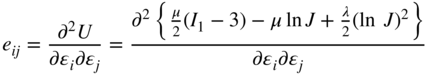
The fourth-order Lagrangian tensor of the elastic coefficients for the Neo–Hookean material can be obtained by differentiating the expression for the second Piola–Kirchhoff stress tensor with respect to the components of the Green–Lagrange strain tensor. That is,

Note that ∂(σP2)ij/∂ϵkl = (∂(σP2)ij/∂ckl) (∂ckl/∂ϵkl), and (∂ckl/∂ϵkl) = 2, where ckl here is the kl th element of the right Cauchy–Green deformation tensor Cr. The preceding equation can be used to define the fourth-order tensor of elastic coefficients as

In this equation,
are the effective coefficients for the Neo–Hookean material. It is clear from Equation 51 that the elastic coefficients of the Neo-Hookean material model are not constants. These coefficients depend on the position vector gradients, which are functions of the continuum displacements. While the material is still considered homogeneous because it has the same properties (![]() and
and ![]() ) in the reference configuration, the elastic coefficients
) in the reference configuration, the elastic coefficients ![]() will have values that depend on the location of the material points as it is clear from Equation 51, which shows the dependency on the right Cauchy–Green deformation tensor
will have values that depend on the location of the material points as it is clear from Equation 51, which shows the dependency on the right Cauchy–Green deformation tensor ![]() .
.
Alternatively, one can obtain the elastic coefficients eij used in the vector and matrix notation instead of the tensor notation using the following equation:
The special case of nearly incompressible material can be obtained from the general Neo–Hookean model by choosing Lame's constants such that ![]() . In this case, the third term in the strain energy density function λ (ln J)2/2 can be considered as a penalty term, which makes the deviation of J from 1 very small, and as a consequence, enforces the incompressibility condition.
. In this case, the third term in the strain energy density function λ (ln J)2/2 can be considered as a penalty term, which makes the deviation of J from 1 very small, and as a consequence, enforces the incompressibility condition.
Incompressible Mooney–Rivlin Materials
A general form of the strain energy function for incompressible rubber materials is based on Mooney–Rivlin model. For incompressible materials, J = det(J) = 1, and therefore, the third invariant of Cr is equal to one because I3 = det(Cr) = J2 = 1, Therefore, the strain energy function for such incompressible materials depends on I1 and I2 only and is given by (Bonet and Wood, 1997)

In this equation, the coefficients μrs are constants. A special case of the preceding equation that was shown to match experimental results by Mooney and Rivlin is when μ01 and μ10 only are different from zero. In this particular case, one has
The incompressibility condition that J = 1, or equivalently I3 = 1, must be imposed. In order to impose this constraint, one can use the technique of Lagrange multipliers or the penalty method. The method of Lagrange multipliers introduces additional algebraic equations and unknown constraint forces, which enter into the formulation of the dynamic equations (Roberson and Schwertassek, 1988; Shabana, 2013). If the dependent variables that result from introducing the algebraic equations are not systematically eliminated, one must solve a system of differential and algebraic equations. The use of Lagrange multipliers requires a more sophisticated numerical procedure in order to be able to accurately solve the resulting dynamic equations.
On the other hand, if the penalty method is used, the preceding equation for the strain energy density function can be modified to include the penalty terms. There are several forms that can be used to introduce a penalty energy function Up. One example is to use an energy function that produces a restoring force if the determinant of the matrix of position vector gradients deviates from one. In this case, the penalty function takes the form Up = k(J − 1)2/2, where k is a stiffness coefficient that must be selected high enough to enforce the incompressibility condition. In this case, the modified strain energy density function can be written as Ū = U + Up. Another example is to use the following modified strain energy density function (Belytschko et al., 2000).

In this equation, Up = k1 ln I3 + k2(ln I3)2 is the penalty energy term, and k1 and k2 are constants. The constant k1 is selected such that the components of the second Piola–Kirchhoff stress tensor are zero in the initial configuration. This condition is satisfied if k1 = − (μ10 + 2 μ01) (Belytschko et al., 2000). The penalty constant k2 must be chosen large enough such that the compressibility error is small. The value of such constant must not be selected extremely large in order to avoid numerical problems associated with high-stiffness coefficients. The value recommended by Belytschko et al. (2000) is k2 = 103 × max(μ01, μ10) to k2 = 107 × max(μ01, μ10). The components of the second Piola–Kirchhoff stress tensor can be obtained from the modified strain energy density function as

The penalty method has two main drawbacks. First, it requires making assumptions for the penalty coefficients because there is no standard formula for determining these coefficients. Second, if the penalty coefficients required to satisfy the incompressibility condition are very high, the system becomes very stiff and numerical problems can be encountered as previously discussed. On the other hand, although the use of Lagrange multipliers leads to a more sound analytical approach, one must develop a procedure for solving the resulting differential and algebraic equations, as previously mentioned. The algebraic constraint equations reduce the number of the system degrees of freedom and lead to a more robust, yet more complex numerical algorithm. The use of the penalty method, on the other hand, does not require introducing algebraic constraint equations.
Objectivity
In the literature, there are different constitutive models that are used to characterize the behavior of different materials. These constitutive models, however, must satisfy the objectivity requirement or the principle of material frame indifference. Any form of the constitutive equations leads to a functional relationship that can be written in the form σ = Φ(J). Using this functional relationship, one can, in a straightforward manner, obtain the conditions that must be met in order to satisfy the objectivity requirement. For example, consider σ to be the Cauchy stress tensor. If the continuum is subjected from its current configuration to a rigid-body rotation defined by the transformation matrix A, the new matrix of position vector gradients is defined as ![]() , whereas the new Cauchy stress tensor is defined as
, whereas the new Cauchy stress tensor is defined as ![]() . It follows that
. It follows that ![]() . That is, the constitutive equations must satisfy the condition Φ(AJ) = AΦ(J)AT in order to meet the objectivity requirement.
. That is, the constitutive equations must satisfy the condition Φ(AJ) = AΦ(J)AT in order to meet the objectivity requirement.
Recall that the second Piola–Kirchhoff stress tensor does not change under an arbitrary rigid-body rotation. If this stress tensor is used, the constitutive model can in general be written in the form σP2 = ΦP2 (J). In the case of a rigid-body rotation defined by the transformation matrix A, one has ![]() and
and ![]() . It follows that
. It follows that ![]() , which leads to the condition ΦP2(AJ) = ΦP2(J).
, which leads to the condition ΦP2(AJ) = ΦP2(J).
4.7 LINEAR VISCOELASTICITY
In this section, viscoelastic materials that are dissipative in nature are considered. Such materials, which are not hyperelastic, can have permanent deformation when the loads are released. The constitutive equations for viscoelastic models are written in terms of derivatives of strains or stresses. These constitutive equations, as will be demonstrated, can be given in the form of differential or integral equations. For this reason, unlike the case of purely elastic model, the full history of the strains and stresses is required. First, the case of one-dimensional linear viscoelastic models is discussed. Generalization of the one-dimensional theory to three-dimensional models is demonstrated next. In the case of linear viscoelasticity, one does not need to distinguish between different stress and strain measures because the linear theory is applicable, for the most part, to small-deformation problems.
One-Dimensional Model
Several models are used in the analysis of viscoelastic materials. First, the standard model shown in Figure 1 is considered. This model consists of two springs and a dashpot that are arranged as shown in the figure. The spring constants are Ep and Es and the dashpot constant is η. The total strain can be written as the sum of the elastic strain due to the deformation of the spring Es and the inelastic strain due to the motion of the dashpot (assumption of series connection), that is,
where ϵ is the total strain, ϵse is the elastic strain in the spring Es, and ϵv is the strain due to the viscosity of the material. Equation 58 is an example of the strain additive decomposition which can be assumed in the case of linear viscoelasticity. Differentiating the preceding equation with respect to time, one obtains

Figure 4.1 Standard model
Using the arrangement of the standard model and small strain assumptions, the stresses in the spring and the dashpot are assumed equal, that is
The total stress can then be written as
Equation 60 shows that
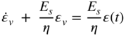
or

where τr = η/Es is called the relaxation time.
Equation 63 can be considered as a first-order nonhomogeneous ordinary differential equation in the strain ![]() . The solution of this equation can be obtained, as shown in Example 5, using the convolution or the Duhamel integral as (Weaver et al., 1990; Shabana, 1996c)
. The solution of this equation can be obtained, as shown in Example 5, using the convolution or the Duhamel integral as (Weaver et al., 1990; Shabana, 1996c)

where H(t − τ) is the impulse response function defined as
Integrating Equation 64 by parts and using the condition that ϵ(t) → 0 as t → − ∞, one obtains

Substituting this equation into the expression for the stress of Equation 61 in order to eliminate ϵv and writing ϵ in terms of the integral of ![]() , one obtains
, one obtains

where the kernel G(t) is called the relaxation function associated with the standard model and is defined as
Equation 67 is the constitutive equation in the case of one-dimensional linear viscoelastic material models. This equation is based on the assumptions of the standard model of viscoelasticity.
For the standard model, the stress response can be inverted to obtain an expression for the strain history in terms of the stress history using the following convolution integral:

where K is the creep function, which is defined for the standard model by the following equation:

In this equation,
It is important to point out that the use of the convolution integral as the solution of ordinary differential equations implies the use of the principle of superposition. Therefore, the convolution integral can only be used to obtain the solution of linear ordinary differential equations.
Other Viscoelastic Models
Although in this section, only the standard model is considered, it is important to mention that two other models are often used in the analysis of the viscoelastic behavior of materials. These are the Maxwell model and the Kelvin (Voigt) model (Fung, 1977). In the Maxwell model, only series connection is used, whereas the Voigt model has elements that are connected in parallel. Both models (Maxwell and Voigt) can be obtained as special cases of the standard model previously discussed in this section. The Maxwell model is a special case in which Ep = 0. It is important to note, however, that for the Maxwell model it is impossible to write the strain in terms of the stress because the creep function is not defined as it is clear from Equation 70. On the other hand, the Voigt model can be obtained from the standard model in case Es = 0. In this case, one has

For the Voigt model, one can obtain a convolution integral in which the history of the strain is written in terms of the history of the stress. The inverse representation in which the history of the stress is written in terms of the history of the strain cannot be defined for the Voigt model.
Generalization
The standard model can be generalized to include an arbitrary number of series spring–dashpot elements connected in parallel in addition to the spring Ep as shown in Figure 2. In this case, Equation 61 can be generalized and written as (Simo and Hughes, 1998)


Figure 4.2 Generalization
In this equation, N is the total number of spring-dashpot elements connected in parallel. One can define

and use this equation to write Equation 73 as

For each series connection, an equation similar to Equation 60 can be obtained. Therefore, the viscous strains ϵvi are governed by the following equations:

where τri = ηi/Esi. In this case, one can use a procedure similar to the one described previously in this section to obtain the following convolution integral for the stress:

with the relaxation function G(t) defined as

Note that Equation 77 is in the same form as Equation 67 with a different definition of the relaxation function.
Elastic Energy and Dissipation
The stored strain energy density function in the springs of the generalized standard model can be written as

Differentiation of this equation with respect to the strain yields

This equation shows that

Recall that
The energy dissipated, assuming a linear force–strain rate relationship, can be written as

This dissipated energy is greater than zero for positive viscous damping coefficients. It is clear that the viscous stress can be obtained from the energy dissipation function as

This equation bears a similarity to the equations used to define the elastic stresses in the case of hyperelastic materials. Here the dissipation function replaces the strain energy function.
Another Form of the Viscoelastic Equations
The elementary model discussed in this section can be presented in a different form, which can be extended in a straightforward manner to include nonlinear elastic response (Simo and Hughes, 1998). To this end, one can introduce a new set of stress-like variables called partial stresses:
It follows that

and

Let
Using the definition of Et, of Equation 74, one can show that the coefficient in the preceding equation must satisfy the following relationship:

Therefore, the first-order differential equations for the partial stresses can be written as

The solution of this equation must satisfy ![]() .
.
It is clear from Equation 86 that one can introduce an auxiliary strain energy density function Uv such that Uv = Etϵ2/2. Using this definition and Equation 86, the stress σ can be defined as ![]() . This form of the stress can be generalized and used in the case of the three-dimensional analysis.
. This form of the stress can be generalized and used in the case of the three-dimensional analysis.
Three-Dimensional Linear Viscoelasticity
The one-dimensional model discussed in this section can be further generalized to the case of three-dimensional analysis. If Uv is the strain energy density function, one can write the following model previously presented in this section (Simo and Hughes, 1998)

Viscoelastic constitutive models are often used for modeling the response of polymer materials. For these materials, the bulk response is elastic and appears to be much stiffer than the deviatoric response. For this reason, the assumption of incompressibility is often used. Using this assumption, the strain tensor can be written as
where ϵd is the deviatoric strain tensor and ϵt is the volumetric strain tensor, defined as
The stored strain energy density function can also be written as
In this equation, Ud and Ut, are, respectively, the strain energy density functions due to the deviatoric and volumetric strains. It can be shown that ∂Uv/∂ϵ in the definition of σ in Equation 91 can be written using chain rule of differentiation as

The evolution equations for the partial stresses can be written as

As in the one-dimensional theory, the material parameters must satisfy the following condition:

and the solutions for the partial stresses must satisfy ![]() . Using the convolution integrals, the solution for the partial stresses can be obtained as
. Using the convolution integrals, the solution for the partial stresses can be obtained as

Substituting this equation into the expression for σ, one obtains the constitutive equations in the convolution integral form as

In this equation,

The function G(t) is called the normalized relaxation function. Other forms of the relaxation function G(t) can also be considered. One can also consider the bulk response to be viscoelastic by simply making the following substitution in the convolution form of the constitutive equation:

where Gb(t) is a suitable relaxation function associated with the bulk response (Simo and Hughes, 1998). Note that if Ut is a linear function of ϵt, the term dev(∂Ut/∂ϵ) is the null tensor.
A Kelvin–Voigt model that distinguishes between the bulk and deviatoric responses can also be developed. For this model, one can write the following constitutive equations (Garcia-Vallejo et al., 2005):

In this equation, S and ϵd are, respectively, the deviatoric stress and strain tensors; Ed and Dd are, respectively, the tensors of elastic and damping coefficients; p is the hydrostatic pressure; ϵt is the dilatational strain; and Et and Dt are elastic and damping coefficients. In the case of linear elastic materials, Ed = 2μI and Et = 3 K, where μ is the shear modulus or modulus of rigidity, K = E/3(1 − 2γ) is the bulk modulus, E is the modulus of elasticity, and γ is the Poisson ratio. In the literature (Garcia-Vallejo et al., 2005), the damping coefficients are assumed to be Dd = 2μξd, Dd = 3Kξt where ξd and ξt are the dissipation coefficients associated with the deviatoric and volumetric strains. Using the preceding equation and the fact that σ = pI + S and ϵ = ϵtI + ϵd, the constitutive equations based on the Kelvin–Voigt model can be written as
In this equation, Dv, is an appropriate damping matrix.
4.8 NONLINEAR VISCOELASTICITY
In the case of the nonlinear analysis, the principle of superposition employed in the preceding section for the linear analysis does not apply. Furthermore, the infinitesimal strain tensor can no longer be used, appropriate strain and stress measures must be used, and the constitutive equations must be frame-indifferent in order to satisfy the objectivity requirement.
A straightforward generalization of the formulation presented in the preceding section to the case of finite strains is to use a multiplicative decomposition of the matrix of position vector gradients. To this end, one can define the following matrix:
Using this definition, one has the following simple multiplicative decomposition of J:
Because on the right-hand side of Equation 104, every row of J is multiplied by ![]() , it follows that the determinant of
, it follows that the determinant of ![]() is always equal to one, that is
is always equal to one, that is
One can then define the following right Cauchy–Green deformation tensors:
As was previously shown

The stored elastic energy can be written as the sum of two parts as follows:
In this equation, U1 is the strain energy due to the volumetric change, whereas U2 is the strain energy due to volume-preserving deformations.
Motivated by the development presented in the preceding section, the second Piola–Kirchhoff stress tensor can be defined for the viscoelastic model using the energy density function and the partial stresses as

In this equation, qi, i = 1, 2,…, N, are the partial stresses. Because σP2 does not change under an arbitrary rigid-body motion, as shown in the preceding chapter, the partial stresses qi must remain unchanged under the arbitrary rigid-body motion in order to satisfy the objectivity requirement for the stress. The evolution equations for the partial stresses can be written as
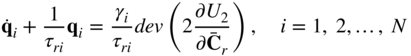
In this equation, the trace of ![]() is not in general equal to zero as in the case of the second Piola–Kirchhoff stress tensor. The material parameters must satisfy the following condition:
is not in general equal to zero as in the case of the second Piola–Kirchhoff stress tensor. The material parameters must satisfy the following condition:

The solutions for the partial stresses must satisfy ![]() . Equation 111 represents a set of N linear first-order differential equations, which can be solved for the partial stresses. Using the convolution integrals, the solution for the partial stresses can be obtained as
. Equation 111 represents a set of N linear first-order differential equations, which can be solved for the partial stresses. Using the convolution integrals, the solution for the partial stresses can be obtained as

Substituting this equation into the expression for σP2, one obtains the constitutive equations in the convolution integral form as (Simo and Hughes, 1998)

In this equation,

The function G(t) is the normalized relaxation function. As mentioned in the preceding section, other forms of the relaxation function G(t) can also be considered.
Another Model
Another formulation that is based on the Maxwell model and presented in Belytschko et al. (2000) is discussed in the remainder of this section. In this model, it is assumed that the second Piola–Kirchhoff stresses, in the case of the nonlinear viscoelastic model, are related to the Green–Lagrange strains using the following constitutive model:

where R is the tensor of relaxation functions. One form of the tensor R motivated by the model presented in the preceding section and is considered as a specialization to the generalized Maxwell model that consists of nv Maxwell elements connected in parallel is in terms of Prony series given as

The hyperelastic model can be obtained using the constitutive model presented in this section by setting τrk equal to infinity. Note also that by differentiating the constitutive equation presented in this section, one obtains

where ![]() and (σP2)k are called the partial stresses. The preceding equation shows that the model presented in this section for nonlinear viscoelasticity can be considered as a series of parallel connections of Maxwell elements.
and (σP2)k are called the partial stresses. The preceding equation shows that the model presented in this section for nonlinear viscoelasticity can be considered as a series of parallel connections of Maxwell elements.
4.9 A SIMPLE VISCOELASTIC MODEL FOR ISOTROPIC MATERIALS
In this section, a simple viscoelastic model for isotropic materials is presented. In this model, for simplicity, the viscoelastic response is restricted to the deviatoric stress and strains, whereas the volume change is assumed to obey linearly elastic relationship. Recall the following form of the Cauchy stress tensor developed in the preceding chapter:
where S is the stress deviator tensor and p is the hydrostatic pressure defined as

Note that tr(S) = 0, and because Cauchy stress tensor is used, the hydrostatic pressure p has a physical interpretation. As discussed in the preceding chapter, the decomposition of the Cauchy stress tensor to deviatoric and hydrostatic pressure parts can be used to obtain the following decomposition for the second Piola–Kirchhoff stress tensor:
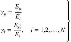
where
The tensor SP2 is the deviatoric components of the second Piola–Kirchhoff stress tensor. Recall that the trace of SP2 is not necessarily equal to zero despite the fact that the trace of S is equal to zero.
In a similar manner, the Green–Lagrange strain tensor can be written as follows:
where ϵd is the strain deviator tensor and ϵt is the dilatation. In the model presented in this section, the pressure–volume relationship is assumed to be linear and is defined as
where K is the bulk modulus. A more general model than the one presented in this section can be obtained by using, in the relationships developed in the remainder of this section, the components of the Green–Lagrange strain and the second Piola–Kirchhoff stress tensors instead of the deviatoric parts.
Constitutive equations that relate the stress and strain deviators and are based on the differential form and a generalized Maxwell model that consists of nv elements connected in series can be written as (Zienkiewicz and Taylor, 2000)

In this equation, G is a relaxation modulus, qk, k = 1, 2,…, nv, are dimensionless deviatoric partial strains, and μk are dimensionless parameters that satisfy the following condition:

The deviatoric partial strains are obtained by solving the following system of ordinary first-order differential equations:

in which τrk, k = 1,2,…, nv, are the relaxation times. If the state of strains is known at a given time, a simple single-step method can be used to solve the preceding equation for the partial deviatoric strains qk. The partial strains can then be substituted into the constitutive equations to determine the deviatoric stress tensor SP2. Because the hydrostatic pressure can be determined using the linear elastic model of Equation 124, one can obtain the elements of the second Piola–Kirchhoff stress tensor using Equation 121.
If the coefficients that appear in the equations presented in this section are nonlinear and depend on the state of stress and strain, an iterative Newton–Raphson algorithm can be used to solve for the stresses. In this case, the tangent moduli for the viscoelastic model must be determined. The tangent moduli for the viscoelastic isotropic material model discussed in this section can be found in the literature (Zienkiewicz and Taylor, 2000).
4.10 FLUID CONSTITUTIVE EQUATIONS
Unlike solids, fluids cannot resist shear stresses because any shear force applied to a fluid produces motion. In the case of fluids, the stress components are expressed as functions of the rate of strains. If the shear stresses are proportional to the rate of strains, one has the case of Newtonian viscous fluid. The constant of proportionality is the viscosity coefficient. If the effect of viscosity is neglected, one has the case of inviscid flow in which the effect of shear is neglected. In reality, no fluid has viscosity coefficient that is equal to zero. The viscosity coefficient can be a function of the spatial coordinates, pressure, and/or temperature. A flow is called incompressible if the density and volume are assumed to remain constant.
Linear constitutive equations of the fluid can be assumed in the following form (Spencer, 1980):
In this equation, ρ is the mass density, T is the temperature, D is the rate of deformation tensor, p is the hydrostatic pressure, and E is the fourth-order tensor of viscosity coefficients. The preceding equation states that in the case of fluid motion, all the stresses are linear functions of the components of the rate of deformation tensor. The normal stresses in particular are equal to the hydrostatic pressure plus terms that depend linearly on the components of the rate of deformation tensor.
If the fluid is assumed to be isotropic, one can use an argument similar to the one made in the case of solids to derive the fluid constitutive equations. In this case, one can write the following fluid constitutive equations (Spencer, 1980):
where λ and μ are viscosity coefficients that depend on the fluid density and temperature. These viscosity coefficients are different from Lame's constants previously introduced in this chapter. It is clear from the preceding equation that if the velocity gradients are equal to zero, the shear stresses are equal to zero, and the normal stress components reduce to the hydrostatic pressure p. In the preceding equation, μ is the coefficient of shear viscosity and (λ + (2 μ/3)) is called the coefficient of bulk viscosity. If λ + (2 μ/3) = 0, one has the Stokes' relation.
The relationship between the stress components and the rate of strains must be invariant under coordinate transformations. Recall that the rate of deformation tensor satisfies the objectivity requirement when it is used with a proper stress measure, which in this case is the Cauchy stress tensor σ, because σ : L = σ : D, as shown in the preceding chapter. Using this fact, one can show that the fluid constitutive equations presented in this section are invariant under an arbitrary rigid-body motion. It can be shown that isotropy follows from Equation 128 and the requirement that the stresses must be selected to satisfy the objectivity requirement. Therefore, one does not need to introduce the isotropy as a separate assumption (Spencer, 1980).
For incompressible fluids, tr(D) = 0. In this special case, the mass density ρ is constant and Equation 129 reduces to
In principle, as previously discussed, the incompressibility condition must be introduced using algebraic constraint equations imposed on the deformation in order to ensure that the volume remains unchanged throughout the fluid motion. The algebraic equations must be solved simultaneously with the dynamic equations of motion of the fluid. Introducing an incompressibility algebraic constraint equation, as previously mentioned, leads to a constraint force (stress reaction) that can be used to determine the hydrostatic pressure, which enters into the formulation of the constitutive equations. This constraint force can be expressed in terms of a Lagrange multiplier. Note that in the preceding equation the hydrostatic pressure and the viscosity coefficient depend only on the temperature T. A fluid that is incompressible and inviscid is called an ideal fluid. In this special case, there are no constitutive equations required and the stresses can be determined by simply using the equations σ = −pI.
4.11 NAVIER–STOKES EQUATIONS
In order to obtain the fluid equations of motion, the fluid constitutive equations can be used to define the stresses, which in turn can be substituted into the partial differential equations of equilibrium obtained in the preceding chapter. This leads to the well-known Navier–Stokes equations (White, 2003). In the case of incompressible fluid, the incompressibility algebraic equations must be added to the Navier–Stokes equations in order to ensure that the fluid volume remains unchanged. In the preceding chapter, it was shown that the dynamic equations of equilibrium in the case of a symmetric stress tensor are given by
where σ is the stress tensor, fb is the vector of the body forces, ρ is the mass density, and a is the vector of absolute acceleration of the material points. The variables in the preceding equation are defined in the current configuration. Using the definition of the stress given for isotropic materials by Equation 129, one can write
Substituting this equation into Equation 131, one obtains
If the fluid is assumed to be Newtonian, the preceding equation leads to
This equation is known as the Navier–Stokes equations.
For an incompressible fluid, tr(D) = 0, the preceding equation reduces to
The ratio α1 = μ/ρ is known as the kinematic viscosity. If the Stokes' relation is assumed, one has α1 + α2 = α1/3, where α1 = λ/ρ.
In order to solve the Navier–Stokes equations, the boundary conditions must be defined. In general, the viscous fluid is assumed to stick to the boundaries such that the fluid has the boundary velocities in the regions of contact. If the boundary is stationary, the viscous fluid is assumed to have zero velocity at the boundary. In the case of inviscid fluid, the fluid can have a tangential velocity at the boundary, whereas the normal component of the velocity is assumed to be zero.
PROBLEMS
-
1 Write explicitly all the conditions of the material symmetry that lead to Equation 22.
-
2 In the case of plane stress, σ33 = σ13 = σ23 = 0. Derive the constitutive equation in this plane stress case.
-
3 In the case of plane strains, ϵ33 = ϵ13 = ϵ23 = 0. Derive the constitutive equation in this case of plane strains.
-
4 Let I1, I2, and I3 be the invariants of the right Cauchy–Green strain tensor Cr. Show that ∂I1/∂Cr = I,
 .
. -
5 For the Neo–Hookean material model presented in this chapter, show that the second Piola–Kirchhoff stress tensor is given as
 , where λ and μ are Lame's constants and Cr is the right Cauchy–Green deformation tensor.
 -
6 For the Neo–Hookean material model presented in this chapter, show that the Kirchhoff stress tensor is given as
 , where λ and μ are Lame's constants and Cl is the left Cauchy–Green deformation tensor.
 -
7 Show that the fourth-order tensor of the elastic coefficients for the Neo–Hookean material model presented in this chapter is given as
 , where Cr is the right Cauchy–Green deformation tensor, and λh and μh are the coefficients defined in this chapter.
 -
8 Show that the creep function for the one-dimensional standard viscoelastic model is given by
 , where the coefficients that appear in this equation are defined in Section 7.
 -
9 Obtain the constitutive equations for the simple one-dimensional viscoelastic Maxwell model.
-
10 Derive a more general viscoelastic model for isotropic materials than the one presented in Section 9 by using, in the relationships developed in Section 9, the components of the Green–Lagrange strain and the second Piola–Kirchhoff stress tensors instead of their deviatoric parts.