CHAPTER 2
KINEMATICS
In this chapter, the general kinematic equations for the continuum are developed. The kinematic analysis presented in this chapter is purely geometric and does not involve any force analysis. The continuum is assumed to undergo an arbitrary displacement and no simplifying assumptions are made except when special cases are discussed. Recall that in the special case of an unconstrained three-dimensional rigid-body motion, six independent coordinates are required in order to describe arbitrary rigid-body translation and rotation displacements. The general displacement of an infinitesimal material volume on a deformable body, on the other hand, can be described in terms of 12 independent variables: 3 translation parameters, 3 rigid-body rotation parameters, and 6 deformation parameters. One can visualize these modes of displacements by considering an infinitesimal cube that may undergo an arbitrary displacement. The cube can be translated in three independent orthogonal directions (translation degrees of freedom), rotated as a rigid body about three orthogonal axes, and subjected to six independent modes of deformation. These deformation modes are elongations or contractions in three different directions and three shear deformation modes.
It is shown in this chapter that the rotations and the deformations can be completely described using the matrix of the position vector gradients, which in general has nine independent elements. This fact can be mathematically proven using the polar decomposition theorem discussed in the preceding chapter. The deformation at the material points on the body can be described in terms of six independent strain components. These strain components can be defined in the undeformed reference configuration leading to the Green–Lagrange strains or can be defined using the current deformed configuration leading to the Eulerian or Almansi strains. The velocity gradients and the rate of deformation tensor also play a fundamental role in the theory of nonlinear continuum mechanics and for this reason they are discussed in detail in this chapter.
The concept of objectivity or frame indifference, which is important in the analysis of large deformations, particularly in formulations that involve the strain rates, is also introduced and will be discussed in more detail in the following chapter. In order to correctly formulate the dynamic equations of the continuum, one needs to develop the relationships between the volume and area of the body in the reference configuration and its volume and area in the current configuration. These relationships as well as the continuity equation derived from the conservation of mass are presented in Sections 8 and 9. Reynolds' transport theorem, which is used in fluid mechanics, is discussed in Section 10. In Section 11, several examples of simple deformations are presented.
Whereas a continuum has an infinite number of degrees of freedom, for simplicity, concepts and definitions are explained in the examples throughout this book using models that have a finite number of degrees of freedom. This provides the reader with a natural introduction to the finite element formulations that will be discussed in later chapters.
2.1 MOTION DESCRIPTION
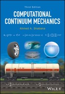
Figure 1 shows a body in the reference and current configurations. The position vector of an arbitrary material point on the body in the reference configuration is defined by the vector x = [x1 x2 x3]T, whereas the position vector of this arbitrary material point in the current configuration after displacement is defined by the vector r = [r1 r2 r3]T. One can then write the following relationship:
where u = [u1 u2 u3]T is the displacement vector, and the three vectors r, x, and u are defined in the same global coordinate system as shown in Figure 1. In the preceding equation, it is assumed that both the position and displacement vectors r and u are functions of the components of the position vector x in the reference configuration. That is, given a material point defined by the position x in the reference configuration, one should be able to define the position vector r of this point in the current configuration as well as the displacement vector u. In general, the position vector r and the displacement vector u can be written as functions of x and time t, that is
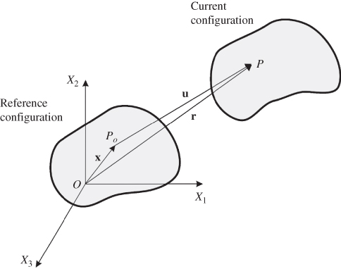
Figure 2.1 Reference and current configurations
The coordinates x are called the material or Lagrangian coordinates, whereas the coordinates r are called the spatial or Eulerian coordinates. Both sets of coordinates can be used in the formulation of the kinematic and dynamic equations. If the Lagrangian coordinates are used to formulate the dynamic equations, one obtains the Lagrangian description, which is often used in solid mechanics. If the Eulerian coordinates are used, on the other hand, one obtains the Eulerian description, which is often used in the study of the motion of the fluids. In the case of a fluid, it is sometimes inconvenient to describe the motion with respect to the reference configuration, as in the case of a flow around an airfoil. In the case of solids, on the other hand, the history of the deformation is important, and for this reason, the Lagrangian description is more suited.
Line Elements
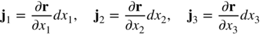
In the study of deformation, the change of the length of a line element is used to define the basic strain variables used in continuum mechanics. It is clear that if the change of the distance between two arbitrary points as the result of deformation is known, changes of areas and volumes can be determined. A differential line element dr in the current configuration can be written as
where J is the matrix of position vector gradients, also called the Jacobian matrix. This matrix is defined as follows:

In this equation, ![]() , i = 1, 2, 3. If there are no displacements of the particles of the body, the vector dr is equal to the vector dx. In this case, J is the identity matrix and has a positive determinant that is equal to one. Because the Jacobian matrix J cannot be singular and the displacement is assumed to be continuous function, the determinant of J must be positive. Therefore, a necessary and sufficient condition for a continuous displacement to be physically possible is that the determinant of J be greater than zero, that is, J is always positive definite. This requirement of continuous displacement allows transformation from the current configuration to the reference configuration and vice versa. It is therefore assumed that the transformation is one-to-one and the function r = r(x, t) is single-valued, continuous, and has the following unique inverse:
, i = 1, 2, 3. If there are no displacements of the particles of the body, the vector dr is equal to the vector dx. In this case, J is the identity matrix and has a positive determinant that is equal to one. Because the Jacobian matrix J cannot be singular and the displacement is assumed to be continuous function, the determinant of J must be positive. Therefore, a necessary and sufficient condition for a continuous displacement to be physically possible is that the determinant of J be greater than zero, that is, J is always positive definite. This requirement of continuous displacement allows transformation from the current configuration to the reference configuration and vice versa. It is therefore assumed that the transformation is one-to-one and the function r = r(x, t) is single-valued, continuous, and has the following unique inverse:
This property, when guaranteed for every material point on the body, allows for the transformation between the Eulerian and Lagrangian descriptions.
Rigid-Body Motion
Recall that in the special case of rigid-body motion, the length of a line segment remains constant. This implies that
In this special case of rigid-body motion, one has JTJ = JJT = I. That is, J is an orthogonal matrix that describes the relationship between the line element dx before the displacement and the line element dr after the displacement. Equation 9 shows that in the case of rigid-body motion, the stretch of the line element defined as |dr|–|dx| is equal to zero everywhere. Because the components of the line elements are not affected by the translation, the matrix J in the case of rigid-body motion describes pure rotation, and it is the matrix that can be used to define the orientation of the rigid body in space. In this special case of rigid-body motion, the elements of the Jacobian matrix J are the direction cosines of unit vectors that define the axes of a selected body coordinate system whose origin is attached to the rigid body (Goldstein, 1950; Greenwood, 1988; Shabana, 2013).
In the case of a rigid-body motion, as shown in Figure 3, one can always select a body coordinate system, ![]() , that moves with the body. Line segments or locations of the material points can be measured with respect to the origin of the body coordinate system. Without any loss of generality, one can assume that before displacement, the axes of the body coordinate system
, that moves with the body. Line segments or locations of the material points can be measured with respect to the origin of the body coordinate system. Without any loss of generality, one can assume that before displacement, the axes of the body coordinate system ![]() coincide with the axes of the global coordinate system X1X2X3. In this case, the location of an arbitrary material point on the rigid body can be defined after the displacement using the following equation:
coincide with the axes of the global coordinate system X1X2X3. In this case, the location of an arbitrary material point on the rigid body can be defined after the displacement using the following equation:
where rO is the vector that defines the location of the origin of the body coordinate system; J, in this case of a rigid-body motion, is an orthogonal matrix that can be expressed in terms of three independent orientation coordinates (Goldstein, 1950; Greenwood, 1988; Shabana, 2013); and xb is the vector that defines the position of the material points in the moving coordinate system. Note that if an assumption is made that the moving reference coordinate system coincides with the global coordinate system before displacement, one has x = xb.

Figure 2.3 Rigid-body motion
Floating Frame of Reference (FFR)
In this book, two different, yet equivalent, motion descriptions are frequently used to define the absolute position vector r. In the first motion description, the vector r is defined using absolute coordinates based on a description similar to the one used in Equation 3. In the second motion description, a coordinate system that follows the motion of the body is introduced. The position vector r can be defined in terms of the motion of this reference plus the motion of the body with respect to the reference. This description is referred to in this book as the floating frame of reference (FFR) approach. It is important to recognize that these two different descriptions are equivalent and are consistent with the general continuum mechanics description. That is, the FFR approach does not lead to a separation between the rigid-body motion and the elastic deformation. Whereas the reference motion is a rigid-body motion, this motion is not the rigid-body motion of the continuum because different references can be selected for the same continuum.
In the case of general displacement, the floating frame of reference follows the motion of the body but does not have to be rigidly attached to a point on the body. Nonetheless, it is required that there is no relative rigid-body displacement between the body and its coordinate system. Using the FFR formulation kinematic description, the global position vector of an arbitrary point, as shown in Fig. 4, can in general be written as ![]() , where
, where ![]() is the transformation matrix that defines the orientation of the body coordinate system, and
is the transformation matrix that defines the orientation of the body coordinate system, and ![]() measures the deformation of the body with respect to the selected body reference. Since the choice of
measures the deformation of the body with respect to the selected body reference. Since the choice of ![]() is arbitrary; one can have infinite number of arrangements for the body coordinate system, and consequently infinite ways for measuring the deformation. Because the deformation is considered a relative measure, strains are used to describe the body kinematics when developing a general continuum mechanics theory. While coordinate systems are imaginary, strains are defined using the gradients of position vectors, which have a clear physical meaning. Nonetheless, the relationship
is arbitrary; one can have infinite number of arrangements for the body coordinate system, and consequently infinite ways for measuring the deformation. Because the deformation is considered a relative measure, strains are used to describe the body kinematics when developing a general continuum mechanics theory. While coordinate systems are imaginary, strains are defined using the gradients of position vectors, which have a clear physical meaning. Nonetheless, the relationship ![]() is general, does not imply any approximation, and is the starting point in the development of the FFR formulation discussed in Chapter 6. This formulation is widely used in the multibody system (MBS) dynamics literature and allows for obtaining an efficient formulation for flexible bodies that undergo large rigid-body displacements as well as deformations that can be described using simple shapes. The FFR formulation was introduced many decades before the finite element (FE) method was introduced. The corotational frame used in the FE literature is not in general equivalent to the floating frame used in MBS dynamics. The configuration of the corotational frame is defined by the FE nodal coordinates, while the configuration of the floating frame is defined by a set of absolute Cartesian coordinates. If the FE nodal coordinates cannot correctly describe finite rigid-body displacements, as in the case of conventional beam, plate and shell elements that employ infinitesimal rotations as nodal coordinates; the corotational frame does not lead to zero strains under an arbitrary rigid-body displacement. On the other hand, the FFR formulation always leads to zero strains under an arbitrary rigid-body displacement regardless of the finite element used to describe the deformation. Furthermore, using the FFR kinematic description
is general, does not imply any approximation, and is the starting point in the development of the FFR formulation discussed in Chapter 6. This formulation is widely used in the multibody system (MBS) dynamics literature and allows for obtaining an efficient formulation for flexible bodies that undergo large rigid-body displacements as well as deformations that can be described using simple shapes. The FFR formulation was introduced many decades before the finite element (FE) method was introduced. The corotational frame used in the FE literature is not in general equivalent to the floating frame used in MBS dynamics. The configuration of the corotational frame is defined by the FE nodal coordinates, while the configuration of the floating frame is defined by a set of absolute Cartesian coordinates. If the FE nodal coordinates cannot correctly describe finite rigid-body displacements, as in the case of conventional beam, plate and shell elements that employ infinitesimal rotations as nodal coordinates; the corotational frame does not lead to zero strains under an arbitrary rigid-body displacement. On the other hand, the FFR formulation always leads to zero strains under an arbitrary rigid-body displacement regardless of the finite element used to describe the deformation. Furthermore, using the FFR kinematic description ![]() , one can show that the matrix of position vector gradients
, one can show that the matrix of position vector gradients ![]() can always be written as
can always be written as ![]() , where
, where ![]() is the identity matrix.
is the identity matrix.
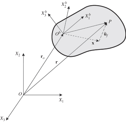
Figure 2.4 Floating frame of reference
The basic kinematic description used in the FFR formulation is based on the general kinematic equations used in the nonlinear continuum mechanics. Nonetheless, it is not necessary in computational continuum mechanics to write the displacement as the sum of reference motion plus the displacement with respect to the reference coordinate system. One can always use the expression r = r(x) with a proper definition of r in terms of x to correctly describe the general displacement of the continuum, as discussed in Chapter 5. This fact is also demonstrated by the following simple example.
Displacement Vector Gradients
As previously mentioned, in the case of general displacement, J is not an orthogonal matrix because the lengths of the line segments do not remain constant. There are, however, motion types in which the determinant of J remains constant, but J is not an orthogonal matrix. As will be shown later in this book, the determinant of J remains constant if the volume does not change as in the case of incompressible materials. This type of motion is called isochoric. Rigid-body motion is a special case of isochoric motion.
In the case of general displacement, the matrix of position vector gradients can also be written in terms of the displacement gradients by writing dr using Equation 1 as follows:
where Jd = (J − I) is the matrix of the displacement vector gradients defined as
In the analysis presented in this book, it is important to distinguish between the matrix of the position vector gradients and the matrix of the displacement vector gradients.
2.2 STRAIN COMPONENTS
The strain components defined in this section arise naturally when the equations of motion are formulated as will be shown in later chapters of this book. The strain components can be introduced by considering the elongation of a line element. The square of the length of the line element in the reference configuration is defined as
The square of the length of the line element in the current configuration can be defined using Equation 6 as
One measure of the elongation of the line element can be written using the preceding two equations as
which can be written as
where ϵ is the symmetric Green–Lagrange strain tensor defined as
Using the definition of the matrix of position vector gradients, the Green–Lagrange strain tensor ϵ can be written more explicitly as follows:

One can also write the Green–Lagrange strain tensor ϵ in terms of the elements of the matrix of the displacement vector gradients Jd. Recall that J = Jd + I and substituting in the definition of ϵ, one obtains the following definition of the elements of the strain tensor:

In this equation, ϵij are the elements of the tensor ϵ and ui,j = ∂ui/∂xj; i, j = 1, 2, 3. It is clear from the preceding two equations that the Green–Lagrange strains are nonlinear functions of the position vector and displacement vector gradients.
Because the strain tensor is symmetric, one can identify six independent strain components that can be used to define the following strain vector:
In this vector, ϵij for i = j are called normal strains and ϵij for i ≠ j are called the shear strains.
In the case of rigid-body motion, J is an orthogonal matrix, and as a consequence, ϵ = 0. This demonstrates that ϵ can be used as a measure of the deformation, whereas J cannot be used as deformation measure because it changes under an arbitrary rigid-body motion. In the case of rigid-body motion, the strains are identically zero. It is left to the reader as an exercise to show that if the nonlinear displacement gradient terms in Equation 19 are neglected, the Green–Lagrange strain tensor will not lead to zero strains under an arbitrary rigid-body motion.
Geometric Interpretation of the Strains
The gradient vectors ![]() , define the rate of change of the position vector r with respect to the coordinate xi. Therefore, the normal strains,
, define the rate of change of the position vector r with respect to the coordinate xi. Therefore, the normal strains, ![]() , measure the change of the length of the gradient vectors. On the other hand, the shear strains,
, measure the change of the length of the gradient vectors. On the other hand, the shear strains, ![]() , i ≠ j measure the change of the relative orientation between the gradient vectors.
, i ≠ j measure the change of the relative orientation between the gradient vectors.
Another geometric interpretation of the strains can be provided for simple cases. To this end, the extension of the line element per unit length can be defined as

This equation defines what is called engineering strain because the extension is divided by the length in the reference configuration. Another measure that can be used is the logarithmic or natural strain defined as ![]() . Equation 21 leads to
. Equation 21 leads to
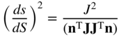
Using Equations 16 and 22, one can write the following quadratic equation for the strain ϵ:
where α = 2tTϵt, and t = dx /l0. Equation 23, which is a quadratic equation, has two solutions, ![]() . The second solution is not physically possible because it does not represent a rigid-body motion. Therefore, the strain ϵ can be evaluated using the components of the Green–Lagrange strain tensor as
. The second solution is not physically possible because it does not represent a rigid-body motion. Therefore, the strain ϵ can be evaluated using the components of the Green–Lagrange strain tensor as
This equation can be used to provide a measure of the elongation of a line element.
Consider the special case in which dx = [dx1 0 0]T; one obtains in this special case from the definition of the Green–Lagrange strain tensor, the following equation:
Using this equation, one has ![]() , or
, or ![]() . In the case of small strains, it can be shown that
. In the case of small strains, it can be shown that ![]() . Because shear strains can be defined using the dot product of vectors, these strains can always be defined in terms of angles or rotations. Therefore, a geometric interpretation of the shear strains can also be obtained.
. Because shear strains can be defined using the dot product of vectors, these strains can always be defined in terms of angles or rotations. Therefore, a geometric interpretation of the shear strains can also be obtained.
Eulerian Strain Tensor
Because dx can be written as
one can write
Using this equation, the Eulerian or Almansi strain tensor is defined as
This tensor is also a symmetric tensor. It is important to note that the components of the Eulerian (Almansi) strain tensor are defined using the current configuration, whereas the components of the Green–Lagrange strain tensor are defined using the reference configuration. Such definitions are important when the expressions of the elastic forces due to deformation are developed. Clearly, the relationship between the Green–Lagrange strain tensor and the Eulerian strain tensor can be written as
This equation can be interpreted as ϵ is the pullback of ϵe by J, or ϵe is the push-forward, of ϵ in the equation ![]() . In the case of infinitesimal strains, the Eulerian strain tensor is called Cauchy strain tensor. One can show that in the case of infinitesimal strains (small displacement gradients), one has
. In the case of infinitesimal strains, the Eulerian strain tensor is called Cauchy strain tensor. One can show that in the case of infinitesimal strains (small displacement gradients), one has
That is, the Eulerian and Lagrangian strain tensors are equal in the case of infinitesimal strains.
2.3 OTHER DEFORMATION MEASURES
Other deformation measures that are invariant under an arbitrary rigid-body motion can be used as alternatives to the Lagrangian and Eulerian strain tensors. In this section, some of these deformation measures are defined.
Right and Left Cauchy–Green Deformation Tensors
In order to introduce alternate strain measures, a unit vector t is defined as
Using this definition, one can write

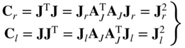
where Cr is a symmetric tensor called the right Cauchy–Green deformation tensor and is defined as
This tensor can be used as a measure of the deformation because in the case of an arbitrary rigid-body displacement Cr = I, and it remains constant throughout the rigid-body motion. The Green–Lagrange strain tensor can be expressed in terms of Cr as
That is, the tensors Cr and ϵ have a linear relationship. It follows that the derivatives of one tensor with respect to a set of coordinates can be used to define the derivatives of the other tensor with respect to the same coordinates. This linear relationship can be conveniently used when different constitutive models are used. Some of these constitutive models are expressed in terms of ϵ, whereas the others are expressed in terms of Cr.
Another deformation measure is the left Cauchy–Green deformation tensor Cl defined as
This tensor also remains constant and is equal to the identity matrix in the case of rigid-body motion. The Eulerian strain tensor can be written in terms of Cl as
Infinitesimal Strain Tensor
It was previously mentioned that in the case of small strains, the Lagrangian and Eulerian strain tensors are the same and both are defined by the equation ![]() . In this equation, Jd is the matrix of displacement vector gradients. It is important, however, to point out at this point that the infinitesimal strain tensor is not an exact measure of the deformation because it does not remain constant in the case of an arbitrary rigid-body motion. Recall that in the case of a rigid-body motion
. In this equation, Jd is the matrix of displacement vector gradients. It is important, however, to point out at this point that the infinitesimal strain tensor is not an exact measure of the deformation because it does not remain constant in the case of an arbitrary rigid-body motion. Recall that in the case of a rigid-body motion ![]() is an orthogonal matrix. It follows that in the case of infinitesimal strains,
is an orthogonal matrix. It follows that in the case of infinitesimal strains,
This equation shows that the linear form of the strain tensors does not remain constant under an arbitrary rigid-body motion because J changes, as previously discussed. In order to provide an estimate of the errors as the result of using the infinitesimal strain tensor in the case of general rigid-body motion, we use the expression of the rotation matrix defined by Rodriguez formula. In the case of a rigid-body motion, J is the rotation matrix that can be defined using Rodriguez formula as follows:
where ã is the skew-symmetric matrix associated with a unit vector a along the axis of rotation and θ is the angle of rotation (Shabana, 2013). Substituting the preceding equation into the expression of the infinitesimal strain tensor and considering the fact that ã is a skew-symmetric matrix and (ã)2 is a symmetric matrix, one has
Because the components of the unit vector a can be equal to or less than one, the preceding equation shows that in the case of infinitesimal rotations, the error in the infinitesimal strain tensor is of second order in the rotation θ.
2.4 DECOMPOSITION OF DISPLACEMENT
Using the polar decomposition theorem discussed in Chapter 1, any nonsingular square matrix can be written as the product of two matrices; one is an orthogonal matrix, whereas the other is a symmetric matrix. Applying this decomposition to the matrix of position vector gradients J, one obtains
where AJ is an orthogonal rotation matrix, and Jr and Jl are symmetric positive definite matrices called, respectively, the right stretch and left stretch tensors. It follows from the preceding equation that
The right and left Cauchy–Green strain tensors Cr and Cl can be expressed, respectively, in terms of Jr and Jl as follows:
Therefore, Cr is equivalent to Jr, whereas Cl is equivalent to Jl. It is, however, easier and more efficient to calculate Cr and Cl for a given J than to evaluate Jr and Jl from the polar decomposition theorem.
Equation 42 shows that the deformation measures Cr and Cl do not depend on the orthogonal matrix AJ. The expression of Cr in the preceding equation with Equation 34 also shows that the Green–Lagrange strain tensor ϵ does not depend on the orthogonal matrix AJ because it can be written as ![]() . Similarly, the Eulerian strain tensor of Equation 36 can be written as
. Similarly, the Eulerian strain tensor of Equation 36 can be written as ![]() .
.
Homogeneous Motion
In the special case of homogeneous motion, the matrix of position vector gradients J is assumed to be independent of the coordinates x. In this special case, one can write r = Jx. The motion of the body from the initial configuration x to the final configuration r can be viewed as two successive homogeneous motions. In the first motion, the coordinate vector x changes to xi, and in the second motion, the coordinate vector xi changes to r. These two displacements can be described using the two equations xi = Jrx, and r = AJxi. Clearly, these two equations lead to r = AJxi = AJJrx = Jx. Therefore, any homogeneous displacement can be decomposed into a deformation described by the tensor Jr followed by a rotation described by the orthogonal tensor AJ. Similarly, if Jl is used instead of Jr, the displacement of the body can be considered as a rotation described by the orthogonal tensor AJ followed by a deformation defined by the tensor Jl.
Nonhomogeneous Motion
In the case of nonhomogeneous motion, the relationship between the coordinates can be written as dr = Jdx. Although J in this case is a function of the reference coordinates x, the polar decomposition theorem can still be applied. Different material points in this case have different decompositions and different stretch and rotation tensors.
2.5 VELOCITY AND ACCELERATION
The absolute velocity vector can be obtained by differentiation of r = r(x, t) with respect to time. This leads to
In developing this equation for the velocity, the vector x is assumed to be independent of time because it defines the position of the material points in the reference configuration. In fluid mechanics, the curl of the velocity given by ![]() is called the vorticity. In this definition,
is called the vorticity. In this definition, ![]() = [∂/∂r1 ∂/∂r2 ∂/∂r3]T. In the case of irrotational flow, the vorticity is equal to zero everywhere.
= [∂/∂r1 ∂/∂r2 ∂/∂r3]T. In the case of irrotational flow, the vorticity is equal to zero everywhere.
The absolute acceleration vector a(x, t) is the rate of change of the velocity of the material points with respect to time. The acceleration vector can then be written as

In deriving this equation, it is assumed again that the vector x is not a function of time.
As previously mentioned in this chapter, one can, without any loss of generality, select a coordinate system, the floating frame of reference, that follows the motion of the body. In this case, the position of an arbitrary point on the body is described by the global position of the origin of the floating frame plus the position of the arbitrary point with respect to the floating frame. In this case, as previously explained, the global position of a point on the body can be written as r = rO(t) + A(x + ūf(x, t)), where rO(t) is the global position of the body reference, A is the orthogonal transformation matrix that defines the orientation of the body coordinate system in the global system, and ūf (x, t) is the vector of deformation with respect to the body coordinate system. Differentiating the vector r once and twice with respect to time, one obtains, respectively, the absolute velocity and acceleration vectors of the arbitrary point. Using this motion description, the velocity and acceleration vectors include terms that represent the rate of change of the motion of the arbitrary point with respect to the origin of the floating frame. These terms include the Coriolis acceleration, as discussed in more detail in Chapter 6.
Eulerian Description
The velocity vector can also be expressed in terms of the spatial (Eulerian) coordinates as v = v(r, t). In this case, r is a function of time. The total derivative of this expression of the velocity is given by
The term (∂v/∂r)v is called the convective or transport term, while ∂v/∂t is called the spatial time derivative. The preceding equation can also be written as
where L is called the velocity gradient tensor and is defined as
Note that the velocity gradient tensor is obtained by differentiation with respect to the spatial coordinates.
Rate of Deformation and Spin Tensors
Another strain measure considered in this section is called the rate of deformation tensor. The rate of deformation tensor D, which is also called the velocity strain and is used in the formulation of some material constitutive laws, differs from Green–Lagrange strain tensor, which is a measure of the deformation and not the rate of deformation. In order to define the rate of deformation tensor, the velocity gradient tensor is written as the sum of a symmetric tensor and a skew-symmetric tensor as follows:
The first matrix on the right-hand side of this equation is symmetric and is called the rate of deformation tensor D, whereas the second matrix is a skew-symmetric matrix called the spin tensor W. The preceding equation can then be written as
where
The rate of deformation tensor D can be used as a measure of the deformation because it vanishes in the case of a rigid-body motion. In order to demonstrate this fact, the rate of change of the square of the length of the line segment is considered. This change can be written as
Using the definition of the matrix of the velocity gradients in terms of the rate of deformation and spin tensors, one obtains
Because W is a skew-symmetric matrix, drTWdr = 0, and as a result, the preceding equation reduces to
Because dr is arbitrary, the preceding equation shows that in the case of rigid-body motion the rate of deformation tensor D is identically zero and such a tensor can indeed be used as a measure of the rate of deformation. The preceding equation also shows that
where tc = dr/ld defines a unit vector.
Rate of Change of the Green–Lagrange Strain
A relationship between the rate of deformation tensor and the rate of change of the Green–Lagrange strain tensor can be obtained. To obtain this relationship, the tensor of velocity vector gradients is written as
Using this equation, the rate of deformation tensor can be written as
Differentiation of the Green–Lagrange strain tensor leads to
The preceding two equations show that
This equation is another example of a pullback operation in which a tensor associated with the undeformed configuration is defined using a tensor associated with the deformed or current configuration. The preceding equation also leads to ![]() , which is an example of a push-forward operation in which a tensor in the deformed (current) configuration is obtained using a tensor associated with the undeformed (reference) configuration. Here, the push-forward operation is simply the result of pushing forward the Lagrangian vector dx to the Eulerian vector dr using the Jacobian matrix J as shown in Equation 6. On the other hand, the pullback of the Eulerian vector dr to the reference configuration using J−1 defines the Lagrangian vector dx as dx = J−1dr. The relationship between the rate of deformation tensor and the Green–Lagrange strain tensor is an example of the push-forward and pullback operations. Other examples are presented in the literature (Belytschko et al., 2000).
, which is an example of a push-forward operation in which a tensor in the deformed (current) configuration is obtained using a tensor associated with the undeformed (reference) configuration. Here, the push-forward operation is simply the result of pushing forward the Lagrangian vector dx to the Eulerian vector dr using the Jacobian matrix J as shown in Equation 6. On the other hand, the pullback of the Eulerian vector dr to the reference configuration using J−1 defines the Lagrangian vector dx as dx = J−1dr. The relationship between the rate of deformation tensor and the Green–Lagrange strain tensor is an example of the push-forward and pullback operations. Other examples are presented in the literature (Belytschko et al., 2000).
Another way of defining the relationship between the rate of deformation tensor and the rate of change of the Green–Lagrange strain tensor is to use the function relationship between r and x. To this end, we write

Because
one has
as previously obtained. Note that ![]() and D are not related by orthogonal tensor transformation and, therefore, they do not represent the same physical variables. Furthermore, it is important to point out that the time integral of
and D are not related by orthogonal tensor transformation and, therefore, they do not represent the same physical variables. Furthermore, it is important to point out that the time integral of ![]() is path independent, whereas the time integral of D is path dependent. It is also important to keep in mind that the rate of deformation tensor is not the time derivative of the Eulerian (Almansi) strain tensor.
is path independent, whereas the time integral of D is path dependent. It is also important to keep in mind that the rate of deformation tensor is not the time derivative of the Eulerian (Almansi) strain tensor.
2.6 COORDINATE TRANSFORMATION
As discussed in Chapter 1, the gradients defined by differentiation with respect to a set of coordinates x1, x2, and x3 represent changes of the position vector along these coordinate lines. The rate of change of the position vector with respect to one set of coordinates differs from the rate of change of this vector with respect to another set of coordinates. Although the two sets of coordinates can be related by a transformation, the change of the set of coordinates does not change the coordinate system in which the position vector or the gradient vectors are defined. In fact, the gradient vectors obtained by differentiation of the vector r with respect to one set of coordinates can be written as a linear combination of the gradient vectors obtained by differentiation of r with respect to another set of coordinates, as discussed in Chapter 1. That is, the two sets of gradient vectors are defined in the same coordinate system. Nonetheless, the strain components defined by the two different sets of gradients give measures of deformations along two different sets of directions.
In one-dimensional problems, as in the case of Euler–Bernoulli beams, there is one gradient vector that defines the tangent to a space curve. Change of the scalar coordinate α used to define the gradient vector rα does not change the orientation of this tangent vector because any selected coordinate α differs from another coordinate β by a scalar multiplier. It follows that rα = rβ(∂β/∂α) which implies that rα and rβ are parallel vectors. In this case of a one-dimensional problem, ![]() will always define the strain along the tangent to the centerline of the beam regardless of what the coordinate α represents. Furthermore, this tangent remains defined in the same coordinate system in which the vector r is defined. In two-dimensional problems, as in the case of plates, change of the coordinates can lead to a change in the direction of the two resulting gradient vectors. Nonetheless, the two gradient vectors remain tangent to the surface at the point they are evaluated regardless of the coordinates used to define these gradient vectors. In the three-dimensional case, the change of coordinates can lead to a more general change in the orientation of the gradient vectors, as discussed in Chapter 1.
will always define the strain along the tangent to the centerline of the beam regardless of what the coordinate α represents. Furthermore, this tangent remains defined in the same coordinate system in which the vector r is defined. In two-dimensional problems, as in the case of plates, change of the coordinates can lead to a change in the direction of the two resulting gradient vectors. Nonetheless, the two gradient vectors remain tangent to the surface at the point they are evaluated regardless of the coordinates used to define these gradient vectors. In the three-dimensional case, the change of coordinates can lead to a more general change in the orientation of the gradient vectors, as discussed in Chapter 1.
In continuum mechanics, it is important to understand the rules that govern the coordinate (parameter) transformation because this transformation defines the coordinate lines along which the strain components are measured. In order to develop this transformation, we consider two sets of coordinates x = [x1x2x3]T and ![]() associated with two coordinate systems X1X2X3 and
associated with two coordinate systems X1X2X3 and ![]() , respectively. These two sets of coordinate lines are used for the same configuration of the continuum. The relationship between these two sets of coordinates can be written as
, respectively. These two sets of coordinate lines are used for the same configuration of the continuum. The relationship between these two sets of coordinates can be written as ![]() , where A is the transformation matrix that defines the relationship between the two sets of coordinate lines. The absolute position vector r can be written in terms of x or in terms of
, where A is the transformation matrix that defines the relationship between the two sets of coordinate lines. The absolute position vector r can be written in terms of x or in terms of ![]() . That is, r = r(x1 x2 x3) = r(
. That is, r = r(x1 x2 x3) = r(![]() ). The matrix of the position vector gradients (Jacobian matrix) can then be written by differentiation of the vector r with respect to x or with respect to
). The matrix of the position vector gradients (Jacobian matrix) can then be written by differentiation of the vector r with respect to x or with respect to ![]() . One can therefore write the following equation:
. One can therefore write the following equation:
That is, the gradients of the vectors r defined by differentiation with respect to coordinate lines along the axes of the coordinate system ![]() are defined as
are defined as
This rule of position vector gradient transformation is crucial in developing the finite element formulation presented in Chapter 5. Note that in the preceding equation, r is still the vector that defines the position vector of the material points, say in the X1X2X3 coordinate system. It follows that the columns of the matrices rx = ∂r/∂x and ![]() are vectors defined in the X1X2X3 coordinate system. In Chapter 5, finite elements that do not have a complete set of gradient vectors are considered. These finite elements are referred to as gradient deficient.
are vectors defined in the X1X2X3 coordinate system. In Chapter 5, finite elements that do not have a complete set of gradient vectors are considered. These finite elements are referred to as gradient deficient.
Strain Transformation
Using the gradient transformation developed in this section and the definition of the strains in terms of the gradients, one can show that the Green–Lagrange strains along the coordinate lines ![]() can be written as
can be written as
where A is again the matrix that defines the relationship between the coordinates ![]() and x1, x2, and x3. The same results can be obtained by using the transformation for the line element,
and x1, x2, and x3. The same results can be obtained by using the transformation for the line element, ![]() . Substituting this equation into the equation that defines the square of the length of the line element, one obtains the expressions for the transformed strains given by Equation 64.
. Substituting this equation into the equation that defines the square of the length of the line element, one obtains the expressions for the transformed strains given by Equation 64.
Gradients and Strains
By definition, ![]() , i = 1, 2, 3. This equation shows again that
, i = 1, 2, 3. This equation shows again that ![]() , which measures the change of the vector r along the coordinate line xi, is defined in the same reference frame as the one used to define the vector r, as previously stated. Nonetheless, the change of the coordinates from x to
, which measures the change of the vector r along the coordinate line xi, is defined in the same reference frame as the one used to define the vector r, as previously stated. Nonetheless, the change of the coordinates from x to ![]() can lead to another set of gradient vectors
can lead to another set of gradient vectors ![]() because the vector
because the vector ![]() can have different length and/or orientation from the vector {r(xi + Δxi) – r(xi)}. It follows that the normal strain components
can have different length and/or orientation from the vector {r(xi + Δxi) – r(xi)}. It follows that the normal strain components ![]() , i = 1, 2, 3, measure the magnitude of the change of the vector r along the coordinate line xi, whereas the normal strain components
, i = 1, 2, 3, measure the magnitude of the change of the vector r along the coordinate line xi, whereas the normal strain components ![]() , i = 1, 2, 3, measure the magnitude of this change along the coordinate line
, i = 1, 2, 3, measure the magnitude of this change along the coordinate line ![]() . These two measures are, in general, different because they represent the variations of vectors in different directions. Similar comments apply to the shear strain components.
. These two measures are, in general, different because they represent the variations of vectors in different directions. Similar comments apply to the shear strain components.
Principal Strains
The principal directions of the strain tensor ϵ can be obtained by defining the following eigenvalue problem:
In this equation, λ is the eigenvalue and Y is the eigenvector of the matrix ϵ. In order to have a nontrivial solution, the determinant of the coefficient matrix in the preceding equation must be equal to zero. This defines the following characteristic equation:
This equation, which is cubic in λ in the three-dimensional case, has three roots λ1, λ2, and λ3 called the eigenvalues or the principal values. Because ϵ is symmetric, the three roots λ1, λ2, and λ3 are real. Associated with these three roots, one can define three eigenvectors Y1, Y2, and Y3 to within an arbitrary constant using the following equation:
As discussed in Chapter 1, because the strain tensor is symmetric, one can show that the eigenvectors Yi are orthogonal and if they are normalized such that they are orthonormal (orthogonal unit vectors), one can show that
That is, the orthonormal eigenvectors can define an orthogonal matrix Ym = [Y1 Y2 Y3] such that
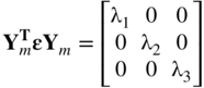
Because Ym is an orthogonal matrix, its columns define directions of three orthogonal axes called the principal axes or principal directions. The roots λ1, λ2, and λ3 are called the principal normal strains. Note that in the principal directions, the shear strains are identically equal to zero. Therefore, one can always select coordinate lines ![]() along which the shear strains vanish by using the coordinate transformation
along which the shear strains vanish by using the coordinate transformation ![]() . Equation 69 also shows that the strain tensor ϵ can be written as
. Equation 69 also shows that the strain tensor ϵ can be written as ![]() , which is the spectral decomposition of the strain tensor ϵ.
, which is the spectral decomposition of the strain tensor ϵ.
Strain Invariants
The following quantities associated with the strain tensor ϵ are called the principal strain invariants:
For the symmetric strain tensor ϵ, one can show that

The first strain invariant I1 = ϵ11 + ϵ22 + ϵ33 is called the dilatation or the volumetric strain.
Relationships between the principal values of different strain measures can be established. For example, the relationship between the principal values of the Green–Lagrange strain tensor and the principal values of the right Cauchy–Green deformation tensor can be developed using Equation 34, which when substituted into Equation 65 yields ({(Cr – I)/2} − λI)Y = 0. This equation shows that the principal values and principal directions of the deformation tensor Cr can be determined using the equation (Cr − (2λ + 1)I)Y = 0, which shows that ϵ and Cr have the same principal directions and also shows the difference between the principal values of the two deformation tensors. As will be shown in Chapter 4, there are material constitutive models, which are expressed in terms of the principal values and invariants of the deformation measures.
2.7 OBJECTIVITY
The concept of objectivity is important in solid mechanics and is associated with the study of the effect of the rigid-body motion. Quantities, such as strains, stresses, inertia, and distances between points, should satisfy certain requirements when the continuum experiences a rigid-body rotation, Stresses and deformation measures as well as their rate enter into the formulation of the material constitutive equations. It is important to make sure that the work of the resulting elastic forces and strain energy are not affected under pure rigid-body coordinate transformation. In particular, the stress and deformation measures used to define the elastic forces must be chosen such that the work of these forces and the strain energy remain constant when the continuum experiences a rigid-body rotation. In this case, the stresses and deformation measures are said to satisfy the objectivity requirement. In this book, we will not speak of objective variables, vectors, or tensors; instead we will speak of sets of variables that satisfy the objectivity requirement when used together in the formulation of the elastic forces. This is an approach slightly different from the one used in most continuum mechanics books to introduce the concept of objectivity.
In order to provide an introduction to the concept of objectivity, let A be the matrix that describes an arbitrary rigid-body rotation, and let ao and a be three-dimensional vectors on the continuous body before and after the rigid-body rotation, respectively. The relationship between the components of the vectors ao and a can be written as a = Aao. Note that in this case, despite the fact that ao and a have different components, they have the same length because A is an orthogonal matrix, and as a consequence, ![]() . Examples of vectors that satisfy this requirement are the vector dr that defines the line segment on the continuous body. For example, consider the two-step motion of a continuum. The first step is a general displacement defined by the reference coordinates x and current spatial coordinates ro. For this step, one can write dro = Jodx, and as a result
. Examples of vectors that satisfy this requirement are the vector dr that defines the line segment on the continuous body. For example, consider the two-step motion of a continuum. The first step is a general displacement defined by the reference coordinates x and current spatial coordinates ro. For this step, one can write dro = Jodx, and as a result ![]() , where in this equation, Jo is the matrix of position vector gradients. In the second step, the continuum undergoes a rigid-body rotation defined by the orthogonal transformation matrix A. If the spatial coordinates at the end of this step are defined by the vector r, one has dr = Adro = AJodx. Using the fact that A is an orthogonal transformation matrix, one has
, where in this equation, Jo is the matrix of position vector gradients. In the second step, the continuum undergoes a rigid-body rotation defined by the orthogonal transformation matrix A. If the spatial coordinates at the end of this step are defined by the vector r, one has dr = Adro = AJodx. Using the fact that A is an orthogonal transformation matrix, one has ![]() . That is, the length of the line segment does not change under an arbitrary rigid-body rotation.
. That is, the length of the line segment does not change under an arbitrary rigid-body rotation.
The analysis presented in this section shows that if a vector is defined on the continuum at any configuration, and the continuum experiences a pure rigid-body rotation from this configuration, the components of the vector defined in a selected global coordinate system will change as the result of this rigid-body rotation. Nonetheless, the length of the vector will not change. As will be discussed in this book, the elastic and dissipative forces due to the continuum displacements are expressed in terms of stress and deformation measures. Whereas some of these measures can change as the result of a rigid-body motion, it is required as previously stated that the work of the elastic forces and strain energy remain constant. It is, therefore, important to understand how different measures change as the result of the rigid-body rotation in order to be able to check the objectivity requirement.
In order to examine the change in the Green–Lagrange strain tensor as the result of the rigid-body rotation, we consider again a continuum at a certain configuration defined by the matrix of position vector gradients Jo. At this configuration, the Green–Lagrange strain tensor is defined as
Assume that the continuum experiences a rigid-body rotation from this configuration defined by the transformation matrix A. The new matrix of the position vector gradients can be written as J = AJo. It follows that the Green–Lagrange strain tensor for the final configuration is defined as
That is, Green–Lagrange strain tensor is not affected by the rigid-body rotation, an expected result based on the analysis previously presented in this chapter. It will be shown in the following chapter that the Green–Lagrange strain tensor is used with a stress tensor called the second Piola–Kirchhoff stress tensor to formulate the elastic forces. Because the Green–Lagrange strain tensor remains constant under an arbitrary rigid-body rotation, the second Piola–Kirchhoff stress tensor is also expected to remain constant in order to satisfy the objectivity requirement, and ensure that the work of the elastic forces and strain energy are not influenced by an arbitrary rigid-body coordinate transformation.
Next, we examine the effect of the rigid-body rotation on the velocity gradient tensor ![]() . Let again Jo and J be, respectively, the matrices of position vector gradients before and after the rigid-body rotation defined by the matrix A. Both Jo and J are defined by differentiation with respect to the same material coordinates x. As the result of the rigid-body rotation, J can be written in terms of Jo, as previously shown in this section, as J = AJo. Differentiating this equation with respect to time, one obtains
. Let again Jo and J be, respectively, the matrices of position vector gradients before and after the rigid-body rotation defined by the matrix A. Both Jo and J are defined by differentiation with respect to the same material coordinates x. As the result of the rigid-body rotation, J can be written in terms of Jo, as previously shown in this section, as J = AJo. Differentiating this equation with respect to time, one obtains
The velocity gradient tensor L is then defined as
which can be written using the fact that ![]() as
as
The second term on the right-hand side of this equation makes the velocity gradient tensor L unsuitable for use with a Lagrangian stress measure in the definition of the elastic forces, because when it is used with such Lagrangian stress measures, the objectivity requirement is not satisfied. Nonetheless, other stress measures, as discussed in Chapter 3, can be used with the velocity gradient tensor to formulate the energy balance equations.
The rate of deformation tensor, on the other hand, is often used with known stress measures to satisfy the objectivity requirement. In order to show the effect of the rigid-body rotation on the rate of deformation tensor D, one can write
Because ![]() , the preceding equation reduces to
, the preceding equation reduces to
This equation shows that the rate of deformation tensor is affected by the rigid-body rotation in a manner similar to some known stress measures. For this reason, D is used in several large deformation and plasticity constitutive models to account for the energy dissipation and at the same time to satisfy the objectivity requirement.
When studying the objectivity, it is important to distinguish between the change of the coordinate lines (parameters) and the change of the current configuration due to a rigid-body rotation. The change of the parameters does not lead to a change of the current configuration. Consider the change of the parameters from x1x2x3 to a new set of parameters along the axis of the coordinate system ![]() , as shown in Figure 5. Both coordinate systems are used with the same current configuration. Let A be the transformation matrix that defines the relationship between the two set of parameters. As previously discussed, the matrix of position vector gradients
, as shown in Figure 5. Both coordinate systems are used with the same current configuration. Let A be the transformation matrix that defines the relationship between the two set of parameters. As previously discussed, the matrix of position vector gradients ![]() associated with the coordinate system
associated with the coordinate system ![]() can be written in terms of the matrix of position vector gradients J associated with the coordinate system x1x2x3 using the equation
can be written in terms of the matrix of position vector gradients J associated with the coordinate system x1x2x3 using the equation ![]() . This gradient transformation does not change the vector r or the components of the line segment dr; it changes the definition of the reference coordinates (parameters) from x to
. This gradient transformation does not change the vector r or the components of the line segment dr; it changes the definition of the reference coordinates (parameters) from x to ![]() .
.
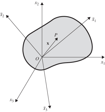
Figure 2.5 One current configuration and two reference coordinate systems (strain transformation)
On the other hand, a rigid-body rotation of the continuum from a given current configuration defines a new current configuration, as shown in Figure 6. If the rigid-body rotation is defined by the transformation matrix A, then the relationship between the new matrix of position vector gradients ![]() and the matrix of position vector gradients J associated with the previous current configuration is defined as
and the matrix of position vector gradients J associated with the previous current configuration is defined as ![]() . Note that this change of the current configuration changes the definition of the components of the vectors r and dr, whereas the coordinate lines ( parameters) remain the same.
. Note that this change of the current configuration changes the definition of the components of the vectors r and dr, whereas the coordinate lines ( parameters) remain the same.
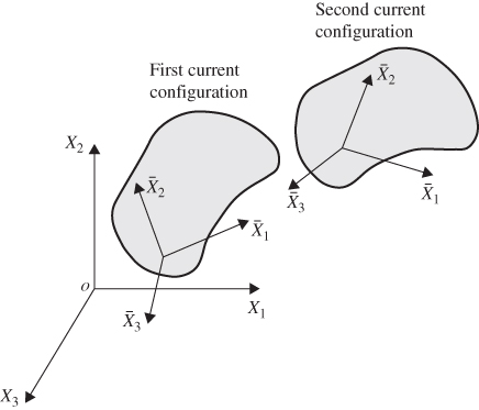
Figure 2.6 Two current configurations and one reference coordinate system (objectivity)
2.8 CHANGE OF VOLUME AND AREA
The relationships between the areas and volumes in the reference and current configurations are important in formulating the equations that define the effect of the inertia and elastic forces of the continuum. These relationships, which will be used in later chapters of this book, are obtained in this section. First, the relationship between the volumes is obtained and used to define the relationship between the areas.
Volume
The volume of an element can be obtained using the scalar triple product. Consider an element whose base is defined by the two vectors b and c, while another side is defined by the vector a. The volume of the element is defined as V = a · (b × c). The term (b × c) defines a vector whose magnitude is the area of the base and its direction is along a vector perpendicular to both b and c. In fact, the volume can be written using any cyclic permutation of the vectors a, b, and c, that is,
Now consider a volume element that has sides of length dx1, dx2, and dx3 in the reference configuration. The lengths of these line elements in the current configuration are given by dr1, dr2, and dr3, where

The length of the side of the volume element in the current configuration can then be defined in the direction of the parameters x1, x2, and x3 using the following three vectors:
The current volume of the element can then be written as
Because ![]() , and x1, x2, and x3 are defined along the orthogonal axes of a Cartesian coordinate system, that is, dx1dx2dx3 = dV is the volume of the element in the reference configuration, one has from the preceding equation, the following relationship between the volumes in the current and reference configurations:
, and x1, x2, and x3 are defined along the orthogonal axes of a Cartesian coordinate system, that is, dx1dx2dx3 = dV is the volume of the element in the reference configuration, one has from the preceding equation, the following relationship between the volumes in the current and reference configurations:
where J = |J|. In the case of small deformation, the determinant of J remains approximately equal to one, and the volume in the current configuration can be assumed to be equal to the volume in the reference configuration. Furthermore, if the determinant of J remains constant, the volume of the continuous body does not change. In this case, the displacement is called isochoric. The deformation of an incompressible material is isochoric because the volume does not change. Note also that if A is an orthogonal matrix, then |AJ| = |J| = J, which shows that the volume does not change under an arbitrary rigid-body motion.
Area
The relationship between the volumes in the reference and current configurations can be used to obtain the relationship between the areas. To this end, consider an area element defined in the reference and current configurations, respectively, by
where N and n are unit vectors normal to the areas in the reference and current configurations, respectively. Consider an arbitrary line element dx, which in the current configuration is defined by dr, where dr = Jdx. The corresponding volumes in the reference and current configurations are given by
Using Equation 83, it follows that
which upon using the fact that dr = Jdx, one obtains
Because dx is arbitrary, one has
In some references, this equation is called Nanson's formula (Ogden, 1984). Because N is a unit vector, it follows from Equation 88 that
or equivalently,

This equation defines the relationship between the area in the current configuration and the area in the reference configuration. Recall that the left Cauchy–Green deformation tensor Cl is defined as Cl = JJT. It follows that ![]() .
.
2.9 CONTINUITY EQUATION
If the mass is conserved, an element of mass dm can be written using the volumes and densities in the initial and current configurations as
In this equation, ρ0 and ρ are, respectively, the mass density in the initial and current configurations. Using the preceding equation and Equation 83, it is clear that
This equation, which is obtained using the principle of conservation of mass, is called the continuity equation. In the case of incompressible materials, the volume does not change and J = 1. In this case, the mass density remains constant; that is, ρ0 = ρ.
The continuity equation can be written in another form by considering the rates of the mass flow. If the mass is conserved, the rate at which an element mass increases must be equal to the rate at which the mass flows out of the element. Using the concept of a control volume, the element volume dv and the element area ds can be used to write the following conservation of mass equation:

In this equation, v is the velocity vector and n is the normal to the surface. Because n is used here to denote the outward normal, the negative sign is used. Furthermore, the partial derivative ∂ρ/∂t is used because the rate of change of the mass density ρ is assumed to be evaluated at a fixed point in the control volume. Using the divergence theorem, the surface integral can be written in terms of volume integral leading to
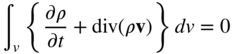
Because this equation must be satisfied everywhere in the continuum, one has
This is another form of the continuity equation, which can also be written as
or equivalently

In the case of incompressible materials, the mass density remains constant, that is, dρ/dt = 0. It then follows from the preceding equation that ![]() for incompressible materials. This implies that the trace of the rate of deformation tensor must be equal to zero if the incompressibility condition is imposed, that is, tr(D) = 0. This result will be used in Chapter 4 when the constitutive equations of the fluids are discussed.
for incompressible materials. This implies that the trace of the rate of deformation tensor must be equal to zero if the incompressibility condition is imposed, that is, tr(D) = 0. This result will be used in Chapter 4 when the constitutive equations of the fluids are discussed.
From the identities presented in the preceding chapter, one can write ![]() = Jtr(D) = Jtr(L) = Jdiv(v), where D and L are, respectively, the rate of deformation tensor and the velocity gradient tensor, and v is the velocity vector. Because ρ0 = ρJ, one has
= Jtr(D) = Jtr(L) = Jdiv(v), where D and L are, respectively, the rate of deformation tensor and the velocity gradient tensor, and v is the velocity vector. Because ρ0 = ρJ, one has ![]() . It follows that
. It follows that ![]() . This provides another simple derivation of the continuity equation (Ogden, 1984).
. This provides another simple derivation of the continuity equation (Ogden, 1984).
2.10 REYNOLDS' TRANSPORT THEOREM
In the preceding chapter, it was shown that the time rate of the change of the determinant of the Jacobian matrix J can be written as

In this equation, ![]() . The preceding equation can also be written as
. The preceding equation can also be written as
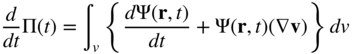
This equation can be used to obtain Reynolds' transport theorem, which defines the rate of change of a volume integral. Let Ψ (r, t) be any function defined in terms of the current configuration. The volume integral of this function is given as

Because the volume v is time varying, when evaluating the time rate of change of Π(t), one cannot take the differentiation through the integral sign. Using Equation 83, which relates the volumes in the current and reference configurations, Equation 100 can be written as
It follows that
This equation can be written as
Substituting Equation 98 into Equation 103, one obtains

This equation upon the use of Equation 83 can be written again in terms of the volume defined in the current configuration as
Because ![]() , the preceding equation can be rewritten as
, the preceding equation can be rewritten as
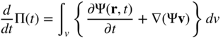
This equation, upon the use of the divergence theorem, can be written as

In this equation, s is the surface area in the current configuration, and n is the outward normal. The preceding equation, which is a statement of the Reynolds' transport theorem, shows that the rate of the change of the volume integral of the function Ψ(r, t) is the integral of the rate of change at the material points plus the net flow of Ψ(r, t) over the surface. In Reynolds' transport theorem, Ψ(r, t) can be a scalar, vector, or tensor function.
The principle of conservation of mass can be easily derived using the analysis presented in this section. To this end, the mass m of any volume can be written as
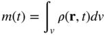
where ρ is the mass density in the current configuration. Letting Π = m and Ψ = ρ in Equation 106, one obtains in the case of conservation of mass

Because this equation is valid for an arbitrary volume, the integrand in this equation must be equal to zero everywhere. This leads to
which is the equation of continuity previously obtained in this chapter.
2.11 EXAMPLES OF DEFORMATION
In this section, several deformation examples are presented in order to shed light on some of the important concepts and definitions introduced in this chapter. Among these examples are the special case of planar deformation, extension and dilatational deformations, and shear deformation. The example of the two-dimensional beam used throughout this chapter will be used to demonstrate several deformation modes. The assumed displacement field used in this example is one of the displacement fields used in finite elements based on the absolute nodal coordinate formulation discussed in Chapter 5. This finite element formulation relaxes many of the assumptions used in classical beam and plate theories and, therefore, it can be conveniently used to demonstrate some of the general concepts discussed in this chapter.
Planar Displacement
In the case of planar displacement, the matrix of position vector gradients and its inverse take the following form:
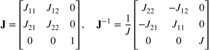
In this equation, J = J11J22 − J12J21 In this special case, ![]() does not change because the displacement is assumed to be planar. The Green–Lagrange strain tensor is defined as
does not change because the displacement is assumed to be planar. The Green–Lagrange strain tensor is defined as
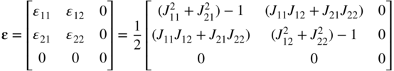
This equation shows that ϵ13, ϵ23, and ϵ33 are identically equal to zero. The velocity gradient tensor is

For such a planar motion, one can show that the rate of deformation and spin tensors are given, respectively, by

and
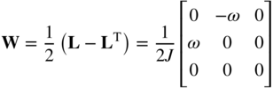
In this equation, ![]() . Note that the skew-symmetric spin tensor in the special case of planar rigid-body motion can be written as a function of the rate of one variable only. In the case of rigid-body motion, J = 1, J11 = J22 = cos θ, and J21 = −J12 = sin θ, where θ is the angle of the rigid-body rotation. It follows in this case that the rate of deformation tensor D is identically zero, and the spin tensor W is
. Note that the skew-symmetric spin tensor in the special case of planar rigid-body motion can be written as a function of the rate of one variable only. In the case of rigid-body motion, J = 1, J11 = J22 = cos θ, and J21 = −J12 = sin θ, where θ is the angle of the rigid-body rotation. It follows in this case that the rate of deformation tensor D is identically zero, and the spin tensor W is

Extension and Stretch
If the gradient vectors change their lengths but remain orthogonal, one obtains pure extension or stretch; the most general case of which is the dilatational deformation. In this case, the matrix of position vector gradients can be written as J = RU, where R is an orthogonal matrix and U is a diagonal stretch matrix given as
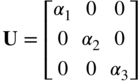
where αi is the stretch in the ith direction. That is, ![]() . The Green–Lagrange strain tensor can be written as
. The Green–Lagrange strain tensor can be written as

This equation shows that all the shear strain components are identically equal to zero and the motion is a dilatational deformation. Because U and ![]() are diagonal, one can show that the rate of deformation tensor can be written as
are diagonal, one can show that the rate of deformation tensor can be written as
Because both U and ![]() are diagonal, the rate of deformation tensor D is also a diagonal tensor with diagonal elements
are diagonal, the rate of deformation tensor D is also a diagonal tensor with diagonal elements ![]() .
.
For this mode of purely extension deformations, the diagonal elements of the Green–Lagrange strains of Equation 118 are the principal values, and the coordinate axes define the principal directions because the shear stresses are identically equal to zero. Because the trace and determinant are among the invariants of a second-order tensor, one can show that an orthogonal coordinate transformation does not change the values of these diagonal elements. Extensions in only one or two directions can be obtained as special cases of the model presented in this section.
Several classical formulations used in the small- and large-deformation analysis of beams and plates do not capture some stretch modes. For example, classical beam theories assume that the beam cross section remains rigid. That is, when the beam experiences bending, for example, the dimensions of the beam cross section do not change. Although such an assumption can be acceptable for small-deformation problems, the theories based on this assumption cannot be used to correctly predict the behavior of beams when they are subjected to large and inelastic deformations. Such simplified theories cannot also be used to fully capture Poisson effect, which results in change of the cross-sectional dimensions when the beam is subjected to elongation or bending. The material constitutive equations couple the normal strains, leading to normal stresses (positive or negative) in the plane of the cross section. With some of the existing nonlinear formulations, such a Poisson effect cannot be captured. This represents a serious limitation when considering applications related to mechanical, aerospace, biomedical, and biological systems in which the deformations of the cross sections can have a significant effect. Modeling the structural stiffness of ligaments, muscles, and DNA as well as many other engineering and biomedical applications are among the examples that require a more general approach that allows implementing more general constitutive models. In Chapter 5, a nonlinear formulation that captures the Poisson effect and other coupled modes of deformation is discussed in more detail. The displacement field used in the following example is one of the displacement fields used for the finite element absolute nodal coordinate formulation discussed in Chapter 5.
Shear Deformation
If the lengths of all the gradient vectors remain constant, the normal strains in the defined configuration will not change as is clear from the definition of the Green–Lagrange strain tensor. If the motion is the result of only the change of the relative orientation between the gradient vectors, one obtains the case of shear deformations. In this case, the Green–Lagrange strain tensor can be written as

That is, the normal strains are zeros; however, the shear strains are functions of the angles between the gradient vectors. It is left to the reader to examine the effect of the coordinate transformation on the form of the Green–Lagrange strain tensor when the lengths of the gradient vectors remain constant.
The preceding example sheds light on the strain transformation and the change of the strain definitions in different planes and coordinate systems. Note that in the special planar case, the general form of the symmetric strain tensor can be written as

The definition of this strain tensor in another coordinate system whose orientation is defined by the transformation matrix A is given as previously mentioned by the equation ![]() . Let the matrix A be defined using the general planar transformation
. Let the matrix A be defined using the general planar transformation

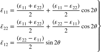
Then the components of the symmetric strain tensor are defined as

This equation can also be written in the following form:

This equation is the basis for a graphical representation known as Mohr's circle (Ugural and Fenster, 1979). The orientation of the coordinate system in which the maximum normal strains are defined can be obtained by differentiating one of the first two equations in Equation 124 with respect to θ. This defines the angle θ that can be substituted back into the first two equations to determine the principal strains. This procedure for determining the principal normal strains and principal directions is equivalent to the use of the eigenvalue analysis previously discussed in this chapter.
If the coordinate system is selected such that the normal strains are zero, as in the case of the preceding example, one has ϵ11 = ϵ22 = 0. In this case, Equation 124 leads to
The orientation of a coordinate system, which gives the maximum normal strains, can be determined using the preceding equation as
which have solution θ = π/4, an angle that defines the coordinate system in which the normal strains are maximum or minimum. Equation 125 shows that in this new coordinate system, ![]() is identically equal to zero. This result was obtained in the preceding example using the eigenvalue analysis.
is identically equal to zero. This result was obtained in the preceding example using the eigenvalue analysis.
Alternatively, if one starts with a coordinate system in which the shear strains are equal to zero, Equation 124 yields
The orientation of the coordinate system in which the shear strain is maximum can be determined from the following equation:
This equation defines again θ = π/4. Substituting this value of θ in the first two equations of Equation 127, one does not obtain zero normal strains.
2.12 GEOMETRY CONCEPTS
In many applications, the position vector gradients in the undeformed reference configuration are not orthogonal unit vectors because of the continuum initial geometry. Examples of these applications, which include tires, belt drives, and tank cars, are shown in Figure 8. In these cases, the strains evaluated using the matrix of position vector gradients in the initial configuration must be identically equal to zero. In order to explain how the strains are formulated in these cases of initial curved geometry, the three different configurations shown in Figure 9 are considered in this section. Complex geometries can always be obtained by changing the shape of simple objects; the first configuration in Figure 9 depicts the simple geometry, which can represent straight metal sheets. In this simple geometry configuration, the location of the material points is defined using the position vector ![]() . The second configuration is the reference configuration, which defines the initial undeformed geometry. In this undeformed reference configuration, the position of the material points is defined by the vector
. The second configuration is the reference configuration, which defines the initial undeformed geometry. In this undeformed reference configuration, the position of the material points is defined by the vector ![]() . One can write
. One can write ![]() , where
, where ![]() . The third configuration shown in Figure 9 defines the current deformed configuration. In this configuration, the position of the material points is defined by the vector
. The third configuration shown in Figure 9 defines the current deformed configuration. In this configuration, the position of the material points is defined by the vector ![]() . One can then write
. One can then write ![]() , with
, with ![]() . It follows that
. It follows that ![]() , where
, where ![]() .
.
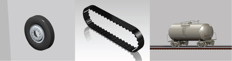
Figure 2.8 Initial geometry
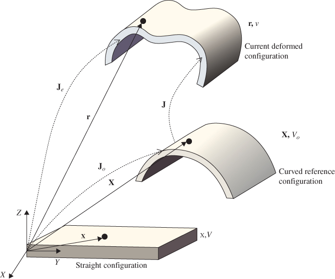
Figure 2.9 Geometry description
The volume of the curved structure ![]() is related to the volume of the straight structure
is related to the volume of the straight structure ![]() (Figure 9) using the relationship
(Figure 9) using the relationship ![]() , where
, where ![]() is the determinant of the matrix of position vector gradients
is the determinant of the matrix of position vector gradients ![]() . Therefore, integration with respect to the domain
. Therefore, integration with respect to the domain ![]() can be converted to integration with respect to the straight domain
can be converted to integration with respect to the straight domain ![]() by using the transformation
by using the transformation ![]() . This allows for using the original dimensions of the simpler geometry to carry out the integrations associated with the initially curved configuration. Note that the matrix
. This allows for using the original dimensions of the simpler geometry to carry out the integrations associated with the initially curved configuration. Note that the matrix ![]() is constant.
is constant.
The matrix of position vector gradients ![]() is the matrix, used to determine the Lagrangian strain tensor
is the matrix, used to determine the Lagrangian strain tensor ![]() as
as ![]() . This matrix can be defined using the ANCF description introduced in Chapter 5 as
. This matrix can be defined using the ANCF description introduced in Chapter 5 as
where, as previously defined, ![]() . Therefore, the Lagrangian strain tensor can be written as
. Therefore, the Lagrangian strain tensor can be written as
Recall that the relationship between the volume in the current deformed configuration ![]() and the volume in the curved reference configuration
and the volume in the curved reference configuration ![]() can be written as
can be written as ![]() , where
, where ![]() is the determinant of the matrix of position gradients
is the determinant of the matrix of position gradients ![]() . It follows that
. It follows that ![]() . Using the relationship
. Using the relationship ![]() , one has
, one has ![]() .
.
The procedure described in this section to model the initial curvature, which is the same as the one used in the literature for modeling the initially curved configuration of belt drives and rubber chains (Dufva et al., 2007; and Maqueda et al., 2010), will lead to zero strains for an arbitrary initially curved geometry. Using the ANCF finite elements discussed later in this book, the constant matrix of position vector gradients ![]() can be determined in a straightforward manner.
can be determined in a straightforward manner.
PROBLEMS
-
1 The assumed displacement field of a two-dimensional beam is given by r = Se, where S is a 2 × 8 shape function matrix defined as

In this equation, I is a 2 × 2 identity matrix and

where ξ = x1/l and l is the length of the beam. The vector of time-dependent coordinates e is defined as

Show that this displacement field can describe an arbitrary planar rigid-body motion.
-
2 Show that the Green–Lagrange strain tensor does not lead to zero strains under an arbitrary rigid-body motion if nonlinear terms of the displacement gradients that appear in the definition of this strain tensor are neglected.
-
3 Let ϵ = (ld − lo)/lo (see Equation 21). For the problem in Example 3, determine ϵ using Equation 24 at x1 = 0.5 l and x1 = l for the following two cases of nodal coordinates assuming that t = [1 0]T:

-
4 Instead of the definition of ϵ given by Equation 21, define ϵ = (ld − lo)/ld. Using this definition, determine an expression of ϵ (similar to Equation 24) in terms of the Eulerian strain tensor.
-
5 Using the definition of ϵ in the preceding problem, determine the Eulerian strain tensor and ϵ at x1 = 0.5 l and x1 = l for the two cases of Problem 3.
-
6 For the problem in Example 3, discuss the differences between the Green–Lagrange and Eulerian strain tensors in the case of arbitrary deflection δ.
-
7 For the problem in Example 3, determine the right and left Cauchy–Green deformation tensors for the two different sets of nodal coordinates.
-
8 For the problem in Example 4, show whether or not the right and left Cauchy–Green strain tensors depend on the rotation angle θ.
-
9 For the problem in Example 3, determine the polar decomposition of the matrix of position vector gradients for (δ/l) = 0.1 at x1 = 0.5 l and x1 = l for the two different sets of nodal coordinates. Determine both the right and left symmetric stretch matrices.
-
10 In the problem of Example 3, determine the rate of deformation tensor assuming that
 is known.
 -
11 Repeat Example 6, assuming that the elongation δ is not constant.
-
12 The Green–Lagrange strain tensor at a given point on the continuous body is defined as

Determine the principal values, principal directions, and the strain invariants.
-
13 Discuss the difference between the change of the reference coordinate system and the change of the current configuration.
-
14 Show that
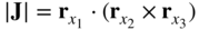 , where |J| is the determinant of the matrix of position vector gradients.