Chapter 8
The Basics of Spreadsheets: Numbers, Labels, and Formulas
IN THIS CHAPTER
Typing and formatting data
Moving around a spreadsheet
Searching a spreadsheet
Editing a spreadsheet
Printing
Everyone needs to perform simple math. Businesses need to keep track of sales and profits, and individuals need to keep track of budgets. In the old days, people not only had to write down numbers on paper, but they also had to do all their calculations by hand (or with the aid of a calculator).
That’s why people use Excel. Instead of writing numbers on paper, they can type numbers on the computer. Instead of adding or subtracting columns or rows of numbers by hand, they can let Excel do it faster. By using Excel, you can focus on typing in the correct numbers and let Excel worry about calculating accurate results quickly.
 Besides calculating numbers, spreadsheets can also store lists of data organized in rows and columns.
Understanding Spreadsheets
Excel organizes numbers in rows and columns. An entire page of rows and columns is called a spreadsheet or a worksheet. (A collection of one or more worksheets is stored in a file called a workbook.) Each row is identified by a number such as 1 or 249; and each column is identified by letters, such as A, G, or BF. The intersection of each row and column defines rectangular spaces called cells, each of which contains one of three items:
- Numbers
- Text (labels)
- Formulas
Numbers provide the data, and formulas calculate that data to produce a useful result, such as adding sales results for the week. Of course, just displaying numbers on the screen may be confusing if you don’t know what those numbers mean, so labels simply identify what numbers represent. Figure 8-1 shows the parts of a typical spreadsheet.

FIGURE 8-1: The parts of a typical spreadsheet.
Formulas usually appear as numbers, so at first glance, it may be difficult to tell the difference between ordinary numbers and numbers that represent a calculation by a formula.
The strength of spreadsheets comes by playing “What-if?” games with your data, such as “What if I gave myself a $20-per-hour raise and cut everyone else’s salary by 25%? How much money would that save the company every month?” Because spreadsheets can rapidly calculate new results, you can experiment with different numbers to see how they create different answers.
Storing Stuff in a Spreadsheet
Every cell can contain a number, a label, or a formula. To type anything into a spreadsheet, you must first select or click in the cell (or cells) and then type a number or text.
Typing data into a single cell
To type data in a single cell, follow these steps:
- Choose one of the following to select a single cell:
- Click a cell.
- Press the up/down/right/left arrow keys to highlight a cell.
-
Type a number (such as 34.29 or 198), a label (such as Tax Returns), or a formula.
You can see how to create formulas in Chapter 9.
Typing data in multiple cells
After you type data in a cell, you can press one of the following four keystrokes to select a different cell:
- Enter: Selects a cell below
- Tab: Selects the cell to the right in the same row
- Shift+Enter: Selects the cell above in the same column
- Shift+Tab: Selects the cell to the left in the same row
If you type data in cell A1 and press Enter, Excel selects the next cell below, which is A2. If you type data in A2 and press Tab, Excel selects the cell to the right, which is B2.
However, what if you want to type data in a cell such as A1 and then have Excel select the next cell to the right (B1)? Or what if you want to type data in cells A1 and A2 but then jump back to type additional data in cells B1 and B2?
To make this easy, Excel lets you select a range of cells, which essentially tells Excel, “See all the cells I just highlighted? I only want to type data in those cells.” After you select multiple cells, you can type data and press Enter. Excel selects the next cell down in that same column. When Excel reaches the last cell in the column, it selects the top cell of the column to the right.
To select multiple cells for typing data in, follow these steps:
-
Highlight multiple cells by choosing one of the following:
- Move the mouse pointer over a cell, hold down the left mouse button, and drag (move) the mouse to highlight multiple cells. Release the left mouse button when you’ve selected enough cells.
- Hold down the Shift key and press the up/down/right/left arrow keys to highlight multiple cells. Release the Shift key when you’ve selected enough cells.
Excel selects the cell that appears in the upper-left corner of your selected cells.
- Type a number, label, or formula.
-
Press Enter.
Excel selects the cell directly below the preceding cell. If the preceding cell appeared at the bottom of the selected column, Excel highlights the top cell in the column that appears to the right.
 You can also move backward by pressing Shift+Enter instead.
 - Repeat Steps 2 and 3 until you fill your selected cells with data.
- Click outside the selected cells or press an arrow key to tell Excel not to select the cells anymore.
Typing in sequences with AutoFill
If you need to type the names of successive months or days in a row or column (such as January, February, March, and so on), Excel offers a shortcut to save you from typing all the day or month names yourself. With this shortcut, you just type one month or day and then drag the mouse to highlight all the adjacent cells. Then Excel types the rest of the month or day names in those cells automatically.
To use this shortcut, follow these steps:
-
Click a cell and type a month (such as January or just Jan) or a day (such as Monday or just Mon).
The Fill Handle, a box, appears in the bottom-right corner of the cell.
You can also type in a sequence of numbers in Step 1. So if you typed the numbers 2, 4, and 6 in adjacent cells, highlighted all these adjacent cells, and grabbed the Fill Handle, Excel is smart enough to detect the pattern and display the numbers 8, 10, and 12 in the next three adjacent cells. - Move the mouse pointer over the Fill Handle until the mouse pointer turns into a black crosshair icon.
-
Hold down the left mouse button and drag (move) the mouse down a column or across the row.
As you drag the mouse, Excel displays the remaining month or day names that it will add to the cells, as shown in Figure 8-2.

FIGURE 8-2: When you drag the Fill Handle, Excel automatically enters the names of the month or days.
Formatting Numbers and Labels
When you first create a spreadsheet, numbers and labels appear as plain text. Plain labels may look boring, but plain numbers (such as 8495 or 0.39) can be difficult to read and understand if the numbers are supposed to represent currency amounts ($8,495) or percentages (39%).
To make labels visually interesting and numbers appear more descriptive of what they actually represent, you need to format your data after you type it into a spreadsheet.
You can format a cell or range of cells after you’ve already typed in data or before you type in any data. If you format cells before typing any data, any data you type in that cell will appear in your chosen format.
Formatting numbers
To format the appearance of numbers, follow these steps:
-
Select one or more cells by using the mouse or keyboard.
To select multiple cells, drag the mouse or hold the Shift key while pressing the arrow keys.
- Click the Home tab.
-
Click the Number Format list box in the Number group.
A pull-down menu appears, as shown in Figure 8-3.
The Number group also displays three icons that let you format numbers as Currency, Percentage, or with Commas in one click, as shown in Figure 8-4. If you click the downward-pointing arrow to the right of the Accounting Number Format icon, you can choose different currency symbols to use, such as $, £, or €. -
Click a number format style, such as Percentage or Scientific.
Excel displays your numbers in your chosen format.

FIGURE 8-3: The Number Format list box lists the different ways you can format the appearance of numbers.

FIGURE 8-4: The different ways you can format money.
Displaying negative numbers
Because many people use spreadsheets for business, they often want negative numbers to appear highlighted so they can see them easier. Excel can display negative numbers in parentheses (–23) or in red so you can’t miss them.
To define how negative numbers appear in your spreadsheet, follow these steps:
- Select the cell or range of cells that you want to modify.
- Click the Home tab.
-
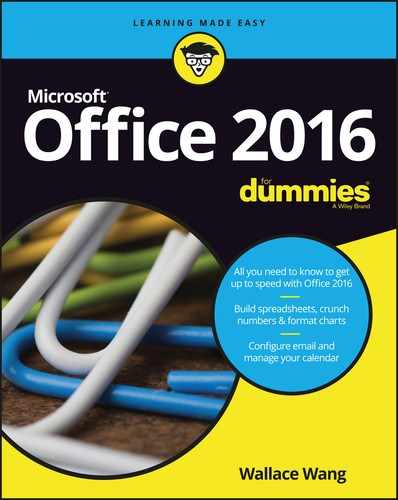
Click the Format icon in the Cells group.
A menu appears, as shown in Figure 8-5.
-
Choose Format Cells.
The Format Cells dialog box appears, as shown in Figure 8-6.
-
Choose Currency or Number from the Category list.
You can choose how to format negative numbers only if you format your numbers by using the Currency or Number category. -
Click a negative number format and then click OK.
If any of your numbers become negative in the cell or cells you select in Step 1, Excel automatically displays those negative numbers in the negative number format you choose.
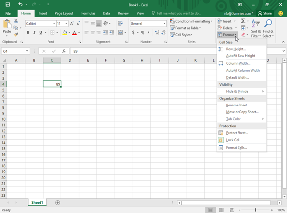
FIGURE 8-5: The Format icon lets you format the appearance of rows, columns, or individual cells.

FIGURE 8-6: The Format Cells dialog box lets you customize the appearance of your numbers.
Formatting decimal numbers
If you format cells to display numbers with decimal places, such as 23.09 or 23.09185, you can modify how many decimal places appear. To define the number of decimal places, follow these steps:
- Select the cell or cells that contain the numbers you want to format.
- Click the Home tab.
-
Click in the Number Format list box (refer to Figure 8-3) and choose a format that displays decimal places, such as Number or Percentage.
Excel formats the numbers in your chosen cells.
You can click the Increase Decimal (increases the number of decimal places displayed) or Decrease Decimal icon (decreases the number of decimal places displayed) in the Number group on the Home tab, as shown in Figure 8-7.

FIGURE 8-7: A click quickly changes the number of decimal places displayed.
Formatting cells
To make your data look prettier, Excel can format the appearance of cells to change the font, background color, text color, or font size used to display data in a cell.
Excel provides two ways to format cells: You can use Excel’s built-in formatting styles, or you can apply different types of formatting individually. Some of the individual formatting styles you can choose include
- Font and font size
- Text styles (underlining, italic, and bold)
- Text and background color
- Borders
- Alignment
- Text wrapping and orientation
Formatting cells with built-in styles
Excel provides a variety of predesigned formatting styles that you can apply to one or more cells. To format cells with a built-in style, follow these steps:
- Select the cell or cells that you want to format with a built-in style.
- Click the Home tab.
-
Click the Cell Styles icon in the Styles group.
A pull-down menu appears listing all the different styles you can choose, as shown in Figure 8-8.
-
Move the mouse pointer over a style.
Excel displays a Live Preview of how your selected cells will look with that particular style.
-
Click the style you want.
Excel applies your chosen style to the selected cells.

FIGURE 8-8: The Cell Styles menu offers different ways to format your cells quickly.
Formatting fonts and text styles
Different fonts can emphasize parts of your spreadsheet, such as using one font to label columns and rows and another font or font size to display the actual data. Text styles (bold, underline, and italic) can also emphasize data that appears in the same font or font size.
To change the font, font size, and text style of one or more cells, follow these steps:
- Select the cell or cells that you want to change the font and font size.
- Click the Home tab.
-
Click the Font list box.
A pull-down menu of different fonts appears.
- Click the font you want to use.
- Choose one of the following methods to change the font size:
- Click the Font Size list box and then choose a font size, such as 12 or 16.
- Click the Font Size list box and type a value such as 7 or 15.
- Click the Increase Font Size or Decrease Font Size icon until your data appears in the size you want.
- Click one or more text style icons (Bold, Italic, Underline).
Formatting with color
Each cell displays data in a Font color and a Fill color. The Font color defines the color of the numbers and letters that appear inside a cell. (The default Font color is black.) The Fill color defines the color that fills the background of the cell. (The default Fill color is white.)
To change the Font and Fill colors of cells, follow these steps:
- Select the cell or cells that you want to color.
- Click the Home tab.
-
Click the downward-pointing arrow that appears to the right of the Font Color icon (the icon looks like a capital A).
A color palette appears, as shown in Figure 8-9.
-
Click the color you want to use for your text.
The color you select appears directly on the Font Color icon. The next time you want to apply this same color to a cell, you can click the Font Color icon directly instead of the downward-pointing arrow to the right of the Font Color icon. -
Click the downward-pointing arrow that appears to the right of the Fill Color icon (the icon looks like a pouring bucket).
A color palette appears.
-
Click a color to use to fill the background of your cell.
The color you select appears directly on the Fill Color icon. The next time you want to apply this same color to a cell, you can click the Fill Color icon directly instead of the downward-pointing arrow to the right of the Fill Color icon.
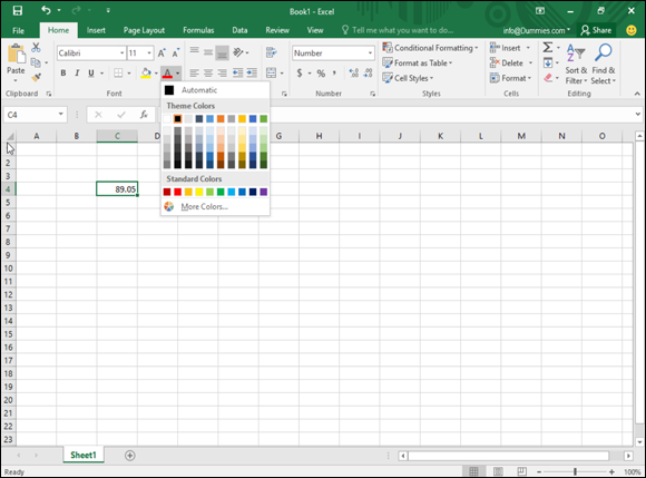
FIGURE 8-9: You can display data and the background of each cell in a different color.
Adding borders
For another way to highlight one or more cells, you can add borders. Borders can surround the entire cell or just the top, bottom, left, or right side of a cell. To add borders to a cell, follow these steps:
- Select one or more cells.
- Click the Home tab.
-
Click the downward-pointing arrow to the right of the Border icon in the Font group.
A pull-down menu appears, as shown in Figure 8-10.
-
Click a border style.
Excel displays your chosen borders around the cells you selected in Step 1.

FIGURE 8-10: The Border menu lists different ways to place borders around cells.
Navigating a Spreadsheet
If you have a large spreadsheet, chances are good that some information may be hidden by the limitations of your computer screen. To help you view and select cells in different parts of your spreadsheet, Excel offers various ways to navigate a spreadsheet by using the mouse and keyboard.
Using the mouse to move around in a spreadsheet
To navigate a spreadsheet with the mouse, you can click the onscreen scroll bars or use the scroll wheel on your mouse (if it has one). To use the scroll bars, you have three choices:
-
Click the up/down or right/left arrows on the horizontal or vertical scroll bars.
This moves the spreadsheet one row (up or down) or column (right or left) at a time.
- Drag the scroll box of a scroll bar.
-
Click the scroll area (any area to the left/right or above/below the scroll box on the scroll bar).
This moves the spreadsheet one screen left/right or up/down.
If your mouse has a scroll wheel, you can use this wheel to move through a spreadsheet by two methods:
- Roll the mouse’s scroll wheel forward or back to scroll your spreadsheet up or down.
- Press the scroll wheel to display a four-way pointing arrow, and then move the mouse up, down, right, or left. (When you’re done, click the scroll wheel again.)
Using the keyboard to move around a spreadsheet
Using the mouse can be a faster way to jump from one place in a spreadsheet to another, but sometimes trying to line up the mouse just right can be frustrating. For that reason, you can also use the keyboard to move around a spreadsheet. Some of the common ways to move around a spreadsheet are shown in Table 8-1.
TABLE 8-1: Using the Keyboard to Navigate a Spreadsheet
|
Pressing This |
Does This |
|
Up arrow (↑) |
Moves up one row |
|
Down arrow (↓) |
Moves down one row |
|
Left arrow (←) |
Moves left one column |
|
Right arrow (→) |
Moves right one column |
|
Ctrl+↑ |
Jumps up to the top of a column that contains data |
|
Ctrl+↓ |
Jumps down to the bottom of a column that contains data |
|
Ctrl+← |
Jumps to the left of a row that contains data |
|
Ctrl+→ |
Jumps to the right of a row that contains data |
|
Page Up |
Moves up one screen |
|
Page Down |
Moves down one screen |
|
Ctrl+Page Up |
Displays the previous worksheet |
|
Ctrl+Page Down |
Displays the next worksheet |
|
Home |
Moves to the A column of the current row |
|
Ctrl+Home |
Moves to the A1 cell |
|
Ctrl+End |
Moves to the bottom-right cell of your spreadsheet |
If you know the specific cell you want to move to, you can jump to that cell by using the Go To command. To use the Go To command, follow these steps:
- Click the Home tab.
-
Click the Find & Select icon in the Editing group.
A pull-down menu appears.
-
Click Go To.
The Go To dialog box appears, as shown in Figure 8-11.
You can also choose the Go To command by pressing Ctrl+G. -
Click in the Reference text box and type the cell you want to move to, such as C13 or F4.
If you’ve used the Go To command before, Excel lists the last cell references you typed. Now you can just click one of those cell references to jump to that cell. -
Click OK.
Excel highlights the cell you typed in Step 4.

FIGURE 8-11: The Go To dialog box lets you jump to a specific cell.
Naming cells
One problem with the Go To command is that most people won’t know which cell contains the data they want to find. For example, if you want to view the cell that contains the total amount of money you owe for your income taxes, you probably don’t want to memorize that this cell is G68 or P92.
To help you identify certain cells, Excel lets you give them descriptive names. To name a cell or range of cells, follow these steps:
- Select the cell or cells that you want to name.
- Click in the Name box, which appears directly above the A column heading, as shown in Figure 8-12.
- Type a descriptive name without any spaces and then press Enter.

FIGURE 8-12: You can type a descriptive name for your cells in the Name box.
After you name a cell, you can jump to it quickly by following these steps:
-
Click the downward-pointing arrow to the right of the Name box.
A list of named cells appears.
-
Click the named cell you want to view.
Excel displays your chosen cell.
Eventually, you may want to edit or delete a name for your cells. To delete or edit a name, follow these steps:
- Click the Formulas tab.
-
Click the Name Manager icon.
The Name Manager dialog box appears, as shown in Figure 8-13.
- Edit or delete the named cell as follows:
- To edit the name, click the cell name you want to edit and then click the Edit button. An Edit Name dialog box appears, where you can change the name or the cell reference.
- To delete the name, click the cell name you want to delete and then click the Delete button.
- Click Close.

FIGURE 8-13: The Name Manager dialog box lets you rename or delete previously named cells.
Searching a Spreadsheet
Rather than search for a specific cell, you may want to search for a particular label or number in a spreadsheet. Excel lets you search for the following:
- Specific text or numbers
- All cells that contain formulas
- All cells that contain conditional formatting
Searching for text
You can search for a specific label or number anywhere in your spreadsheet. To search for text or numbers, follow these steps:
- Click the Home tab.
-
Click the Find & Select icon in the Editing group.
A pull-down menu appears.
-
Click Find.
The Find and Replace dialog box appears, as shown in Figure 8-14.
If you click the Replace tab, you can define the text or number to find and new text or numbers to replace it. -
Click in the Find What text box and type the text or number you want to find.
If you click the Options button, the Find and Replace dialog box expands to provide additional options for searching, such as searching in the displayed sheet or the entire workbook. - Click one of the following:
- Find Next: Finds and selects the first cell, starting from the currently selected cell that contains the text you typed in Step 4.
- Find All: Finds and lists all cells that contain the text you typed in Step 4, as shown in Figure 8-15.
- Click Close to make the Find and Replace dialog box go away.

FIGURE 8-14: The Find and Replace dialog box lets you search your worksheet.

FIGURE 8-15: The Find All button names all the cells that contain the text or number you want to find.
Searching for formulas
Formulas appear just like numbers; to help you find which cells contain formulas, Excel gives you two choices:
- Display formulas in your cells (instead of numbers).
- Highlight the cells that contain formulas.
To display (or hide) formulas in a spreadsheet, you have two options:
- Press Ctrl+` (an accent grave character, which appears on the same key as the ~ sign, often to the left of the number 1 key near the top of a keyboard).
- Click the Formulas tab, then click Show Formulas.
Figure 8-16 shows what a spreadsheet looks like when formulas appear inside of cells.

FIGURE 8-16: By displaying formulas in cells, you can identify which cells display calculations.
To highlight all cells that contain formulas, follow these steps:
- Click the Home tab.
-
Click the Find & Select icon in the Editing group.
A pull-down menu appears.
-
Click Formulas.
Excel highlights all the cells that contain formulas.
Editing a Spreadsheet
The two ways to edit a spreadsheet are
- Edit the data itself, such as the labels, numbers, and formulas that make up a spreadsheet.
- Edit the physical layout of the spreadsheet, such as adding or deleting rows and columns, or widening or shrinking the width or height of rows and columns.
Editing data in a cell
To edit data in a single cell, follow these steps:
-
Double-click the cell that contains the data you want to edit.
Excel displays a cursor in your selected cell.
- Edit your data by using the Backspace or Delete key, or by typing new data.
If you click a cell, Excel displays the contents of that cell in the Formula bar. You can click and edit data directly in the Formula bar, which can be more convenient for editing large amounts of data such as a formula.
Changing the size of rows and columns with the mouse
Using the mouse can be a quick way to modify the sizes of rows and columns. To change the height of a row or the width of a column, follow these steps:
-
Move the mouse pointer over the bottom line of a row heading, such as the 2 or 18 heading. (Or move the mouse pointer over the right line of the column heading, as for column A or D.)
The mouse pointer turns into a two-way pointing arrow.
-
Hold down the left mouse button and drag (move) the mouse.
Excel resizes your row or column.
- Release the left mouse button when you’re happy with the size of your row or column.
Typing the size of rows and columns
If you need to resize a row or column to a precise value, it’s easier to type a specific value into the Row Height or Column Width dialog box instead. To type a value into a Row Height or Column Width dialog box, follow these steps:
- Click the Home tab.
-
Click the row or column heading that you want to resize.
Excel highlights your entire row or column.
-
Click the Format icon that appears in the Cells group.
A pull-down menu appears, as shown in Figure 8-17.
-
Click Row Height (if you selected a row) or Column Width (if you selected a column).
The Row Height or Column Width dialog box appears.
-
Type a value and then click OK.
Excel resizes your row or column.

FIGURE 8-17: The Format icon lets you adjust the size of rows and columns.
Excel measures column width in characters. (A cell defined as 1 character width can display a single letter or number.) Excel measures row height by points where 1 point equals ![]() inch.
inch.
Adding and deleting rows and columns
After you type labels, numbers, and formulas, you may suddenly realize that you need to add or delete extra rows or columns. To add a row or column, follow these steps:
- Click the Home tab.
-
Click the row or column heading where you want to add another row or column.
Excel highlights the entire row or column.
-
Click the downward-pointing arrow of the Insert icon in the Cells group.
A menu appears.
-
Choose Insert Sheet Rows or Insert Sheet Columns.
Excel inserts a new row above the selected row or inserts a column to the left of the selected column.
For a fast way to insert a row or column, right-click on a row or column heading; when a pop-up menu appears, choose Insert. This inserts a column to the left of the column you right-clicked, or inserts a row above the row you right-clicked.
To delete a row or column, follow these steps:
- Click the Home tab.
- Click the row or column heading that you want to delete.
-
Click the downward-pointing arrow of the Delete icon in the Cells group.
A pull-down menu appears.
- Choose Delete Sheet Rows or Delete Sheet Columns.
 Deleting a row or column deletes any data stored in that row or column.
Adding sheets
For greater flexibility, Excel lets you create individual spreadsheets that you can save in a single workbook (file). When you load Excel, it automatically provides you with a sheet, but you can add more if you need them.
To add a new sheet, choose one of the following:
- Click the New sheet icon (it looks like a plus sign inside a circle) that appears to the right of your existing tabs (or press Shift+F11), as shown in Figure 8-18.
- Click the Home tab, click the Insert icon in the Cells group, and when a menu appears, choose Insert Sheet.

FIGURE 8-18: Excel displays the names of individual sheets as tabs.
Renaming sheets
By default, Excel gives each sheet a generic name such as Sheet1. To give your sheets a more descriptive name, follow these steps:
- Choose one of the following:
-
Double-click the sheet tab that you want to rename.
Excel highlights the entire sheet name.
- Click the sheet tab you want to rename, click the Home tab, click the Format icon in the Cells group, and choose Rename Sheet.
- Right-click the sheet tab you want to rename; when a pop-up menu appears, choose Rename.
-
-
Type a new name for your sheet and press Enter when you’re done.
Your new name appears on the sheet tab.
Rearranging sheets
You can rearrange the order that your sheets appear in your workbook. To rearrange a sheet, follow these steps:
- Move the mouse pointer over the sheet tab that you want to move.
-
Hold down the left mouse button and drag (move) the mouse.
The downward-pointing black arrow points where Excel will place your sheet.
- Release the left mouse button to place your sheet in a new order.
Deleting a sheet
Using multiple sheets may be handy, but you may want to delete a sheet if you don’t need it.
If you delete a sheet, you also delete all the data stored on that sheet.
To delete a sheet, follow these steps:
- Click the sheet that you want to delete.
-
Choose one of the following:
- Right-click the tab of the sheet you want to delete. When a pop-up menu appears, click Delete.
- Click the Home tab, click the bottom of the Delete icon in the Cells group; when a menu appears, choose Delete Sheet.
If your sheet is empty, Excel deletes the sheet right away. If your sheet contains data, a dialog box appears to warn you that you’ll lose any data stored on that sheet.
-
Click Delete.
Excel deletes your sheet along with any data on it.
Clearing Data
After you create a spreadsheet, you may need to delete data, formulas, or just the formatting that defines the appearance of your data. To clear out one or more cells of data, formatting, or both data and formatting, follow these steps:
- Click the Home tab.
- Select the cell or cells that contain the data you want to clear.
-
Click the Clear icon in the Editing group.
A pull-down menu appears, as shown in Figure 8-19.
- Choose one of the following:
- Clear All: Deletes the data and any formatting applied to that cell or cells.
- Clear Formats: Leaves the data in the cell but strips away any formatting.
- Clear Contents: Leaves the formatting in the cell but deletes the data.
- Clear Comments: Leaves data and formatting but deletes any comments added to the cell.
- Clear Hyperlinks: Leaves data and formatting but deletes any hyperlinks connecting one cell to another cell.
- Remove Hyperlinks: Leaves data and formatting but deletes all types of hyperlinks.

FIGURE 8-19: The Clear menu provides different ways to clear out a cell.
Printing Workbooks
After you create a spreadsheet, you can print it out for others to see. When printing spreadsheets, you need to take special care how your spreadsheet appears on a page because a large spreadsheet will likely get printed on two or more sheets of paper.
This can cause problems if an entire spreadsheet prints on a one page but a single row of numbers appears on a second page, which can make reading and understanding your spreadsheet data confusing. When printing spreadsheets, take time to align your data so that it prints correctly on every page.
Using Page Layout view
Excel can display your spreadsheets in two ways: Normal view and Page Layout view. Normal view is the default appearance, which simply fills your screen with rows and columns so you can see as much of your spreadsheet as possible.
Page Layout view displays your spreadsheet exactly as it will appear if you print it. Not only can you see where your page breaks occur, but you can also add any headers to the top of your spreadsheet.
To switch back and forth from Normal view to Page Layout view, follow these steps:
- Click the View tab.
- Click the Normal or Page Layout View icon in the Workbook Views group, as shown in Figure 8-20.
FIGURE 8-20: The Page Layout view clearly shows where page breaks occur at the bottom and sides of your spreadsheet.
You can also click the Normal or Page Layout View icons in the bottom-right corner of the Excel window.
You can slide the Magnification slider in the bottom-right corner to zoom in or out so you can see more of your spreadsheet in Normal or Page Layout view.
Adding a header (or footer)
Headers and footers are useful when printing out your spreadsheet. A header may explain the information in the spreadsheet, such as 2014 Tax Return Information, and a footer may display page numbers. To create a header or footer, follow these steps:
- Click the Insert tab.
-
Click the Text icon.
A menu appears underneath the Text icon, as shown in Figure 8-21.
-
Click the Header & Footer icon.
Excel displays the Design tab and creates a text box for your header and footer, as shown in Figure 8-22.
- Type your header text in the header text box.
-
Click the Go To Footer icon in the Navigation group.
Excel displays the footer text box.
- Type your footer text in the footer text box.

FIGURE 8-21: The Text menu.

FIGURE 8-22: The Design tab provides tools for creating a header or footer.
If you switch to Page Layout view, you can click directly in the header or footer box at the top or bottom of the page.
Printing gridlines
Gridlines appear on the screen to help you align data in rows and columns. However, when you print your worksheet, you can choose to omit gridlines or print them to make your data easier to understand.
To print gridlines and/or row and column headings, follow these steps:
- Click the Page Layout tab.
- (Optional) Select the Print check box under the Gridlines category.
- (Optional) Select the Print check box under the Heading category.
Defining a print area
Sometimes you may not want to print your entire spreadsheet but just a certain part of it, called the print area. To define the print area, follow these steps:
- Select the cells that you want to print.
- Click the Page Layout tab.
-
Click the Print Area icon in the Page Setup group.
A pull-down menu appears, as shown in Figure 8-23.
-
Choose Set Print Area.
Excel displays a line around your print area.
-
Click the File tab and then click Print.
A print preview image of your chosen print area appears.
- Click Print.

FIGURE 8-23: The Print Area menu lets you define or clear the printable cells.
After you define a print area, you can see which cells are part of your print area by clicking the downward-pointing arrow of the Name box and choosing Print_Area.
After you define a print area, you can always add to it by following these steps:
- Select the cells adjacent to the print area.
- Click the Page Layout tab.
-
Click the Print Area icon in the Page Setup group.
A pull-down menu appears.
-
Choose Add to Print Area.
Excel displays a line around your newly defined print area.
After you define the print area, you can always remove it by following these steps:
- Click the Page Layout tab.
-
Click Print Area.
A pull-down menu appears (refer to Figure 8-23).
- Choose Clear Print Area.
Inserting (and removing) page breaks
One problem with large spreadsheets is that when you print them out, parts may get cut off when printed on separate pages. To correct this problem, you can tell Excel exactly where page breaks should occur.
To insert page breaks, follow these steps:
- Move the cursor in the cell to define where the vertical and horizontal page breaks will appear.
- Click the Page Layout tab.
-
Click the Breaks icon in the Page Setup group.
A pull-down menu appears, as shown in Figure 8-24.
-
Choose Insert Page Break.
Excel inserts a horizontal page directly above the cell you selected in Step 1, as well as a vertical page break to the left of that cell.

FIGURE 8-24: The Breaks menu lets you insert a page break.
To remove a page break, follow these steps:
- Choose one of the following:
- To remove a horizontal page break: Click in any cell that appears directly below that horizontal page break.
- To remove a vertical page break: Click in any cell that appears directly to the right of that horizontal page break.
- To remove both a vertical and horizontal page break: Click in the cell that appears to the right of the vertical page break and directly underneath the horizontal page break.
- Click the Page Layout tab.
-
Click the Breaks icon in the Page Setup group.
A pull-down menu appears (refer to Figure 8-24).
-
Choose Remove Page Break.
Excel removes your chosen page break.
Printing row and column headings
If you have a large spreadsheet that fills two or more pages, Excel may print your spreadsheet data on separate pages. Although the first page may print your labels to identify what each row and column may represent, any additional pages that Excel prints won’t bear those same identifying labels. As a result, you may wind up printing rows and columns of numbers without any labels that identify what those numbers mean.
To fix this problem, you can define labels to print on every page by following these steps:
- Click the Page Layout tab.
-
Click the Print Titles icon in the Page Setup group.
The Page Setup dialog box appears, as shown in Figure 8-25.
-
Click the Collapse/Expand button that appears to the far right of the Rows to Repeat at Top text box.
The Page Setup dialog box shrinks.
- Click in the row that contains the labels you want to print at the top of every page.
-
Click the Collapse/Expand button again.
The Page Setup dialog box reappears.
-
Click the Collapse/Expand button that appears to the far right of the Columns to Repeat at Left text box.
The Page Setup dialog box shrinks.
- Click in the column that contains the labels you want to print on the left of every page.
-
Click the Collapse/Expand button again.
The Page Setup dialog box reappears.
- Click OK.

FIGURE 8-25: The Page Setup dialog box lets you define the row and column headings to print on every page.
Defining printing margins
To help you squeeze or expand your spreadsheet to fill a printed page, you can define different margins for each printed page. To define margins, follow these steps:
- Click the Page Layout tab.
-
Click the Margins icon in the Page Setup group.
A pull-down menu appears, as shown in Figure 8-26.
- Choose a page margin style you want to use.

FIGURE 8-26: The Margins icon lists different predefined margins you can choose.
 If you choose Custom Margins in Step 3, you can define your own margins for a printed page.
Defining paper orientation and size
Paper orientation can be either landscape (the paper width is greater than its height) or portrait mode (the paper width is less than its height). Paper size defines the physical dimensions of the page.
To change the paper orientation and size, follow these steps:
- Click the Page Layout tab.
-
Click the Orientation icon in the Page Setup group.
A pull-down menu appears.
- Choose Portrait or Landscape.
-
Click the Size icon in the Page Setup group.
A pull-down menu appears, as shown in Figure 8-27.
- Click a paper size.

FIGURE 8-27: The Size menu lists different paper sizes you can use.
Printing in Excel
When you finish defining how to print your spreadsheet, you’ll probably want to print it eventually. To print a worksheet, follow these steps:
- Click the File tab.
-
Click Print.
The Print Preview appears in the right pane.
- (Optional) Select any options, such as changing the number of copies to print or choosing a different page size or orientation.
- Click the Print icon near the top of the middle pane.