
Chapter 9
Playing with Formulas
IN THIS CHAPTER
Creating formulas
Using functions
Editing formulas
Conditional formatting
Manipulating data with Goal Seeking
Creating multiple scenarios
Auditing formulas
Validating data
What makes Excel useful is its ability to manipulate data by using formulas. Formulas can be as simple as adding two or more numbers together or as complicated as calculating a second-order differential equation.
Formulas use data, stored in other cells, to calculate a new result that appears in another cell. To create even more complicated spreadsheets, you can even make a formula use data from other formulas so that changes in a single cell can ripple throughout an entire spreadsheet.
Creating a Formula
Formulas consist of three crucial bits of information:
- An equal sign (=)
- One or more cell references
- The type of calculation to do on the data (addition, subtraction, and so on)
 The equal sign (=) simply tells Excel not to treat the formula as text but as instructions for calculating something.
A cell reference is simply the unique row and column heading that identifies a single cell, such as A4 or D9.
The four common calculations that a formula can use are addition (+), subtraction (–), multiplication (*), and division ( / ). Table 9-1 lists mathematical operators you can use in a formula.
TABLE 9-1: Common Mathematical Operators Used to Create Formulas
|
Operator |
What It Does |
Example |
Result |
|
+ |
Addition |
=5+3.4 |
8.4 |
|
– |
Subtraction |
=54.2–2.1 |
52.1 |
|
* |
Multiplication |
=1.2*4 |
4.8 |
|
/ |
Division |
=25/5 |
5 |
|
% |
Percentage |
=42% |
0.42 |
|
^ |
Exponentiation |
=4^3 |
64 |
|
= |
Equal |
=6=7 |
False |
|
> |
Greater than |
=7>2 |
True |
|
< |
Less than |
=9<8 |
False |
|
>= |
Greater than or equal to |
=45>=3 |
True |
|
<= |
Less than or equal to |
=40<=2 |
False |
|
<> |
Not equal to |
=5<>7 |
True |
|
& |
Text concatenation |
=”Bo the “& “Cat” |
Bo the Cat |
A simple formula uses a single mathematical operator and two cell references such as:
=A4+C7
This formula consists of three parts:
- The = sign: This identifies your formula. If you typed just A4+C7 into a cell, Excel would treat it as ordinary text.
- Two cell references: In this example, A4 and C7.
- The addition (+) mathematical operator
To type a formula in a cell, follow these steps:
-
Click in the cell where you want to store the formula.
You can also select a cell by pressing the arrow keys.
Excel highlights your selected cell.
-
Type the equal sign (=).
This tells Excel that you are creating a formula.
-
Type your formula that includes one or more cell references that identify cells that contain data, such as A4 or E8.
For example, if you want to add the numbers stored in cells A4 and E8, you would type =A4+E8.
- Press Enter.
 Typing cell references can get cumbersome because you have to match the row and column headings of a cell correctly. As a faster alternative, you can use the mouse to click in any cell that contains data; then Excel types that cell reference into your formula automatically.
To use the mouse to click cell references when creating a formula, follow these steps:
-
Click in the cell where you want to store the formula. (You can also select the cell by pressing the arrow keys.)
Excel highlights your selected cell.
-
Type the equal sign (=).
This tells Excel that anything you type after the equal sign is part of your formula.
-
Type any mathematical operators and click in any cells that contain data, such as A4 or E8.
If you want to create the formula =A4+E8, you would do the following:
-
Type =.
This tells Excel that you’re creating a formula.
-
Click cell A4.
Excel types the A4 cell reference in your formula automatically.
- Type +.
-
Click cell E8.
Excel types in the E8 cell reference in your formula automatically.
-
- Press Enter.
After you finish creating a formula, you can type data (or edit any existing data) into the cell references used in your formula to calculate a new result.
Organizing formulas with parentheses
Formulas can be as simple as a single mathematical operator such as =D3*E4. However, you can also use multiple mathematical operators, such as
=A4+A5*C7/F4+D9
There are two problems with using multiple mathematical operators. First, they make a formula harder to read and understand. Second, Excel calculates mathematical operators from left to right, based on precedence, which means a formula may calculate results differently from what you intend.
Precedence tells Excel which mathematical operators to calculate first, as listed in Table 9-2. For example, Excel calculates multiplication before it calculates addition. If you had a formula such as
=A3+A4*B4+B5
TABLE 9-2: Operator Precedence in Excel
|
Mathematical Operator |
Description |
|
: (colon) (single space) , (comma) |
Reference operators |
|
– |
Negation |
|
% |
Percent |
|
^ |
Exponentiation |
|
* / |
Multiplication and division |
|
+ – |
Addition and subtraction |
|
& |
Text concatenation |
|
= < > <= >= <> |
Comparison |
Excel first multiplies A4*B4 and then adds this result to A3 and B5.
 Typing parentheses around cell references and mathematical operators not only organizes your formulas, but also tells Excel specifically how you want to calculate a formula. In the example =A3+A4*B4+B5, Excel multiplies A4 and B4 first. If you want Excel to first add A3 and A4, then add B4 and B5, and finally multiply the two results together, you have to use parentheses, like this:
=(A3+A4)*(B4+B5)
Copying formulas
In many spreadsheets, you may need to create similar formulas that use different data. For example, you may have a spreadsheet that needs to add the same number of cells in adjacent columns.
You can type nearly identical formulas in multiple cells, but that’s tedious and error-prone. For a faster way, you can copy a formula and paste it in another cell; then Excel automatically changes the cell references, as shown in Figure 9-1.
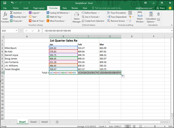
FIGURE 9-1: Rather than type repetitive formulas over and over again, Excel can copy a formula but automatically change the cell references.
From Figure 9-1, you can see that cell B10 contains the formula =B3+B4+B5+B6+B7+B8+B9, which simply adds the numbers stored in the five cells directly above the cell that contains the formula (B10). If you copy this formula to another cell, that new formula will also add the eight cells directly above it. Copy and paste this formula to cell C10, and Excel changes the formula to =C3+C4+C5+C6+C7+C8+C9.
To copy and paste a formula so that each formula changes cell references automatically, follow these steps:
- Select the cell that contains the formula you want to copy.
-
Press Ctrl+C (or click the Copy icon under the Home tab).
Excel displays a dotted line around your selected cell.
-
Select the cell (or cells) where you want to paste your formula.
If you select multiple cells, Excel pastes a copy of your formula in each of those cells. -
Press Ctrl+V (or click the Paste icon under the Home tab).
Excel pastes your formula and automatically changes the cell references.
- Press Esc or double-click away from the cell with the dotted line to make the dotted line go away.
Using Functions
Creating simple formulas is easy, but creating complex formulas is hard. To make complex formulas easier to create, Excel comes with prebuilt formulas called functions. Table 9-3 lists some common functions available.
TABLE 9-3 Common Excel Functions
|
Function Name |
What It Does |
|
AVERAGE |
Calculates the average value of numbers stored in two or more cells |
|
COUNT |
Counts how many cells contain a number instead of a label (text) |
|
MAX |
Finds the largest number stored in two or more cells |
|
MIN |
Finds the smallest number stored in two or more cells |
|
ROUND |
Rounds a decimal number to a specific number of digits |
|
SQRT |
Calculates the square root of a number |
|
SUM |
Adds the values stored in two or more cells |
Excel provides hundreds of functions that you can use by themselves or as part of your own formulas. A function typically uses one or more cell references:
- Single cell references such as
=ROUND(C4,2), which rounds the number found in cell C4 to two decimal places. - Contiguous (adjacent) cell ranges such as
=SUM(A4:A9), which adds all the numbers found in cells A4, A5, A6, A7, A8, and A9. - Noncontiguous cell ranges such as
=SUM(A4,B7,C11), which adds all the numbers found in cells A4, B7, and C11.
To use a function, follow these steps:
- Click in the cell where you want to create a formula using a function.
- Click the Formulas tab.
-
Click one of the following function icons in the Function Library group:
- Financial: Calculates business-related equations, such as the amount of interest earned over a specified time period.
- Logical: Provides logical operators to manipulate True and False (also known as Boolean) values.
- Text: Searches and manipulates text.
- Date & Time: Provides date and time information.
- Lookup & Reference: Provides information about cells, such as their row headings.
- Math & Trig: Offers mathematical equations.
- More Functions: Provides access to statistical and engineering functions.
The Recently Used icon displays a list of functions you’ve used in the past. -
Click a function category, such as Financial or Math & Trig.
A pull-down menu appears, as shown in Figure 9-2.
-
Click a function.
The Function Arguments dialog box appears, as shown in Figure 9-3.
- Click the cell references you want to use.
- Repeat Step 6 as many times as necessary.
-
Click OK.
Excel displays the calculation of your function in the cell you selected in Step 1.

FIGURE 9-2: Clicking a function library icon displays a menu of available functions you can use.

FIGURE 9-3: Specify which cell references contain the data your function needs to calculate a result.
Using the AutoSum command
One of the most useful and commonly used commands is the AutoSum command. The AutoSum command uses the SUM function to add two or more cell references without making you type those cell references yourself. The most common use for the AutoSum function is to add a column or row of numbers.
To add a column or row of numbers with the AutoSum function, follow these steps:
- Create a column or row of numbers that you want to add.
- Click at the bottom of the column or the right of the row.
- Click the Formulas tab.
-
Click the AutoSum icon in the Function Library group.
Excel automatically creates a SUM function in the cell you chose in Step 2 and highlights all the cells where it will retrieve data to add, as shown in Figure 9-4. (If you accidentally click the downward-pointing arrow under the AutoSum icon, a pull-down menu appears. Just choose Sum.)
-
Press Enter.
Excel automatically sums all the cell references.

FIGURE 9-4: The AutoSum command automatically creates cell references for the SUM function.
The AutoSum icon also appears on the Home tab in the Editing group. You can also press Alt+= to choose AutoSum, too.
Using recently used functions
Digging through all the different function library menus can be cumbersome, so Excel tries to make your life easier by creating a special Recently Used list that contains (what else?) a list of the functions you’ve used most often. From this menu, you can see just a list of your favorite functions and ignore the other hundred functions that you may never need in a million years.
To use the list of recently used functions, follow these steps:
- Click in the cell where you want to store a function.
- Click the Formulas tab.
-
Click the Recently Used icon in the Function Library group.
A pull-down menu appears, as shown in Figure 9-5.
- Choose a function.

FIGURE 9-5: The Recently Used menu lists the functions you’ve used most often.
The more functions you use, the more your list will vary from what you see in Figure 9-5.
Editing a Formula
After you create a formula, you can always edit it later. You can edit a formula in two places:
- In the Formula bar
- In the cell itself
To edit a formula in the Formula bar, follow these steps:
-
Select the cell that contains the formula you want to edit.
Excel displays the formula in the Formula bar.
- Click in the Formula bar and edit your formula by using the Backspace and Delete keys.
To edit a formula in the cell itself, follow these steps:
-
Double-click in the cell that contains the formula you want to edit.
Excel displays a cursor in the cell you select.
- Edit your formula by using the Backspace and Delete keys.
Because formulas display their calculations in a cell, it can be hard to tell the difference between cells that contain numbers and cells that contain formulas. To make formulas visible, press Ctrl+` (an accent grave character, which appears on the same key as the tilde, the ~ symbol).
Conditional Formatting
A formula in a cell can display a variety of values, depending on the data that the formula receives. Because a formula can display any type of a number, you may want to use conditional formatting as a way to highlight certain types of values.
Suppose you have a formula that calculates your monthly profits. You can change the formatting to emphasize the results:
- If your result is zero or a loss, display that value in red.
- If you make a profit under $1,000, display that value in yellow.
- If the profit is at least $100,000, display that value in green.
Conditional formatting simply displays data in a formula in various ways, depending on the value that the formula calculates.
Comparing data values
The simplest type of conditional formatting displays different colors or icons based on adjacent values, which makes it easy to compare different numbers at a glance.
Excel offers three types of conditional formatting for identifying values, as shown in Figure 9-6:
- Data Bars: Higher values display more color while lower values display less color.
- Color Scales: Different colors identify different ranges of values.
- Icon Sets: Different icons identify different ranges of values.

FIGURE 9-6: Conditional formatting can identify values of different cells.
To apply conditional formatting, follow these steps:
- Select the cells that you want to apply conditional formatting.
-
Click the Home tab and then click the Conditional Formatting icon in the Styles group.
A menu appears (refer to Figure 9-6).
-
Move the mouse over Data Bars, Color Scales, or Icon Sets.
A menu appears.
-
Click the type of conditional formatting you want.
Excel applies your conditional formatting over the cells you chose in Step 1.
Creating conditional formatting rules
Using colors or icons to identify ranges of values may be nice, but you may want to define your own rules for how conditional formatting should work, such as displaying all negative values in red and all values above 1,000 in green.
To define your own rules for formatting values, follow these steps:
- Select the cells that you want to apply conditional formatting.
-
Click the Home tab and then click the Conditional Formatting icon in the Styles group.
A menu appears (refer to Figure 9-6).
-
Move the mouse over Highlight Cells Rules.
A menu appears, as shown in Figure 9-7.
-
Click an option such as Greater Than or Between.
A dialog box appears, which lets you define one or more values and choose a color for formatting your selected cells, as shown in Figure 9-8.
-
Type a value, choose a color for formatting, and click OK.
Excel displays conditional formatting only to those selected cells that meet the criteria you define.

FIGURE 9-7: The Highlight Cells Rules displays a variety of options.

FIGURE 9-8: A dialog box lets you define a value and color to format cells.
If you click the Conditional Formatting icon on the Home tab and choose Top/Bottom Rules, Excel can apply conditional formatting to your top (or bottom) ten values or those values above or below the average, as shown in Figure 9-9.
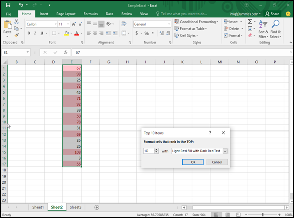
FIGURE 9-9: The Top/Bottom Rules menu can identify the top/bottom values or those above/below the average.
Data Validation
Because formulas are only as accurate as the data they receive, it’s important that your spreadsheet contains only valid data. Examples of invalid data may be a negative number (such as –9) for a price or a decimal number (such as 4.39) for the number of items a customer bought.
To keep your spreadsheet from accepting invalid data, you can define a cell to accept only certain types of data, such as numbers that fall between 30 and 100. The moment someone tries to type invalid data into a cell, Excel immediately warns you, as shown in Figure 9-10.

FIGURE 9-10: Excel warns you if you type invalid data in a cell.
To define valid types of data for a cell, follow these steps:
- Click in a cell that contains data used by a formula.
- Click the Data tab.
-
Click the Data Validation icon in the Data Tools group.
The Data Validation dialog box appears, as shown in Figure 9-11.
If you click the downward-pointing arrow that appears to the right of the Data Validation icon, a menu appears. Choose Data Validation to open the Data Validation dialog box. -
Click the Allow list box and choose one of the following:
- Any Value: The default value accepts anything the user types.
- Whole Number: Accepts only whole numbers, such as 47 and 903.
- Decimal: Accepts whole and decimal numbers, such as 48.01 or 1.00.
- List: Allows you to define a list of valid data.
- Date: Accepts only dates.
- Time: Accepts only times.
- Text length: Defines a minimum and maximum length for text.
- Custom: Allows you to define a formula to specify valid data.
Depending on the option you choose, you may need to define Minimum and Maximum values and whether you want the data to be equal to, less than, or greater than a defined limit.
- Click the Input Message tab in the Data Validation dialog box, as shown in Figure 9-12.
- Click in the Title text box and type a title.
- Click in the Input Message text box and type a message you want to display when someone selects this particular cell.
- Click the Error Alert tab in the Data Validation dialog box, as shown in Figure 9-13.
- Click the Style list box and choose an alert icon, such as Stop or Warning.
- Click in the Title text box and type a title for your error message.
- Click in the Error Message text box and type the message to appear if the user types invalid data into the cell.
- Click OK.

FIGURE 9-11: Define the type and range of acceptable data allowed in a cell.

FIGURE 9-12: The Input Message tab lets you display a message explaining the type of valid data a cell can hold.

FIGURE 9-13: Define an error message to show if the user types invalid data into the cell.
After you define data validation for a cell, you can always remove it later. To remove validation for a cell, follow these steps:
- Click in the cell that contains data validation.
- Click the Data tab.
-
Click the Data Validation icon in the Data Tools group.
The Data Validation dialog box appears (refer to Figure 9-11).
-
Click the Clear All button and then click OK.
Excel clears all your data validation rules for your chosen cell.
Goal Seeking
When you create a formula, you can type in data to see how the formula calculates a new result. However, Excel also offers a feature known as Goal Seeking. With Goal Seeking, you specify the value you want a formula to calculate, and then Excel changes the data in the formula’s cell references to tell you what values you need to achieve that goal.
For example, suppose you have a formula that calculates how much money you make every month by selling a product such as cars. Change the number of cars you sell, and Excel calculates your monthly commission. But if you use Goal Seeking, you can specify you want to earn $5,000 for your monthly commission, and Excel will work backward to tell you how many cars you need to sell. As its name implies, Goal Seeking lets you specify a goal and see what number, in a specific cell, needs to change to help you reach your goal.
To use Goal Seeking, follow these steps:
- Click in a cell that contains a formula.
- Click the Data tab.
-
Click the What-If Analysis icon in the Forecast group.
A pull-down menu appears, as shown in Figure 9-14.
-
Click Goal Seek.
The Goal Seek dialog box appears, as shown in Figure 9-15.
- Click in the To value text box and type a number that you want to appear in the formula stored in the cell that you clicked in Step 1.
-
Click in the By Changing Cell text box and click one cell that contains data used by the formula you chose in Step 1.
Excel displays your cell reference, such as $B$5, in the Goal Seek dialog box.
-
Click OK.
The Goal Seek Status dialog box changes the data in the cell you chose in Step 6, as shown in Figure 9-16.
- Click OK (to keep the changes) or click Cancel (to display the original values your spreadsheet had before you chose the Goal Seek command).

FIGURE 9-14: The What-If Analysis icon displays the Goal Seek command.

FIGURE 9-15: Define your goal in a cell containing a formula.

FIGURE 9-16: The Goal Seek Status dialog box changes the data to reach your desired goal.
Creating Multiple Scenarios
Spreadsheets show you what happened in the past. However, you can also use a spreadsheet to help predict the future by typing in data that represents your best guess of what may happen.
When you use a spreadsheet as a prediction tool, you may create a best-case scenario (where customers flood you with orders) and a worst-case scenario (where hardly anybody buys anything). You can type in different data to represent multiple possibilities, but then you’d wipe out your old data. For a quick way to plug different data into the same spreadsheet, Excel offers scenarios.
A scenario lets you define different data for multiple cells, which creates multiple spreadsheets. That way, you can choose a scenario to plug in one set of data, and then switch back to your original data without retyping all your original data and formulas all over again.
Creating a scenario
Before you can create a scenario, you must first create a spreadsheet with data and formulas. Then you can create a scenario to define the data to plug into one or more cells.
To create a scenario, follow these steps:
- Click the Data tab.
-
Click the What-If Analysis icon in the Forecast group.
A pull-down menu appears.
-
Click Scenario Manager.
The Scenario Manager dialog box appears.
-
Click Add.
The Add Scenario dialog box appears, as shown in Figure 9-17.
- Click in the Scenario Name text box and type a descriptive name for your scenario, such as Worst-case or Best-case.
- Click in the Changing Cells text box.
- Click in a cell in your spreadsheet that you want to display different data. If you want to choose multiple cells, hold down the Ctrl key and click multiple cells.
- Click in the Comment text box and type any additional comments you want to add to your scenario, such as any assumptions your scenario made.
-
Click OK.
The Scenario Values dialog box appears, as shown in Figure 9-18.
- Type a new value for each cell.
-
Click OK.
The Scenario Manager dialog box appears, as shown in Figure 9-19.
-
Click Show.
Excel replaces any existing data with the data you typed in Step 10.
-
Click Close.
The data from your scenario remains in the spreadsheet.
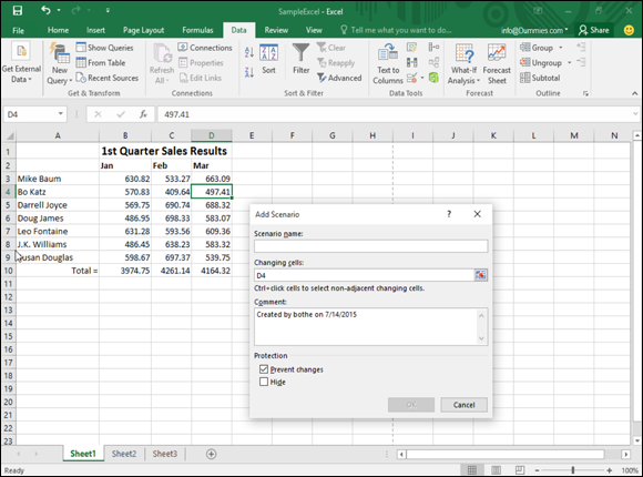
FIGURE 9-17: Define a scenario name, the cells you want to change, and any comments you want to include.

FIGURE 9-18: Type in new values for your selected cells.

FIGURE 9-19: The Scenario Manager dialog box lets you view, edit, or delete your different scenarios.
Viewing a scenario
After you create one or more scenarios, you can view them and see how they affect your data. To view a scenario, follow these steps:
- Click the Data tab.
-
Click the What-If Analysis icon in the Forecast group.
A pull-down menu appears.
-
Choose Scenario Manager.
The Scenario Manager dialog box appears (refer to Figure 9-19).
- Click the name of the scenario you want to view.
-
Click Show.
Excel shows the values in the cells defined by your chosen scenario.
- Click Close.
Editing a scenario
After you create a scenario, you can always change it later by defining new data. To edit a scenario, follow these steps:
- Click the Data tab.
-
Click the What-If Analysis icon in the Forecast group.
A pull-down menu appears.
-
Choose Scenario Manager.
The Scenario Manager dialog box appears.
-
Click the name of the scenario you want to edit and click Edit.
The Edit Scenario dialog box appears.
- (Optional) Edit the name of the scenario.
-
Click in the Changing Cells text box.
Excel displays dotted lines around all the cells that the scenario will change.
- Press Backspace to delete cells, or hold down the Ctrl key and click additional cells to include in your scenario.
-
Click OK.
The Scenario Values dialog box appears (refer to Figure 9-18).
-
Type new values for your cells and click OK when you’re done.
The Scenario Manager dialog box appears again.
- Click Show to view your scenario, or click Close to make the Scenario Manager dialog box disappear.
Viewing a scenario summary
If you have multiple scenarios, it can be hard to switch back and forth between different scenarios and still understand which numbers are changing. To help you view the numbers that change in all your scenarios, you can create a scenario summary.
A scenario summary displays your original data, along with the data stored in each scenario, in a table. By viewing a scenario summary, you can see how the values of your spreadsheet can change depending on the scenario, as shown in Figure 9-20.

FIGURE 9-20: A scenario summary compares your original data with all the data from your scenarios in an easy-to-read chart.
To create a scenario summary on a separate sheet in your workbook, follow these steps:
- Click the Data tab.
-
Click the What-If Analysis icon in the Forecast group.
A pull-down menu appears.
-
Choose Scenario Manager.
The Scenario Manager dialog box appears.
-
Click Summary.
The Scenario Summary dialog box appears, as shown in Figure 9-21.
- Select the Scenario Summary radio button.
- Click in the Result Cells text box and then click in a cell that contains a formula that your scenario affects.
-
Click OK.
Excel displays a Scenario Summary (refer to Figure 9-20).
To exit out of the Scenario Summary, just click a different sheet tab near the bottom-left corner of the Excel window.

FIGURE 9-21: Define the type of summary to create.
Auditing Your Formulas
Your spreadsheet provides results that are only as good as the data you give it and the formulas you create. Feed a spreadsheet the wrong data, and it will (obviously) calculate the wrong result. More troublesome is when you feed a spreadsheet the right data but your formula is incorrect, which produces a misleading and incorrect result.
Even if Excel appears to be calculating your formulas correctly, recheck your calculations just to make sure. Some common errors that can mess up your formulas include
- Missing data: The formula isn’t using all the data necessary to calculate the proper result.
- Incorrect data: The formula is getting data from the wrong cell (or wrong data from the right cell).
- Incorrect calculation: Your formula is incorrectly calculating a result.
If a formula is calculating data incorrectly, you probably didn’t type the formula correctly. For example, you may want a formula to add two numbers, but you accidentally typed in the formula to multiply two numbers instead. To check whether a formula is calculating data incorrectly, give it data for which you already know what the result should be. For example, if you type the numbers 4 and 7 into a formula that should add two numbers, but it returns 28 instead, you know that it’s not calculating correctly.
If your formula is correct but it’s still not calculating the right result, chances are good that it’s not getting the data it needs from the correct cells. To help you trace whether a formula is receiving all the data it needs, Excel offers auditing features that visually show you which cells supply data to which formulas. By using Excel’s auditing features, you can
- Make sure that your formulas are using data from the correct cells.
- Find out instantly whether a formula can go haywire if you change a cell reference.
Finding where a formula gets its data
If a formula is retrieving data from the wrong cells, it’s never going to calculate the right result. By tracing a formula, you can see all the cells that a formula uses to retrieve data.
Any cell that supplies data to a formula is a precedent.
To trace a formula, follow these steps:
- Click in a cell that contains the formula you want to check.
- Click the Formulas tab.
-
Click the Trace Precedents icon in the Formula Auditing group.
Excel draws arrows that show you all the cells that feed data into the formula you chose in Step 1, as shown in Figure 9-22.
- Click the Remove Arrows button to make the auditing arrows go away.

FIGURE 9-22: Excel draws arrows that trace the precedent cells that feed data into a formula.
Finding which formula(s) a cell can change
Sometimes you may be curious about how a particular cell may affect a formula stored in your worksheet. Although you can just type a new value in that cell and look for any changes, it’s easier (and more accurate) to identify all formulas that are dependent on a particular cell.
Any formula that receives data is a dependent.
To find one or more formulas that a single cell may affect, follow these steps:
- Click in any cell that contains data (not a formula).
- Click the Formulas tab.
-
Click Trace Dependents.
Excel draws an arrow that points to a cell that contains a formula, as shown in Figure 9-23. This tells you that if you change the data in the cell you chose in Step 1, it will change the calculated result in the cell containing a formula.
- Click the Remove Arrows icon in the Formula Auditing group to make the arrows go away.

FIGURE 9-23: Excel can identify which formulas a particular cell can change.
Checking for Errors
If you create large worksheets with data and formulas filling rows and columns, it can be hard to check to make sure that there aren’t any problems with your spreadsheet, such as a formula dividing a number with a nonexistent value in another cell.
Fortunately, you can get Excel to catch many types of errors by following these steps:
- Click the Formulas tab.
-
Click the left side of the Error Checking icon in the Formula Auditing group.
Excel displays a dialog box and highlights any errors, as shown in Figure 9-24.
- Click any of the options such as Previous or Next to see any additional errors.
- Click the close box in the dialog box to make it go away when you’re done using it.
- Click in a cell that contains an error.
-
Click the downward-pointing arrow that appears to the right of the Error Checking icon.
A menu appears.
-
Click Trace Error.
Excel displays arrows to show you the cells that are causing the problem for the error you chose in Step 5, as shown in Figure 9-25.
- Click the Remove Arrows icon in the Formula Auditing group to make the arrows go away.

FIGURE 9-24: Excel can identify many common errors in a spreadsheet.

FIGURE 9-25: Excel can show you where errors are occurring in your spreadsheet.