1.1 Overview of Current Situation in Methodological Aspects of Reliability Prediction

Because the problem of reliability prediction is so important there are many publications in the area of the methods of reliability prediction, mostly in the area of electronics. This is especially important when the reliability prediction is necessary to provide a high degree of effectiveness for the products.

Most of these traditional methods of reliability prediction utilize failure data collected from the field to estimate the parameters of the failure time distribution or degradation process. Using this data one can then estimate the reliability measures of interest, such as the expected time to failure or quantity/quality of degradation during a specified time interval and the mean time to failure (or degradation).

Reliability prediction models that utilize accelerated degradation data, rather than those models that utilize degradation data obtained under normal conditions, are often performed because the degradation process is very slow under normal field conditions and prediction modeling based on normal conditions would require excessive time.

One example of such practices is the procedure used by Bellcore for both hardware and software. O'Connor and Kleyner [1] provide a broad description of a reliability prediction method that emphasizes reliability prediction consisting of outputs from the reliability prediction procedure:

• steady‐state failure rate;
• first year multiplier;
• failure rate curve;
• software failure rate.

The output from the reliability prediction procedure is various estimates of how often failure occurs. With hardware, the estimates of interest are the steady‐state failure rate, the first year multiplier, and the failure rate curve. The steady‐state failure rate is a measure of how often units fail after they are more than 1 year old. The steady‐state failure rate is measured in FIT (failures per 10⁹ h of operation). A failure rate of 5000 FIT means that about 4% of the units that are over a year old will fail during following one year periods. The first year multiplier is the ratio of the failure rate in the first year to that in subsequent years. Using these, one generates a failure rate curve that provides the failure rate as a function of the age (volume of work) of the equipment. For software, one needs to know how often the system fails in the field as a result of faults in the software.

The Bellcore hardware reliability prediction is primarily designed for electronic equipment. It provides predictions at the device level, the unit level, and for simple serial systems, but it is primarily aimed at units, where units are considered nonrepairable assemblies or plug‐ins. The goal is to provide the user with information on how often units will fail and will need to be replaced.

The software prediction procedure estimates software failure intensity and applies to systems and modules.

There are many uses for reliability prediction information. One such example is, it can be used as inputs to life‐cycle cost or profit studies. Life‐cycle cost studies determine the cost of a product over its entire life. Required data include how often a unit will have to be replaced. Inputs to this process include the steady‐state failure rate and the first year multiplier.

The Bellcore reliability prediction procedure consists of three methods [1]:

1. Parts count. These predictions are based solely by adding together the failure rates for all the devices. This is the most commonly used method, because laboratory and field information that is needed for the other methods is usually not available.
2. Incorporating laboratory information. Device or unit level predictions are obtained by combining data from a laboratory test with the data from the parts count method. This allows suppliers to use their data to produce predictions of failure rates, and it is particularly suited for new devices for which little field data are available.
3. Incorporating field information. This method allows suppliers to combine field performance data with data from the parts count method to obtain reliability predictions.

Mechanical reliability prediction [2] uses various stress factors under operating conditions as a key to reliability prediction for different devices. This situation is more common in testing mechanical devices, such as bearings, compressors, pumps, and so on than with electronic hardware.

Although, the number of factors that appear to be needed in reliability testing calculations may appear excessive, tailoring methods can be used to remove factors that have little or no influence, or for which limited data are available. Generally, the problems encountered in attempting to predict the reliability of mechanical systems are the lack of:

• specific or generic failure rate data;
• information on the predominant failure modes;
• information on the factors influencing the reliability of the mechanical components.

The mechanical reliability prediction approach can be useful if there is a close connection with the source of information for calculation reliability during the desired time, whether that be warranty period, service life, or other defined period. Obtaining accurate initial information is a critical factor in prediction testing.

Unfortunately, the approaches described earlier, and other prediction methods, provide little guidance on how one can obtain accurate initial information that simulates real product reliability over time or amount of use (volume of work, or duty cycle). Without accurate simulation information, its usefulness is minimal.

Proper understanding of the role of testing and the requirement to do this testing before the production and use of a product is critical and can easily lead to poor product reliability prediction that will negatively impact financial performance.

Prediction is only useful if it reduces early product degradation and prevents premature failures of the product.

There are many recent publications addressing electronics, automotive, and other product recalls. While they usually address reliability failures in terms of safety matters that affect peoples lives by contributing to deaths or injuries, they may also consider economic impacts.

As was mentioned previously, such reliability and other problems are results, not causes. The actual causes of these recalls, and many other technical and economic problems, were a direct result of the inefficient or inadequate prediction of product reliability during the design, and prior to, the manufacturing process.

In the end, it is poorly executed prediction that negatively impacts the organizations financial performance.

Therefore, while many popular and commonly used approaches appear to be theoretically interesting, in the end they do not successfully predict reliability for the product in real‐world applications.

Consider the consequences of the recalls of Takata automobile air bag inflators [3]:

So far, about 12.5 million suspect Takata inflators have been fixed of the roughly 65 million inflators (in 42 million vehicles) that will ultimately be affected by this recall, which spans 19 automakers. Carmakers and federal officials organizing the response to this huge recall insist that the supply chain is churning out replacement parts, most of which are coming from companies other than Takata. For those who are waiting, NHTSA advises that people not disable the airbags; the exceptions are the 2001–2003 Honda and Acura models that we listed on this page on June 30, 2016—vehicles which NHTSA is telling people to drive only to a dealer to get fixed.

Meanwhile, a settlement stemming from a federal probe into criminal wrongdoing by Takata is expected early next year—perhaps as soon as January—and could approach $1 billion.

A key to preventing these situations is the use of advanced test methods and equipment; that is, accelerated reliability testing (ART) and accelerated durability testing (ADT). Implementation of these systematic procedures greatly helps in assuring successful prediction of industrial product reliability.

It is also true that advances in technology generally result in more complicated products and increased economic development costs. Such advances require even more attention to accurately predict product reliability.

When performed successfully, prediction is beneficial to all stages of the product life cycle: start‐up, production and manufacturing, warranty, and long‐term aftermarket support. It touches the lives of all concerned (designers, suppliers, manufacturers, customers), and often even uninvolved third parties who may be affected by the product's failure. It also provides the mechanism for product improvement at any time from the earliest stages of R&D throughout the entire product life cycle.

Currently there are many other publications mostly related to the theoretical aspects of reliability prediction. Many of primarily relate to failure analysis. Some popular failure analysis methods and tools include:

• Failure Reporting, Analysis, and Corrective Action System (FRACAS);
• Failure Mode, Effects and Critical Analysis (FMECA);
• Failure Mode and Effects Analysis (FMEA);
• Fault Tree Analysis (FTA).

FavoWeb is Advanced Logistic Developments' (ADL's) third‐generation, web‐based and user‐configurable FRACAS that captures information about equipment or the processes throughout its life cycle, from design, through to production, testing, and customer support.

FavoWeb has been adopted by world‐class organizations who, for the first time ever, implement a FRACAS application that seamlessly communicates with any given enterprise resource planning (ERP) system (SAP, ORACLE, MFGpro, etc.), while proving a user‐friendly and flexible, yet robust, failure management, analysis, and corrective action platform.

The FavoWeb FRACAS features include:

• full web‐base application;
• user permission mechanism—complies with International Traffic in Arms Regulations requirements;
• flexible, user configurable application;
• seamless communication with ERP/product data management/Excel/Access and other legacy systems;
• web services infrastructure;
• failure/event chaining and routing;
• compatible with PDAs;
• voice‐enabled failure reporting;
• advanced query engine for user‐defined reports.

It also allows the user to decompose the system or process into components or subprocesses. And, for each functional block, it allows the user to define name and function, and enter failure mode causes and effects manually or from libraries. The “Process & Design FMEA” module provides full graphical and textual visibility of the potential failure mode → cause → effects chain.

1.1.3 Classical Test Theory

The goal of reliability theory is to estimate errors in measurement and to suggest ways of improving tests so that these errors are minimized. The central assumption of reliability theory is that measurement errors are essentially random. This does not mean that errors arise from random processes. For any individual, an error in measurement is not a completely random event. However, across a large number of individuals, the causes of measurement error are assumed to be so varied that measure errors act as random variables. If errors have the essential characteristics of random variables, then it is reasonable to assume that errors are equally likely to be positive or negative, and that they are not correlated with true scores or with errors on other tests.

Unfortunately, there is no way to directly observe or calculate the true score, so a variety of methods are used to estimate the reliability of a test. Some examples of the methods used to estimate reliability include test–retest reliability, internal consistency reliability, and parallel‐test reliability. Each method approaches the problem of accounting for the source of error in the test somewhat differently.

1.1.6 About Reliability Software

The reliability software modules of the ITEM ToolKit [7] provide a user‐friendly interface that allows one to construct, analyze, and display system models using the module's interactive facilities. Building hierarchies and adding new components could not be easier. ToolKit calculates the failure rates, including mean time between failures (MTBFs), associated with new components as they are added to the system, along with the overall system failure rate. Project data may be viewed via grid view and dialog view simultaneously, allowing predictions to be performed with a minimum of effort.

Each reliability prediction module is designed to analyze and calculate component, subsystem, and system failure rates in accordance with the appropriate standard. After the analysis is complete, ITEM ToolKit's integrated environment comes into its own with powerful conversion facilities to transfer data to other reliability software modules. For example, you can transfer your MIL‐217 project data to FMECA or your Bellcore project to RBD. These powerful features transfer as much of the available information as possible, saving valuable time and effort [7].

The following is an interesting statement from ReliaSoft's analysis of the current situation in reliability prediction [8]:

To obtain high product reliability, consideration of reliability issues should be integrated from the very beginning of the design phase. This leads to the concept of reliability prediction. The objective of reliability prediction is not limited to predicting whether reliability goals, such as MTBF, can be reached. It can also be used for:

• Identifying potential design weaknesses
• Evaluating the feasibility of a design
• Comparing different designs and life‐cycle costs
• Providing models statement from system reliability/availability analysis
• Aiding in business decisions such as budget allocation and scheduling

Once the product's prototype is available, lab tests can be utilized to obtain reliability predictions. Accurate prediction of the reliability of electronic products requires knowledge of the components, the design, the manufacturing process and the expected operating conditions. Several different approaches have been developed to achieve reliability prediction of electronic systems and components. Each approach has its advantages and disadvantages. Among these approaches, three main categories are often used within government and industry:

• empirical (standard bases);
• physics of failure, and;
• life testing.

The following provides an overview of all three approaches [8].

1.1.6.1 MIL‐HDBK‐217 Predictive Method

MIL‐HDBK‐217 is very well known in military and commercial industries. Version MIL‐HDBK‐217F was released in 1991 and had two revisions.

The MIL‐HDBK‐217 predictive method consists of two parts: one is known as the parts count method and the other is called the part stress method [8]. The parts count method assumes typical operating conditions of part complexity, ambient temperature, various electrical stresses, operation mode, and environment (called reference conditions). The failure rate for a part under the reference conditions is calculated as

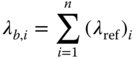
where λ _ref is the failure rate under the reference conditions and i is the number of parts.

Since the parts may not operate under the reference conditions, the real operating conditions may result in failure rates different than those given by the “parts count” method. Therefore, the part stress method requires the specific part's complexity, application stresses, environmental factors, and so on. These adjustments are called Pi factors. For example, MIL‐HDBK‐217 provides many environmental conditions, expressed as π _E, ranging from “ground benign” to “cannon launch.” The standard also provides multilevel quality specifications that are expressed as π _Q. The failure rate for parts under specific operating conditions can be calculated as

where π _S is the stress factor, π _T is the temperature factor, π _E is the environment factor, π _Q is the quality factor, and π _A is the adjustment factor.

1.1.6.2 Bellcore/Telcordia Predictive Method

Bellcore was a telecommunication research and development company that provided joint R&D and standards setting for AT&T and its co‐owners. Bellcore was not satisfied with the military handbook methods for application with their commercial products, so Bellcore designed its own reliability prediction standard for commercial telecommunication products. Later, the company was acquired by Science Applications International Corporation (SAIC) and the company's name was changed to Telcordia. Telcordia continues to revise and update the Bellcore standard. Presently, there are two updates: SR‐332 Issue 2 (September 2006) and SR‐332 Issue 3 (January 2011), both titled “Reliability prediction procedure for electronic equipment.”

The Bellcore/Telcordia standard assumes a serial model for electronic parts and it addresses failure rates at both the infant mortality stage and at the steady‐state stages utilizing Methods I, II, and III. Method I is similar to the MIL‐HDBK‐217F parts count and part stress methods, providing the generic failure rates and three part stress factors: device quality factor π _Q, electrical stress factor π _S, and temperature stress factor π _T. Method II is based on combining Method I predictions with data from laboratory tests performed in accordance with specific SR‐332 criteria. Method III is a statistical prediction of failure rate based on field tracking data collected in accordance with specific SR‐332 criteria. In Method III, the predicted failure rate is a weighted average of the generic steady‐state failure rate and the field failure rate.

1.1.6.3 Discussion of Empirical Methods

Although empirical prediction standards have been used for many years, it is wise to use them with caution. The advantages and disadvantages of empirical methods have been discussed, and a brief summary from publications in industry, military, and academia is presented next [8].

Advantages of empirical methods:

1. Easy to use, and a lot of component models exist.
2. Relatively good performance as indicators of inherent reliability.

Disadvantages of empirical methods:

1. Much of the data used by the traditional models is out of date.
2. Failure of the components is not always due to component‐intrinsic mechanisms, but can be caused by the system design.
3. The reliability prediction models are based on industry‐average values of failure rate, which are neither vendor specific nor device specific.
4. It is hard to collect good‐quality field and manufacturing data, which are needed to define the adjustment factors, such as the Pi factors in MIL‐HDBK‐217.

1.1.7 Physics of Failure Methods

In contrast to empirical reliability prediction methods that are based on the statistical analysis of historical failure data, a physics of failure approach is based on the understanding of the failure mechanism and applying the physics of failure model to the data. Several popularly used models are discussed next.

1.1.7.1 Arrhenius's Law

One of the earliest acceleration models predicts how the time to failure of a system varies with temperature. This empirically based model is known as the Arrhenius equation. Generally, chemical reactions can be accelerated by increasing the system temperature. Since it is a chemical process, the aging of a capacitor (such as an electrolytic capacitor) is accelerated by increasing the operating temperature. The model takes the following form:

where L(T) is the life characteristic related to temperature, A is a scaling factor, E _a is the activation energy, k is the Boltzmann constant, and T is the temperature.

1.1.7.2 Eyring and Other Models

While the Arrhenius model emphasizes the dependency of reactions on temperature, the Eyring model is commonly used for demonstrating the dependency of reactions on stress factors other than temperature, such as mechanical stress, humidity, or voltage. The standard equation for the Eyring model [8] is as follows:

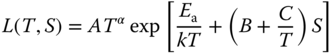
where L(T,S) is the life characteristic related to temperature and another stress, A, α, B, and C are constants, S is a stress factor other than temperature, and T is absolute temperature.

According to different physics of failure mechanisms, one more factor (i.e., stress) can be either removed or added to the standard Eyring model. Several models are similar to the standard Eyring model.

Electronic devices with aluminum or aluminum alloy with small percentages of copper and silicon metallization are subject to corrosion failures and therefore can be described with the following model [8]:

where B ₀ is an arbitrary scale factor, α is equal to 0.1 to 0.15 per %RH, and f(V) is an unknown function of applied voltage, with an empirical value of 0.12–0.15.

1.1.7.3 Hot Carrier Injection Model

Hot carrier injection describes the phenomena observed in metal–oxide–semiconductor field‐effect transistors (MOSFETs) by which the carrier gains sufficient energy to be injected into the gate oxide, generate interface or bulk oxide defects, and degrade MOSFET characteristics such as threshold voltage, transconductance, and so on [8].

For n‐channel devices, the model is given by

where B is an arbitrary scale factor, I _sub is the peak substrate current during stressing, N is equal to a value from 2 to 4 (typically 3), and E _a is equal to −0.1 to −0.2 eV.

For p‐channel devices, the model is given by:

where B is an arbitrary scale factor, I _gate is the peak gate current during stressing, M is equal to a value from 2 to 4, and E _a is equal to −0.1 to −0.2 eV.

ReliaSoft's “Reliability prediction methods for electronic products” [8] states:

Since electronic products usually have a long time period of useful life (i.e., the constant line of the bathtub curve) and can often be modeled using an exponential distribution, the life characteristics in the above physics of failure models can be replaced by MTBF (i.e., the life characteristic in the exponential distribution). However, if you think your products do not exhibit a constant failure rate and therefore cannot be described by an exponential distribution, the life characteristic usually will not be the MTBF. For example, for the Weibull distribution, the life characteristic is the scale parameter eta and for the lognormal distribution, it is the log mean.

1.1.7.4 Black Model for Electromigration

Electromigration is a failure mechanism that results from the transfer of momentum from the electrons, which move in the applied electric field, to the ions, which make up the lattice of the interconnect material. The most common failure mode is “conductor open.” With the decreased structure of integrated circuits (ICs), the increased current density makes this failure mechanism very important in IC reliability.

At the end of the 1960s, J. R. Black developed an empirical model to estimate the mean time to failure (MTTF) of a wire, taking electromigration into consideration, which is now generally known as the Black model. The Black model employs external heating and increased current density and is given by

where A ₀ is a constant based on the cross‐sectional area of the interconnect, J is the current density, J _threshold is the threshold current density, E _a is the activation energy, k is the Boltzmann constant, T is the temperature, and N is a scaling factor.

The current density J and temperature T are factors in the design process that affect electromigration. Numerous experiments with different stress conditions have been reported in the literature, where the values have been reported in the range between 2 and 3.3 for N, and 0.5 to 1.1 eV for E _a. Usually, the lower the values, the more conservative the estimation.

1.1.7.5 Discussion of Physics of Failure Methods

A given electronic component will have multiple failure modes, and the component's failure rate is equal to the sum of the failure rates of all modes (i.e., humidity, voltage, temperature, thermal cycling, and so on). The authors of this method propose that the system's failure rate is equal to the sum of the failure rates of the components involved. In using the aforementioned models, the model parameters can be determined from the design specifications or operating conditions. If the parameters cannot be determined without conducting a test, the failure data obtained from the test can be used to get the model parameters. Software products such as ReliaSoft's ALTA can help analyze the failure data; for example, to analyze the Arrhenius model. For this example, the life of an electronic component is considered to be affected by temperature. The component is tested under temperatures of 406, 416, and 426 K. The usage temperature level is 400 K. The Arrhenius model and the Weibull distribution are used to analyze the failure data in ALTA.

Advantages of physics of failure methods:

1. Modeling of potential failure mechanisms based on the physics of failure.
2. During the design process, the variability of each design parameter can be determined.

Disadvantages of physics of failure methods:

1. The testing conditions do not accurately simulate the field conditions.
2. There is a need for detailed component manufacturing information, such as material, process, and design data.
3. Analysis is complex and could be costly to apply.
4. It is difficult (almost impossible) to assess the entire system.

Owing to these limitations, this is not generally a practical methodology.

1.2 Current Situation in Practical Reliability Prediction

There are far fewer publications that relate to the practical aspects of reliability prediction. Sometimes authors call their publications by some name indicating practical reliability prediction, but the approaches they present are not generally useful in a practical way.

The electronics community is comprised of representatives from electronics suppliers, system integrators, and the Department of Defense (DoD). The majority of the reliability work is driven by the user community that depends heavily on solid reliability data. BAE Systems, Bechtel, Boeing, General Dynamics, Harris, Lockheed Martin, Honeywell, Northrop Grumman, and Raytheon are some of the better known demand‐side contributors to the work done by the reliability community. These members have developed consensus documents to define electronics failure rate prediction methodologies and standards. Their efforts have produced a series of documents that have been ANSI and VITA ratified. In some cases, these standards provide adjustment factors to existing standards.

The reliability community addresses some of the limitations of traditional prediction practices with a series of subsidiary specifications that contain “best practices” within the industry for performing electronics failure rate predictions. The members recognize that there are many industry reliability methods, each with a custodian and a methodology of acceptable practices, to calculate electronics failure rate predictions. If additional standards are required, for use by electronics module suppliers, a new subsidiary specification will be considered by the working group.

ANSI/VITA 51.3 Qualification and Environmental Stress Screening in Support of Reliability Predictions provides information on how qualification levels and environmental stress screening may be used to influence reliability.

Although they sometimes call what are essentially empirical prediction methods “practical methods”, these approaches do not provide accurate and successful prediction during the product's service life. Let us briefly review these and some other relevant publications.

David Nicholls provides an overview in this area [41]:

• For more than 25 years, there has been a passionate dialog throughout the reliability engineering community as to the appropriate use of empirical and physics‐based reliability models and their associated benefits, limitations, and risks.
• Over its history, the Reliability Information Analysis Center has been intimately involved in this debate. It has developed models for MIL‐HDBK‐217, as well as alternative empirically based methodologies such as 217Plus. It has published books related to physics‐of‐failure modeling approaches and developed the Web‐Accessible Repository for Physics‐based Models to support the use of physics‐of‐failure approaches. In DoD‐sponsored documents it also had published ideal attributes to identify future reliability predicting methods.
• Empirical predicting methods, particularly those based on field data, provide average failure rates based on the complexities of actual environmental and operational stresses. Generally, they should be used only in the absence of actual relevant comparison data. They are frequently criticized, however, for being grossly inaccurate in prediction of actual field failure rates, and for being used and accepted primarily for verification of contractual reliability requirements.
• What should your response be (if protocol allows) if you are prohibited from using one prediction approach over another because it is claimed that, historically, those prediction methods are “inaccurate,” or they are deemed too labor intensive/cost ineffective to perform based on past experience?
• Note that the terms “predicting,” “assessment,” and “estimation” are not always distinguishable in the literature.
• A significant mistake typically made in comparing actual field reliability data with the original prediction is that the connection is lost between the root failure causes experienced in the field and the intended purpose/coverage of the reliability prediction approach. For example, MIL‐HDBK‐217 addresses only electronic and electromechanical components. Field failures whose root failure cause is traced to mechanical components, software, manufacturing deficiencies, and so on, should not be scored against a MIL‐HDBK‐217 prediction.
• Data that form the basis for either an empirical or physics‐based prediction has various factors that will influence any uncertainty in the assessments made using the data. One of the most important factors is relevancy. Relevancy is defined as the similarity between the predicted and fielded product/system architectures, complexities, technologies, and environmental/operational stresses.
• Empirical reliability prediction models based on field data inherently address all of the failure mechanisms associated with reliability in the field, either explicitly (e.g., factors based on temperature) or implicitly (generic environmental factors that “cover” all of the failure mechanisms not addressed explicitly). They do not, however, assess or consider the impact of these various mechanisms on specific failure modes, nor do they (generally) consider “end‐of‐life” issues.
• The additional insight required to ensure an objective interpretation of results for physics‐based prediction includes:
  • What failure mechanisms/modes of interest are addressed by the predicting?
  • What are the reliability or safety risks associated with the failure mechanisms/modes not addressed by the prediction?
  • Does the prediction consider interactions between failure mechanisms (e.g., combined maximum vibration level and minimum temperature level).

As a result of the overview, Nicholls concluded:

1. As the reader may have noticed, there was one question brought up in the paper that was never addressed: “How can one ensure that prediction results will not be misinterpreted or misapplied, even though all assumptions and rationale have been meticulously documented and clearly stated?”
2. Unfortunately, the answer is: “You can't.” Regardless of the care taken to ensure a technically valid and supportable analysis, empirical and physics‐based predicting will always need to be justified as to why the predicted reliability does not reflect the measured reliability in the field.

From the aforementioned information we can conclude that current prediction methods in engineering are primarily related to computer science, and even there they are not entirely successful. Given this fact, how much less is known about prediction, especially accurate prediction, that relates to automotive, aerospace, aircraft, off‐highway, farm machinery, and others? We need to conclude that it is even less developed in these areas.

A fatigue life prediction method for practical engineering use was proposed by Theil [42]:

• According to this method, the influence of overload events can be taken in account.
• The validation was done using uniaxial tests carried out on metallic specimens.

It is generally accepted that during a product's service life high load cycles will occur in addition to the normally encountered operational loads. Therefore, the development of an accurate fatigue life prediction rule which takes into account overloads in the vicinity of and slightly above yield strength, with a minimal level of effort for use in practical engineering at the design stress level, would still be highly significant.

Theil's paper [42] presents a fatigue life prediction method based on an S/N curve for constant‐amplitude loading. Similarities and differences between the proposed method and the linear cumulative damage rule of Pålmgren–Miner are briefly discussed. Using the method presented, an interpretation of the Pålmgren–Miner rule from the physical point of view is given and clarified with the aid of a practical two‐block loading example problem.

Unfortunately however, statistical reliability predictions rarely correlate with field performance. The basic cause is that they are based on testing methods that incorrectly simulate the real‐world interacted conditions.

Therefore, similar to the contents of Section 1.1, current practical reliability prediction approaches cannot provide industry with with the necessary or appropriate tools to dramatically increase reliability, eliminate (or dramatically reduce) recalls, complaints, costs, and other technical and economic aspects of improved product performance.

1.3 From History of Reliability Prediction Development

The term “reliability prediction” has historically been used to denote the process of applying mathematical models and data for the purpose of estimating the field reliability of a system before empirical data are available for the system [43,44].

Jones [45] considered information on the history of reliability prediction allowing his work to be placed in context with general developments in the field. This includes the development of statistical models for lifetime prediction using early life data (i.e., prognostics), the use of nonconstant failure rates for reliability prediction, the use of neural networks for reliability prediction, the use of artificial intelligence systems to support reliability engineers' decision‐making, the use of a holistic approach to reliability, the use of complex discrete events simulation to model equipment availability, the demonstration of the weaknesses of classical reliability prediction, an understanding of the basic behavior of no fault founds, the development of a parametric drift model, the identification of the use of a reliability database to improve the reliability of systems, and an understanding of the issues that surround the use of new reliability metrics in the aerospace industry.

During World War II, electronic tubes were by far the most unreliable component used in electronic systems. This observation led to various studies and ad hoc groups whose purpose was to identify ways that electronic tube reliability, and the reliability of the systems in which they operated, could be improved. One group in the early 1950s concluded that:

1. There needed to be better reliability‐data collected from the field.
2. Better components needed to be developed.
3. Quantitative reliability requirements needed to be established.
4. Reliability needed to be verified by test before full‐scale production.

The specification requirement to have quantitative reliability requirements in turn led to the need to have a means of estimating reliability before the equipment is built and tested so that the probability of achieving its reliability goal could be estimated. This was the beginning of reliability prediction.

Then, in the 1960s, the first version of US MH‐217 was published by the US Navy. This document became the standard by which reliability predictions were performed. Other sources of failure rates prediction gradually disappeared. These early sources of failure‐rate predicting often included design guidance on the reliable application of electronic components.

In the early 1970s, the responsibility for preparing MH‐217 was transferred to the Rome Air Development Center, who published revision B in 1974. While this MH‐217 update reflected the technology at that time, there were few other efforts to change the manner in which predicting was performed. And these efforts were criticized by the user community as being too complex, too costly, and unrealistic.

While MH‐217 was updated several times, in the 1980s other agencies were developing reliability predicting models unique to their industries. For example, the SAE Reliability Standard Committee developed a set of models specific to automotive electronics. The SAE committee did this because it was their belief that there were no existing prediction methodologies that applied to the specific quality levels and environments appropriate for automotive applications.

The Bellcore reliability‐prediction standard is another example of a specific industry developing methodologies for their unique conditions and equipment. But regardless of the developed methodology, the conflict between the usability of a model and its accuracy has always been a difficult compromise.

In the 1990s, much of the literature on reliability prediction centered around whether the reliability discipline should focus on physics‐of‐failure‐based or empirically based models (such as MH‐217) for the qualification of reliability.

Another key development in reliability prediction related to the effects of acquisition reform, which overhauled the military standardization process. These reforms in turn led to a list of standardization documents that required priority action, because they were identified as barriers to commercial acquisition processes, as well as major cost drivers in defense acquisitions.

The premise of traditional methods, such as MH‐217, is that the failure rate is primarily determined by components comprising the system. The prediction methodologies that were developed toward the end of the 1990s had the following advantages:

• they used all available information to form the best estimate of field reliability;
• they were tailorable;
• they had quantifiable statistical‐confidence bounds;
• they had sensitivity to the predominant system‐reliability drivers.

During this time, some reliability professionals believed that reliability modeling should focus more on physics‐of‐failure models to replace the traditional empirical models. Physics‐of‐failure models attempt to model failure mechanisms deterministically, as opposed to the traditional approach of using models based on empirical data.

Physics‐of‐failure techniques can be effective for estimating lifetimes due to specific failure mechanisms. These techniques are useful for ensuring that there are no quantifiable failure mechanisms that will occur in a given time period. However, many of the arguments that physics‐of‐failure proponents use are based on erroneous assumptions regarding empirically based reliability prediction. The fact that a failure rate can be predicted for a given part under a specific set of conditions does not imply that a failure rate is an inherent quality of a part.

Rather, the probability of failure is a complex interaction between the defect density, defect severity, and stresses incurred in operation. Failure rates predicted using empirical models are therefore typical failure rates and represent typical defect rates, design, and use conditions.

Therefore, there is a tradeoff between the model's usability and its required level of detailed data. This highlights the fact that the purpose of a reliability prediction must be clearly understood before a methodology is chosen.

From the foregoing we can conclude that current prediction methods in engineering mostly relate to computer science, and even they are not very successful. And as relates to prediction (especially successful prediction) of automotive, aircraft, off‐highway, farm machinery, and others, we need to accept that prediction methods are even less developed.

A similar conclusion was made by Wong [46]:

Inaccurate reliability predictions could lead to disasters such as in the case of the U.S. Space Shuttle failure. The question is: ‘what is wrong with the existing reliability prediction methods?’ This paper examines the methods for predicting reliability of electronics. Based on information in the literature the measured vs predicted reliability could be as far apart as five to twenty times. Reliability calculated using the five most commonly used handbooks showed that there could be a 100 times variation. The root cause for the prediction inaccuracy is that many of the first‐order effect factors are not explicitly included in the prediction methods. These factors include thermal cycling, temperature change rate, mechanical shock, vibration, power on/off, supplier quality difference, reliability improvement with respect to calendar years, and ageing. As indicated in the data provided in this paper, any one of these factors neglected could cause a variation in the predicted reliability by several times. The reliability vs ageing‐hour curve showed that there was a 10 times change in reliability from 1000 ageing‐hours to 10,000 ageing‐hours. Therefore, in order to increase the accuracy of reliability prediction the factors must be incorporated into the prediction methods.

1.4 Why Reliability Prediction is Not Effectively Utilized in Industry

As one can see from Figure 1.1, reliability is a result of many interacting components which influence the product's performance. Therefore, one needs to understand that, if we consider reliability separately, it is different from that in the real‐life situation. Reliability prediction is only one aspect that is a result of the interacted product performance in real life (i.e., only one step of product/technology performance). Klyatis [30] gives full consideration of product performance prediction.

As was previously discussed, there are many methodological approaches to different aspects of engineering prediction; these include Refs [47–59], but there are many other publications on the subject.

The problems remain:

• How can one obtain common methodological (strategic and tactical) aspects of interacted components performance for successful prediction? Reliability is only one of many interacted factors of a product's or a technology's performance (Figure 1.1).
• How does one obtain accurate initial information necessary for each particular product's successful performance prediction, including reliability, safety, durability, life cycle cost, and others?

In order to solve these problems, one needs to understand the basic causes of why the approaches used until now cannot solve problems of successfully predicting reliability.

One frequently encountered cause is that the management structure of many large and middle‐size companies is hierarchical, with managerial responsibilities that provide no, or inadequate, interconnections or interactions with other areas of the organization, or with outside entities supplying components or services to their companies.

Too often this leads to parochial thinking and inadequate consideration of how other sections of their organization influence their product's effectiveness. Figure 1.2 demonstrates sectors of responsibility of four vice presidents (1, 2, 3, 4) in a large organization. Each vice‐president's sector of responsibility consists of some subsectors, shown as subsectors 3a, 3b, and 3c, each with a corresponding responsible technical director, or some similar title (example in Figure 1.2). These subsector directors do not communicate enough with each other, because each sub‐director's responsibility relates to their particular subsector only. But their work interacts and influences the final reliability of the product.

Let us consider some examples from author's practice. After reading author's publications, Mr. Takashi Shibayama, Vice President of Jatco Ltd (Japan) (design and manufacturing for automobile transmissions), indicated that he was very interested in implementing these practices at Jatco Ltd. Mr. Shibayama came to the SAE World Congress bringing his copy of author's book Accelerated Reliability and Durability Testing Technology, published by Wiley, which he had studied. After discussion with Dr. Klyatis, Mr. Shibayama and Jatco's engineers and managers returned to Japan and asked by e‐mail if I could meet with Nissan management. It was agreed that a meeting would be scheduled during the next SAE World Congress in Detroit. This meeting would be attended by leaders in the Powertrain Engineering Division at Nissan. Mr. Shibayama indicated these people would all be the expert leaders in Nissan reporting directly to the highest levels in Nissan.

One participant was from the Engine Department, and another from the Drive Train Department, one was the engineering director involved directly in human factor problems, and another the engineering director in engine problems. They first attended author's presentation at the SAE 2013 World Congress, Technical Session IDM300 Trends in Development Accelerated Reliability and Durability Testing, as well as author's “Chat with the Expert” session. The company's personnel had studied his book, Accelerated Reliability and Durability Testing Technology, prior to the meeting. During the meeting, they asked if he would help them to improve each of their separate areas for reliability, and he replied that he could not. The reason for this answer was that each of them was responsible for their specific area and they did not interact with the other areas of Nissan's engineering. He said that all sectors and components of the vehicle interact and are interconnected, and if we consider each component separately then you could not hope to obtain a successful improvement in prediction. He pointed out that page 65 in his book emphasized the need for solving reliability issues in a complex product, and that as long as each area of the business worked independently, overall product reliability prediction could not be improved.

From discussions with other industrial companies' managements, as well as reviewing their work, it became evident that similar situations are prevalent in other areas of industry, including, for example, the aircraft industry.

Figure 1.3 is provided as an aid in understanding why the current discussions in Sections 1.1 and 1.2 fail to provide accurate information for successful reliability prediction. A short description of the basic causes depicted in Figure 1.3 follows:

1. Reliability and durability evaluation results are usually provided directly after stress testing either in the laboratory or from proving grounds testing. This evaluation only relates to the test conditions (the laboratory or proving ground testing). But in order to know the test subject's reliability or durability in actual use, the laboratory or proving ground testing results are not adequate, as field use normally entails probabilistic, random (often nonstationary) characteristics that require more complicated methods than evaluation based on laboratory (with simple simulation of the field) or proving ground test protocols. But, this more complex methodology is seldom used. As a result, simpler evaluation methods are used, but these are not reliable predictors.
2. Typical testing is performed for several separate parameters, such as vibration or temperature, with allowances possibly including a few others. But in real‐world operation there are many other factors influencing or affecting the test subject. Temperature, humidity, air pollution (mechanical and chemical), radiation (visible, ultraviolet, and infrared), air fluctuation, features of the road (type of road, profile, density, etc.), speed of movement, input voltage, electrostatic discharge, and other factors may be present in different combinations. If laboratory or proving grounds simulations use only several of the multi‐environmental real‐world input influences described here, this ignores what may well be significant interactions between different factors that will influence reliability and durability. This is one reason why current accelerated stress testing fails to accurately predict the reliability and durability of the product, whether it be components or the completed product in the field.
3. Often, companies' suppliers use only components (details) and assemblies (units) stress testing, ignoring the interconnections between these components and assemblies. Therefore, the stress testing results are different from the test subject's results in the real world. These results cannot help to predict accurately the reliability and durability of the product in the field.
4. A basic reason for many product recalls is inaccurate simulation and mistakes in using stress testing results, which lead to inaccurate prediction of a product's reliability. The result is that an organization's profit is reduced from that which was projected or potentially could have been achieved. As Kanapady and Adib noted [22], “Money was saved years earlier by gambling with a substandard reliability program, but the short‐term gain was not a good long‐term investment.”
5. In an attempt to compensate for unknown field factors, companies sometimes use accelerated stress testing with loads greater than maximum field loads. This alters the physics‐of‐degradation or the chemistry‐of‐degradation process obtained in actual field use. As a result, the time and character to failures, as well as the number and cost of failures, during this testing can be different from the failures in the field situation.
6. As each failure mechanism responds to stress differently, and each component of the product has several different failure mechanisms, using accelerated test data plus a single acceleration factor can result in a time between failures (MTBF) estimate that is erroneous and misleading [37].
7. There is no standard stress stimulus portfolio. Because of the vast diversity of products, each product and program will have differences. This is often forgotten.
8. Reliability assumptions based on statistically determined sample sizes are often invalid, because the samples rarely are truly random representations of production parts.
9. Often, the parameters used for field loading simulation for stress testing are not based on the truly representative region, and do not represents all areas (including climatic) of the product's use in the field.
10. Some accelerated testing uses simulation at constant stress, or step stress, or cycling stress that contradicts the real‐world situation, where loading has a random stress nature.
11. As Wong noted [46], inaccurate reliability predictions could lead to disasters, such as in the case of the US Space Shuttle failure. The question is: “What is wrong with the existing reliability prediction methods?” This textbook answers this question.

These are some of the reasons, why current accelerated stress testing does not help accurately predict reliability and durability. But these limitations can be reduced or eliminated by switching to ART and ADT. Descriptions of these types of testing can be found in the literature [30,60–66]. These publications provide guidance on how to accurately simulate the field situation for obtaining initial information for accurate reliability development and prediction.

For successful ART/ADT technology implementation, a multidisciplinary team will be needed to manage and engineer the application of this technology to a particular product. The team should include, as a minimum, the following:

• A team leader who is both a high‐level manager and who also understands the strategy of this technology. The team leader must understand the principles of accurate simulation of the field situation, and what other professional disciplines need to be included in the team.
• A program manager to act as a guide throughout the process and who can remove any barriers that prevent the team from succeeding. The program manager must also be knowledgeable in the design and technology of both the product and the testing.
• Engineering resources to actually perform much of the testing. This includes selection of appropriate candidate test units, failure analysis, chemical problems solution in simulation, physical problems solution in simulation, prediction methodology, system of control development, design, diagnostic, and corrective action for mechanical, electrical, hydraulic, and so on, as well as both hardware and software development and implementation.

The team must work closely with those departments that are responsible for design, manufacturing, marketing, and selling the product.

References

1. 1 O'Connor P, Kleyner A. (2012). Practical Reliability Engineering, 5th edition. John Wiley & Sons.
2. 2 Naval Surface Warfare Center, Carderock Division. (2011). Handbook of Reliability Prediction Procedures for Mechanical Equipment. Logistic Technology Support, Carderockdiv, NSWC‐10. West Naval Surface Warfare Center, Carderock Division, Bethesda, MD.
3. 3 Atiyeh C, Blackwell R. (2016). Massive Takata airbag recall: everything you need to know, including full list of affected vehicles. Update: December 29. Car and Driver. https://blog.caranddriver.com/massive‐takata‐airbag‐recall‐everything‐you‐need‐to‐know‐including‐full‐list‐of‐affected‐vehicles/ (accessed January 18, 2018).
4. 4 National Council on Measurement in Education. (2017). Glossary of important assessment and measurement terms. http://www.ncme.org/ncme/NCME/Resource_Center/Glossary/NCME/Resource_Center/Glossary1.aspx?hkey=4bb87415‐44dc‐4088‐9ed9‐e8515326a061#anchorR (accessed January 18, 2018).
5. 5 Carlson NR. Miller HL Jr, Heth DS, Donahoe JW, Martin GN. (2009). Psychology: The Science of Behaviour, 4th Canadian edn. Pearson, Toronto.
6. 6 Web Center for Social Research Methods. (2006). Types of reliability, in The Research Methods Knowledge Base. https://www.socialresearchmethods.net/kb/reltypes.php (accessed January 18, 2018).
7. 7 Weibull.com (2005). Standards based reliability prediction: applicability and usage to augment RBDs. Part I: introduction to standards based reliability prediction and lambda predict. Reliability HotWire Issue 50 (April). http://www.weibull.com/hotwire/issue50/hottopics50.htm (accessed January 18, 2018).
8. 8 ReliaSoft. Reliability prediction methods for electronic products. Reliability EDGE 9(1). http://www.reliasoft.com/pubs/reliabilityedge_v9i1.pdf (accessed January 18, 2018).
9. 9 ANSI/VITA 51.2 (2016). Physics of Failure Reliability Predictions.
10. 10 Blischke WR, Prabhakar Murthy DN. (2000). Reliability: Modeling, Prediction, and Optimization. John Wiley & Sons.
11. 11 Wiley Online Library. (2000). Short Book Reviews, 20(3).
12. 12 Misra KB. (1992). Reliability Analysis and Prediction, Volume 15. A Methodology Oriented Treatment. Elsevier Science.
13. 13 Jones TL (2010). Handbook of Reliability Prediction Procedures for Mechanical Equipment. Naval Surface Warfare Center, Carderock Division.
14. 14 An YH, Draughn RA. (1999). Mechanical Testing of Bone–Implant Interface. CRC Press.
15. 15 European Power Supply Manufacturers Association. (2005). Guidelines to understanding reliability prediction. http://wwwepsma.org/MTBF%20Report_24%20June%202005.pdf (accessed January 18, 2018).
16. 16 Gipper J. (2014). Choice of Reliability Prediction Methods. http://vita.mil‐embedded.com/articles/choice‐reliability‐prediction‐methods/ (accessed February 2, 2018).
17. 17 Cai Y‐K, Wei D, Ma X‐B, Zhao Y. Reliability prediction method with field environment variation. In 2015 Annual Reliability and Maintainability Symposium (RAMS). IEEE Press, pp. 1–7.
18. 18 Chigurupati A, Thibaux R, Lassar N. (2016). Predicting hardware failure using machine learning. In 2016 Annual Reliability and Maintainability Symposium (RAMS). IEEE Press, pp. 1–6.
19. 19 Wang Q, Chen D, Bai H. (2016). A method of space radiation environment reliability prediction. In 2016 Annual Reliability and Maintainability Symposium (RAMS). IEEE Press, pp. 1–6.
20. 20 Wang L, Zhao X, Wang X, Mu M. (2016). A lifetime prediction method with hierarchical degradation data. In 2016 Annual Reliability and Maintainability Symposium (RAMS). IEEE Press, pp. 1–6.
21. 21 Jakob F, Schweizer V, Bertsche B, Dobry A. (2014). Comprehensive approach for the reliability prediction of complex systems. In 2014 Reliability and Maintainability Symposium. IEEE Press, pp. 1–6.
22. 22 Kanapady R, Adib R. Superior reliability prediction in design and development phase. In 2013 Proceedings Annual Reliability and Maintainability Symposium (RAMS). IEEE Press, pp. 1–6.
23. 23 Hava A, Qin J, Bernstein JB, Bo Y. Integrated circuit reliability prediction based on physics‐of‐failure models in conjunction with field study. In 2013 Proceedings Annual Reliability and Maintainability Symposium (RAMS). IEEE Press, pp. 1–6.
24. 24 Thaduri A, Verma AK, Gopika V, Kumar U. Reliability prediction of constant fraction discriminator using modified PoF approach. In 2013 Proceedings Annual Reliability and Maintainability Symposium (RAMS). IEEE Press, pp. 1–7.
25. 25 Thaduri A, Verma AK, Kumar U. Comparison of reliability prediction methods using life cycle cost analysis. In 2013 Proceedings Annual Reliability and Maintainability Symposium (RAMS). IEEE Press, pp. 1–7.
26. 26 DAU. (1995). MIL‐HDBK‐217F (Notice 2). Military Handbook: Reliability Prediction of Electronic Equipment. Department of Defense, Washington, DC.
27. 27 Telecordia. (2016). SR‐332, Issue 4, Reliability Prediction Procedure for Electronic Equipment.
28. 28 Lu H, Kolarik WJ, Lu SS. (2001). Real‐time performance reliability prediction. IEEE Transactions on Reliability 50(4): 353–357.
29. 29 NIST/SEMATECH. (2010). Assessing product reliability. In Engineering Statistics e‐Handbook. US Department of Commerce, Washington, DC, chapter 8.
30. 30 Klyatis L. (2016) Successful Prediction of Product Performance: Quality, Reliability, Durability, Safety, Maintainability, Life‐Cycle Cost, Profit, and Other Components. SAE International, Warrendale, PA.
31. 31 DAU. (1991). MIL‐HDBK‐217F (Notice 1). Military Handbook: Reliability Prediction of Electronic Equipment. Department of Defense, Washington, DC.
32. 32 Telcordia. (2001). SR‐332, Issue 1, Reliability Prediction Procedure for Electronic Equipment.
33. 33 Telcordia. (2006). SR‐332, Issue 2, Reliability Prediction Procedure for Electronic Equipment.
34. 34 ITEM Software and ReliaSoft Corporation. (2015). D490 Course Notes: Introduction to Standards Based Reliability Prediction and Lambda Predict.
35. 35 Foucher B, Boullie J, Meslet B, Das D. (2002). A review of reliability prediction methods for electronic devices. Microelectronics Reliability 42(8): 1155–1162.
36. 36 Pecht M, Das D, Ramarkrishnan A. (2002). The IEEE standards on reliability program and reliability prediction methods for electronic equipment. Microelectronics Reliability 42: 1259–1266.
37. 37 Talmor M, Arueti S. (1997). Reliability prediction: the turnover point. In Annual Reliability and Maintainability Symposium: 1997 Proceedings. IEEE Press, pp. 254–262.
38. 38 Hirschmann D, Tissen D, Schroder S, de Doncker RW. (2007). Reliability prediction for inverters in hybrid electrical vehicles. IEEE Transactions on Power Electronics, 22(6): 2511–2517.
39. 39 NIST Information Technology Library. https://www.itl.nist.gov.
40. 40 SeMaTech International. (2000) Semiconductor Device Reliability Failure Models. www.sematech.org/docubase/document/3955axfr.pdf (accessed January 19, 2018).
41. 41 Nicholls D. An objective look at predictions – ask questions, challenge answers. In 2012 Proceedings Annual Reliability and Maintainability Symposium. IEEE Press, pp. 1–6.
42. 42 Theil N. (2016). Fatigue life prediction method for the practical engineering use taking in account the effect of the overload blocks. International Journal of Fatigue 90: 23–35.
43. 43 Denson W. (1998). The history of reliability prediction. IEEE Transactions on Reliability 47(3‐SP, Part 2): SP‐321–SP‐328.
44. 44 Klyatis L. The role of accurate simulation of real world conditions and ART/ADT technology for accurate efficiency predicting of the product/process. In SAE 2014 World Congress, paper 2014‐01‐0746.
45. 45 Jones JA. (2008). Electronic reliability prediction: a study over 25 years. PhD thesis, University of Warwick.
46. 46 Wong KL. (1990). What is wrong with the existing reliability prediction methods? Quality and Reliability Engineering International 6(4): 251–257.
47. 47 Black AI. (1989). Bellcore system hardware reliability prediction. In Proceedings Annual Reliability and Maintainability Symposium.
48. 48 Bowles JB. (1992). A survey of reliability prediction procedures for microelectronic devices. IEEE Transactions in Reliability 41: 2–12.
49. 49 Chan HT, Healy JD. (1985). Bellcore reliability prediction. In Proceedings Annual Reliability and Maintainability Symposium.
50. 50 Healy JD, Aridaman KJ, Bennet JM. (1999). Reliability prediction. In Proceedings Annual Reliability and Maintainability Symposium.
51. 51 Leonard CT, Recht M. (1990). How failure prediction methodology affects electronic equipment design. Quality and Reliability Engineering International 6: 243–249.
52. 52 Wymysłowski A. (2011). Editorial. 2010 EuroSimE international conference on thermal, mechanical and multi‐physics simulation and experiments in micro‐electronics and micro‐systems. Microelectronics Reliability 51: 1024–1025.
53. 53 Kulkarni C, Biswas G, Koutsoukos X. (2010). Physics of failure models for capacitor degradation in DC–DC converters. https://c3.nasa.gov/dashlink/static/media/publication/2010_MARCON_DCDCConverter.pdf (accessed January 19, 2018).
54. 54 Eaton DH, Durrant N, Huber SJ, Blish R, Lycoudes N. (2000). Knowledge‐based reliability qualification testing of silicon devices. International SEMATECH Technology Transfer # 00053958A‐XFR. http://www.sematech.org/docubase/document/3958axfr.pdf (accessed January 19, 2018).
55. 55 Osterwald CR, McMahon TJ, del Cueto JA, Adelstein J, Pruett J. (2003). Accelerated stress testing of thin‐film modules with SnO₂:F transparent conductors. Presented at the National Center for Photovoltaics and Solar Program Review Meeting Denver , Colorado. https://www.nrel.gov/docs/fy03osti/33567.pdf (accessed January 19, 2018).
56. 56 Vassiliou P, Mettas A. (2003). Understanding accelerated life‐testing analysis. In 2003 Annual Reliability and Maintainability Symposium.
57. 57 Mettas A. (2010). Modeling and analysis for multiple stress‐type accelerated life data. In 46th Reliability and Maintainability Symposium.
58. 58 Dodson B, Schwab H. (2006). Accelerated Testing: A Practitioner's Guide to Accelerated and Reliability Testing. SAE International, Warrendale, PA.
59. 59 Ireson WG, Combs CF Jr, Moss RY. (1996). Handbook on Reliability Engineering and Management. McGraw‐Hill.
60. 60 Klyatis LM, Klyatis EL. (2006). Accelerated Quality and Reliability Solutions. Elsevier.
61. 61 Klyatis LM, Klyatis EL. (2002). Successful Accelerated Testing. Mir Collection, New York.
62. 62 Klyatis LM, Verbitsky D. Accelerated Reliability/Durability Testing as a Key Factor for Accelerated Development and Improvement of Product/Process Reliability, Durability, and Maintainability. SAE Paper 2010‐01‐0203. Detroit. 04/12/2010. (Also in the book SP‐2272).
63. 63 Klyatis L. (2009). Specifics of accelerated reliability testing. In IEEE Workshop Accelerated Stress Testing. Reliability (ASTR 2009) [CD], October 7–9, Jersey City.
64. 64 Klyatis L, Vaysman A. (2007/2008). Accurate simulation of human factors and reliability, maintainability, and supportability solutions. The Journal of Reliability, Maintainability, Supportability in Systems Engineering (Winter).
65. 65 Klyatis L. (2006). Elimination of the basic reasons for inaccurate RMS predictions. In A Governmental–Industry Conference “RMS in A Systems Engineering Environment”, DAU‐West, San Diego, CA, October 11–12.
66. 66 Klyatis LM. (2012). Accelerated Reliability and Durability Testing Technology. John Wiley & Sons, Inc., Hoboken, NJ.

Exercises

1. 1.1 List three currently used traditional methods of reliability prediction.
2. 1.2 Briefly describe the concept of the basic methods in Example 1.1.
3. 1.3 Why are these methods mostly theoretical?
4. 1.4 Why do most publications in reliability prediction relate to electronics?
5. 1.5 Why are most approaches to reliability prediction of a theoretical nature?
6. 1.6 What is the description of classical test theory?
7. 1.7 What is the basic approach of the Bellcore/Telecordia prediction method?
8. 1.8 What is the basic approach of the MIL‐HDBK‐17 predictive method?
9. 1.9 What is the basic approach of the ReliaSoft analysis in reliability prediction?
10. 1.10 Describe some of the advantages and disadvantages of empirical methods of reliability prediction.
11. 1.11 Describe the basic concept of the physics‐of‐failure method of reliability prediction.
12. 1.12 What factors does the Black model for electromigration in electronic products add to reliability prediction modeling?
13. 1.13 What is the basic content of the reliability software modules of the ITEM Toolkit?
14. 1.14 What is the background for the reliability prediction as used by Bellcore for hardware and software?
15. 1.15 What are some of the software and hardware prediction procedures used by Bellcore?
16. 1.16 What procedures are used when employing the Bellcore reliability prediction procedure?
17. 1.17 What problems are encountered with attempts to predict product reliability of mechanical systems using the Handbook of Reliability Prediction Procedures of Mechanical Equipment?
18. 1.18 What is the real cause of many recalls?
19. 1.19 What are the basic methods of failure analysis?
20. 1.20 Give a short description of the methods you gave in Exercise 1.19.
21. 1.21 What are the general classes of reliability estimates?
22. 1.22 What are some of the major factors in general model reliability prediction?
23. 1.23 What are the basic strategies of estimating reliability methods?
24. 1.24 Describe some of the advantages and disadvantages of using standards‐based reliability prediction.
25. 1.25 Describe some of the advantages and disadvantages of using the physics‐of‐failure methods.
26. 1.26 What is the reliability factor projected by the life testing method?
27. 1.27 Why are traditional approaches to reliability prediction not successful in industrial practice?
28. 1.28 Why should accurate reliability prediction be so important to a company's management?
29. 1.29 Give some of the reasons traditional methods of reliability prediction in electronics have not been successful?
30. 1.30 Provide a short overview of both qualitative and quantitative aspects of reliability, and their differences.
31. 1.31 Provide a short synopsis of any nine of the articles on reliability prediction from the Reliability and Maintainability Symposium (RAMS) Proceedings that have been discussed in this chapter.
32. 1.32 What are some of the key elements of the Telecordia reliability prediction procedure?
33. 1.33 What is the basic meaning of the Bayesian approach to reliability prediction?
34. 1.34 List several of the basic causes for why traditional solutions using theoretical aspects of reliability prediction are not successful in industrial applications of reliability prediction.
35. 1.35 What is David Nicholls's key conclusion in his published overview of reliability prediction methods?
36. 1.36 Why is fatigue life not an accurate prediction method for successful reliability prediction?
37. 1.37 Describe the basic history of reliability prediction methods.
38. 1.38 Why are most traditional prediction methods related to computer science and manufacture?
39. 1.39 What is the problem with using separate testing aspects to make engineering predictions?
40. 1.40 Why are most presently used approaches failing to produce successful product reliability predictions?
41. 1.41 Describe some of the performance components that interact and affect reliability.
42. 1.42 Why does currently used accelerated stress testing not obtain accurate needed information for successful reliability prediction? Describe some of these causes and their potential effects on prediction.