Chapter 5
Differentials and differentiability
1 INTRODUCTION
Let us consider a function f : S → ℝm, defined on a set S in ℝn with values in ℝm. If m = 1, the function is called real‐valued (and we shall use ϕ instead of f to emphasize this); if m ≥ 2, f is called a vector function. Examples of vector functions are
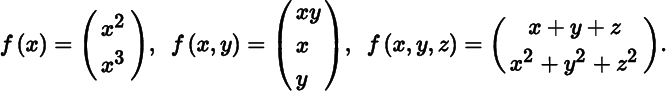
Note that m may be larger or smaller or equal to n. In the first example, n = 1, m = 2, in the second n = 2, m = 3, and in the third n = 3, m = 2.
In this chapter, we extend the one‐dimensional theory of differential calculus (concerning real‐valued functions ϕ : ℝ → ℝ) to functions from ℝn to ℝm. The extension from real‐valued functions of one variable to real‐valued functions of several variables is far more significant than the extension from real‐valued functions to vector functions. Indeed, for most purposes a vector function can be viewed as a vector of m real‐valued functions. Yet, as we shall see shortly, there are good reasons to study vector functions.
Throughout this chapter, and indeed, throughout this book, we shall emphasize the fundamental idea of a differential rather than that of a derivative as this has large practical and theoretical advantages.
2 CONTINUITY
We first review the concept of continuity. Intuitively, a function f is continuous at a point c if f(x) can be made arbitrarily close to f(c) by taking x sufficiently close to c; in other words, if points close to c are mapped by f into points close to f(c).
Definition 5.1 is a straightforward generalization of the definition in Section 4.7 concerning continuity of real‐valued functions (m = 1). Note that f has to be defined at the point c in order to be continuous at c. Some authors require that c is an accumulation point of S, but this is not assumed here. If c is an isolated point of S (a point of S which is not an accumulation point of S), then every f defined at c will be continuous at c because for sufficiently small δ there is only one point c + u in S satisfying ∥u∥ < δ, namely the point c itself, so that
If c is an accumulation point of S, the definition of continuity implies that
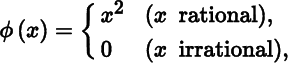
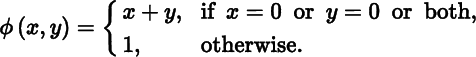
Geometrical intuition suggests that if f : S → ℝm is continuous at c, it must also be continuous near c. This intuition is wrong for two reasons. First, the point c may be an isolated point of S, in which case there exists a neighborhood of c where f is not even defined. Second, even if c is an accumulation point of S, it may be that every neighborhood of c contains points of S at which f is not continuous. For example, the real‐valued function ϕ : ℝ → ℝ defined by
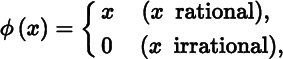
is continuous at x = 0, but at no other point.
If f : S → ℝm, the formula
defines m real‐valued functions fi : S → ℝ (i = 1, … , m). These functions are called the component functions of f and we write
If c is an accumulation point of a set S in ℝn and f : S → ℝm is continuous at c, then we can write (1) as
where
We may call Equation (2) the Taylor formula of order zero. It says that continuity at an accumulation point of S and ‘zero‐order approximation’ (approximation of f(c + u) by a polynomial of degree zero, that is a constant) are equivalent properties. In the next section, we discuss the equivalence of differentiability and first‐order (that is linear) approximation.
Exercises
- 1. Prove Theorem 5.1.
- 2. Let S be a set in ℝn. If f : S → ℝm and g : S → ℝm are continuous on S, then so is the function f + g : S → ℝm.
- 3. Let S be a set in ℝn and T a set in ℝm. Suppose that g : S → ℝm and f : T → ℝp are continuous on S and T, respectively, and that g(x) ∈ T when x ∈ S. Then the composite function h : S → ℝp defined by h(x) = f(g(x)) is continuous on S.
- 4. Let S be a set in ℝn. If the real‐valued functions ϕ : S → ℝ, ψ : S → ℝ and χ : S → ℝ − {0} are continuous on S, then so are the real‐valued functions ϕψ : S → ℝ and ϕ/χ : S → ℝ.
- 5. Let ϕ : (0, 1) → ℝ be defined by
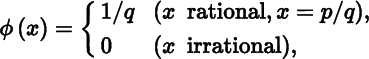
where p, q ∈ ℕ have no common factor. Show that ϕ is continuous at every irrational point and discontinuous at every rational point.
3 DIFFERENTIABILITY AND LINEAR APPROXIMATION
In the one‐dimensional case, the equation
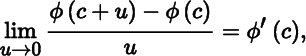
defining the derivative at c, is equivalent to the equation
where the remainder rc(u) is of smaller order than u as u → 0, that is,
Equation (4) is called the first‐order Taylor formula. If for the moment we think of the point c as fixed and the increment u as variable, then the increment of the function, that is the quantity ϕ(c + u) − ϕ(c), consists of two terms, namely a part uϕ′(c) which is proportional to u and an ‘error’ which can be made as small as we please relative to u by making u itself small enough. Thus, the smaller the interval about the point c which we consider, the more accurately is the function ϕ(c + u) — which is a function of u — represented by its affine part ϕ(c) + uϕ′(c). We now define the expression
as the (first) differential of ϕ at c with increment u.
The notation dϕ(c; u) rather than dϕ(c, u) emphasizes the different roles of c and u. The first point, c, must be a point where ϕ′(c) exists, whereas the second point, u, is an arbitrary point in ℝ.
Although the concept of differential is as a rule only used when u is small, there is in principle no need to restrict u in any way. In particular, the differential dϕ(c; u) is a number which has nothing to do with infinitely small quantities.
The differential dϕ(c; u) is thus the linear part of the increment ϕ(c + u) − ϕ(c). This is expressed geometrically by replacing the curve at point c by its tangent; see Figure 5.1.
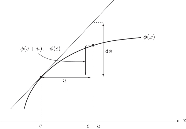
Figure 5.1 Geometrical interpretation of the differential
Conversely, if there exists a quantity α, depending on c but not on u, such that
where r(u)/u tends to 0 with u, that is if we can approximate ϕ(c + u) by an affine function (in u) such that the difference between the function and the approximation function vanishes to a higher order than the increment u, then ϕ is differentiable at c. The quantity α must then be the derivative ϕ′(c). We see this immediately if we rewrite (7) in the form
and then let u tend to 0. Differentiability of a function and the possibility of approximating a function by means of an affine function are therefore equivalent properties.
4 THE DIFFERENTIAL OF A VECTOR FUNCTION
These ideas can be extended in a perfectly natural way to vector functions of two or more variables.
In other words, f is differentiable at the point c if f(c + u) can be approximated by an affine function of u. Note that a function f can only be differentiated at an interior point or on an open set.
Since r(u, v)/(u2 + v2)1/2 → 0 as (u, v) → (0, 0), ϕ is differentiable at every point of ℝ2 and its derivative is (y2, 2xy), a row vector.
We have seen before (Section 5.2) that a function can be continuous at a point c, but fails to be continuous at points near c; indeed, the function may not even exist near c. If a function is differentiable at c, then it must exist in a neighborhood of c, but the function need not be differentiable or continuous in that neighborhood. For example, the real‐valued function ϕ : ℝ → ℝ defined by
is differentiable (and continuous) at x = 0, but neither differentiable nor continuous at any other point.
Let us return to Equation (9). It consists of m equations,
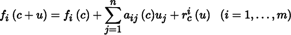
with
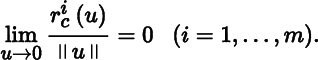
Hence, we obtain our next theorem.
In view of Theorems 5.1 and 5.2, it is not surprising to find that many of the theorems on continuity and differentiation that are valid for real‐valued functions remain valid for vector functions. It appears, therefore, that we need only study real‐valued functions. This is not so, however, because in practical applications real‐valued functions are often expressed in terms of vector functions (and indeed, matrix functions). Another reason for studying vector functions, rather than merely real‐valued functions, is to obtain a meaningful chain rule (Section 5.12).
If f : S → ℝm, S ⊂ ℝn, is differentiable on an open subset E of S, there must exist real‐valued functions aij : E → ℝ(i = 1, … , m; j = 1, … , n) such that (9) holds for every point of E. We have, however, no guarantee that, for given f, any such function aij exists. We shall prove later (Section 5.10) that, when f is suitably restricted, the functions aij exist. But first we prove that, if such functions exist, they are unique.
Exercise
- 1.
Let f : S → ℝm and g : S → ℝm be differentiable at a point c ∈ S ⊂ ℝn. Then the function h = f + g is differentiable at c with
dh(c; u) =df(c; u) +dg(c; u).
5 UNIQUENESS OF THE DIFFERENTIAL
6 CONTINUITY OF DIFFERENTIABLE FUNCTIONS
Next, we prove that the existence of the differential df(c; u) implies continuity of f at c. In other words, that continuity is a necessary condition for differentiability.
The converse of Theorem 5.4 is, of course, false. For example, the function ϕ : ℝ → ℝ defined by the equation ϕ(x) = |x| is continuous but not differentiable at 0.
Exercise
- 1.
Let ϕ : S → ℝ be a real‐valued function defined on a set S in ℝn and differentiable at an interior point c of S. Show that (i) there exists a nonnegative number M, depending on c but not on u, such that |
dϕ(c; u)| ≤ M ||u||; (ii) there exists a positive number η, again depending on c but not on u, such that |rc(u)| <∥u∥ for all u ≠ 0 with ∥u∥ < η. Conclude that (iii) |ϕ(c + u) − ϕ(c)| < (1 + M)∥u∥ for all u ≠ 0 with ∥u∥ < η. A function with this property is said to satisfy a Lipschitz condition at c. Of course, if ϕ satisfies a Lipschitz condition at c, then it must be continuous at c.
7 PARTIAL DERIVATIVES
Before we develop the theory of differentials any further, we introduce an important concept in multivariable calculus, the partial derivative.
Let f : S → ℝm be a function defined on a set S in ℝn with values in ℝm, and let fi : S → ℝ(i = 1, … , m) be the ith component function of f. Let c be an interior point of S, and let ej be the jth elementary vector in ℝn, that is the vector whose jth component is one and whose remaining components are zero. Consider another point c + tej in ℝn, all of whose components except the jth are the same as those of c. Since c is an interior point of S, c + tej is, for small enough t, also a point of S. Now consider the limit
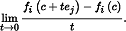
When this limit exists, it is called the partial derivative of fi with respect to the jth coordinate (or the jth partial derivative of fi) at c and is denoted by Djfi(c). (Other notations include [∂fi(x)/∂xj]x=c or even ∂fi(c)/∂xj.) Partial differentiation thus produces, from a given function fi, n further functions D1fi, …, Dnfi defined at those points in S where the corresponding limits exist.
In fact, the concept of partial differentiation reduces the discussion of real‐valued functions of several variables to the one‐dimensional case. We are merely treating fi as a function of one variable at a time. Thus, Djfi is the derivative of fi with respect to the jth variable, holding the other variables fixed.
The converse of Theorem 5.5 is false. Indeed, the existence of the partial derivatives with respect to each variable separately does not even imply continuity in all the variables simultaneously (although it does imply continuity in each variable separately, by Theorem 5.4). Consider the following example of a function of two variables:
This function is clearly not continuous at (0, 0), but the partial derivatives D1ϕ(0, 0) and D2ϕ (0, 0) both exist. In fact,
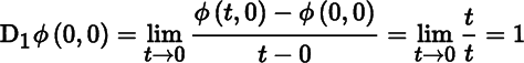
and, similarly, D2ϕ(0, 0) = 1.
A partial converse of Theorem 5.5 exists, however (Theorem 5.7).
Exercise
- 1.
Show in the example given by (16) that
D1ϕ andD2ϕ, while existing at (0, 0), are not continuous there, and that every disc B(0) contains points where the partials both exist and points where the partials both do not exist.
8 THE FIRST IDENTIFICATION THEOREM
If f is differentiable at c, then a matrix A(c) exists such that for all ∥u∥ < r,
where rc(u)/∥u∥ → 0 as u → 0. The proof of Theorem 5.5 reveals that the elements aij(c) of the matrix A(c) are, in fact, precisely the partial derivatives Djfi(c). This, in conjunction with the uniqueness theorem (Theorem 5.3), establishes the following central result.
The m × n matrix Df(c) in (17), whose ijth element is Djfi(c), is called the Jacobian matrix of f at c. It is defined at each point where the partials Djfi(i = 1, …, m; j = 1, …, n) exist. (Hence, the Jacobian matrix Df(c) may exist even when the function f is not differentiable at c.) When m = n, the absolute value of the determinant of the Jacobian matrix of f is called the Jacobian of f. The transpose of the m × n Jacobian matrix Df(c) is an n × m matrix called the gradient of f at c; it is denoted by ∇f(c). (The symbol ∇ is pronounced ‘del’.) Thus,
In particular, when m = 1, the vector function f : S → ℝm specializes to a real‐valued function ϕ : S → ℝ, the Jacobian matrix specializes to a 1× n row vector Dϕ(c), and the gradient specializes to an n × 1 column vector ∇ϕ(c).
The first identification theorem will be used throughout this book. Its great practical value lies in the fact that if f is differentiable at c and we have found a differential df at c, then the value of the partials at c can be immediately determined.
Some caution is required when interpreting Equation (17). The right‐hand side of (17) exists if (and only if) all the partial derivatives Djfi(c) exist. But this does not mean that the differential df(c; u) exists if all partials exist. We know that df(c; u) exists if and only if f is differentiable at c (Section 5.4). We also know from Theorem 5.5 that the existence of all the partials is a necessary but not a sufficient condition for differentiability. Hence, Equation (17) is only valid when f is differentiable at c.
9 EXISTENCE OF THE DIFFERENTIAL, I
So far we have derived some theorems concerning differentials on the assumption that the differential exists, or, what is the same, that the function is differentiable. We have seen (Section 5.7) that the existence of all partial derivatives at a point is necessary but not sufficient for differentiability (in fact, it is not even sufficient for continuity).
What, then, is a sufficient condition for differentiability at a point? Before we answer this question, we pose four preliminary questions in order to gain further insight into the properties of differentiable functions.
- (i) If f is differentiable at c, does it follow that each of the partials is continuous at c?
- (ii) If each of the partials is continuous at c, does it follow that f is differentiable at c?
- (iii) If f is differentiable at c, does it follow that each of the partials exists in some n‐ball B(c)?
- (iv) If each of the partials exists in some n‐ball B(c), does it follow that f is differentiable at c?
The answer to all four questions is, in general, ‘No’. Let us see why.
10 EXISTENCE OF THE DIFFERENTIAL, II
Examples 5.2–5.5 show that neither the continuity of all partial derivatives at a point c nor the existence of all partial derivatives in some n‐ball B(c) is, in general, a sufficient condition for differentiability. With this knowledge, the reader can now appreciate the following theorem.
Exercises
- 1. Prove Equation (21).
- 2. Show that, in fact, only the existence of all the partials and continuity of all but one of them is sufficient for differentiability.
- 3.
The condition that the n partials be continuous at c, although sufficient, is by no means a necessary condition for the existence of the differential at c. Consider, for example, the case where ϕ can be expressed as a sum of n functions,
ϕ(x) = ϕ1(x1) + ⋯ + ϕn(xn),
where ϕj is a function of the one‐dimensional variable xj alone. Prove that the mere existence of the partials
D1ϕ, …,Dnϕ is sufficient for the existence of the differential at c.
11 CONTINUOUS DIFFERENTIABILITY
Let f : S → ℝm be a function defined on an open set S in ℝn. If all the first‐order partial derivatives Djfi(x) exist and are continuous at every point x in S, then the function f is said to be continuously differentiable on S.
Notice that while we defined continuity and differentiability of a function at a point, continuous differentiability is only defined on an open set. In view of Theorem 5.7, continuous differentiability implies differentiability.
12 THE CHAIN RULE
A very important result is the so‐called chain rule. In one dimension, the chain rule gives a formula for differentiating a composite function h = g ° f defined by the equation
The formula states that
and thus expresses the derivative of h in terms of the derivatives of g and f. Its extension to the multivariable case is as follows.
Exercises
- 1. What is the order of the matrices A and B? Is the matrix product BA defined?
- 2. Show that the constants μA and μB in (28) exist. [Hint: Use Exercise 2 in Section 1.14.]
- 3. Write out the chain rule as a system of np equations
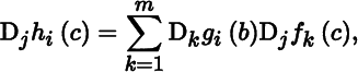
where j = 1, …, n and i = 1, …, p.
13 CAUCHY INVARIANCE
The chain rule relates the partial derivatives of a composite function h = g ○ f to the partial derivatives of g and f. We shall now discuss an immediate consequence of the chain rule, which relates the differential of h to the differentials of g and f. This result (known as Cauchy's rule of invariance) is particularly useful in performing computations with differentials.
Let h = g ○ f be a composite function, as before, such that
If f is differentiable at c and g is differentiable at b = f(c), then h is differentiable at c with
Using the chain rule, (30) becomes
We have thus proved the following.
Cauchy's rule of invariance justifies the use of a simpler notation for differentials in practical applications, which adds greatly to the ease and elegance of performing computations with differentials. We shall discuss notational matters in more detail in Section 5.16.
14 THE MEAN‐VALUE THEOREM FOR REAL‐VALUED FUNCTIONS
The mean‐value theorem for functions from ℝ to ℝ states that
for some θ ∈ (0, 1). This equation is, in general, false for vector functions. Consider for example the vector function f : ℝ → ℝ2 defined by
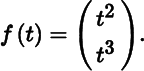
Then no value of θ ∈ (0, 1) exists such that
as can be easily verified. Several modified versions of the mean‐value theorem exist for vector functions, but here we only need the (straightforward) generalization of the one‐dimensional mean‐value theorem to real‐valued functions of two or more variables.
15 DIFFERENTIABLE MATRIX FUNCTIONS
Hitherto we have only considered vector functions. The following are examples of matrix functions:
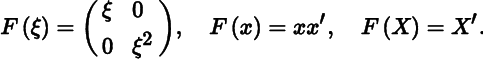
The first example maps a scalar ξ into a matrix, the second example maps a vector x into a matrix xx′, and the third example maps a matrix X into its transpose matrix X′.
To extend the calculus of vector functions to matrix functions is straight‐forward. Let us consider a matrix function F : S → ℝm × p defined on a set S in ℝn × q. That is, F maps an n × q matrix X in S into an m × p matrix F(X).
In view of Definition 5.3, all calculus properties of matrix functions follow immediately from the corresponding properties of vector functions, because instead of the matrix function F, we can consider the vector function f : vec S → ℝmp defined by
It is easy to see from (31) and (32) that the differentials of F and f are related by
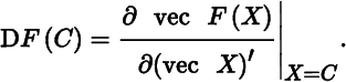
We then define the Jacobian matrix of F at C as
This is an mp × nq matrix, whose ijth element is the partial derivative of the ith component of vec F(X) with respect to the jth element of vec X, evaluated at X = C, that is,
The following three theorems are now straightforward generalizations of Theorems 5.6, 5.8, and 5.9.
Exercise
- 1. Let S be a subset of ℝn and assume that F : S → ℝm × p is continuous at an interior point c of S. Assume also that F(c) has full rank (that is, F(c) has either full column rank p or full row rank m). Prove that F(x) has locally constant rank; that is, F(x) has full rank for all x in some neighborhood of x = c.
16 SOME REMARKS ON NOTATION
We remarked in Section 5.13 that Cauchy's rule of invariance justifies the use of a simpler notation for differentials in practical applications. (In the theoretical Chapters 4–7, we shall not use this simplified notation.) Let us now see what this simplification involves and how it is justified.
Let g : ℝm → ℝp be a given differentiable vector function and consider the equation
We shall now use the symbol dy to denote the differential
In this expression, dt (previously u) denotes an arbitrary vector in ℝm, and dy denotes the corresponding vector in ℝp. Thus, dt and dy are vectors of variables.
Suppose now that the variables t1, t2, …, tm depend on certain other variables, say x1, x2, …, xn:
Substituting f(x) for t in (34), we obtain
and therefore
The double use of the symbol dy in (35) and (38) is justified by Cauchy's rule of invariance. This is easy to see, because we have, from (36),
where dx is an arbitrary vector in ℝn. Then (38) gives (by Theorem 5.9)
using (36) and (39). We conclude that Equation (35) is valid even when t1, …, tm depend on other variables x1, …, xn, although (39) shows that dt is then no longer an arbitrary vector in ℝm.
We can economize still further with notation by replacing y in (34) with g itself, thus writing (35) as
and calling dg the differential of g at t. This type of conceptually ambiguous usage (of g as both function symbol and variable) will assist practical work with differentials in Part Three.
17 COMPLEX DIFFERENTIATION
Almost all functions in this book are real‐valued. In this section, we briefly discuss differentiation of a complex‐valued function f defined on a subset of the complex plane ℂ. The function f can be expressed in terms of two realvalued functions u and v:
We can also consider u and v to be functions of two real variables x and y (rather than of one complex variable z) by writing z = x + iy, so that
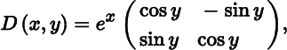
In either case, we refer to u and v as the real and imaginary parts of f, respectively. For example, the real and imaginary parts of the complex exponential function ez,
are given by
We say that f is complex differentiable at c if the limit
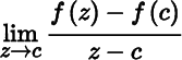
exists. (Recall that the ratio of two complex numbers is well‐defined.) Let us denote the derivative of the real‐valued vector function (u, v)′ with respect to its arguments x and y by
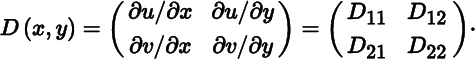
For example, for the complex exponential function defined in (40),
from which we see that D11 = D22 and D21 = −D12. These equalities are no coincidence as we shall see in a moment.
An immediate consequence of Theorem 5.14 are the Cauchy‐Riemann equations,
which we already saw to be true for the complex exponential function.
Theorem 5.14 tells us that a necessary condition for f to be complex differentiable at c is that the four partials Dij exist at c and satisfy the Cauchy‐Riemann equations. These conditions are not sufficient, because the existence of the four partials at c does not imply that the partials are continuous at c or that they exist in a neighborhood of c (see Section 5.9), so the functions u and v are not necessarily differentiable at c. If, however, u and v are differentiable at c and obey the Cauchy‐Riemann equations, then f is complex differentiable at c.
What happens if u and v are differentiable and the Cauchy‐Riemann equations are not satisfied? This can certainly happen as the example
shows. Letting c = a + ib, we have
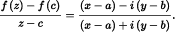
For y = b and x → a this ratio converges to 1, but for x = a and y → b it converges to −1. Hence, the limit does not exist and ![]() is not complex differentiable, despite the fact that u(x, y) = x and v(x, y) = −y are both differentiable. The problem is that the Cauchy‐Riemann equations are not satisfied, because D11(c) = 1 and D22(c) = −1 and these are not equal. This example shows that for a complex derivative to exist it is not enough that f is ‘smooth’ at c, in contrast to the real derivative.
is not complex differentiable, despite the fact that u(x, y) = x and v(x, y) = −y are both differentiable. The problem is that the Cauchy‐Riemann equations are not satisfied, because D11(c) = 1 and D22(c) = −1 and these are not equal. This example shows that for a complex derivative to exist it is not enough that f is ‘smooth’ at c, in contrast to the real derivative.
Now consider again the complex exponential function ez. The four partial derivatives Dij exist and are continuous everywhere in ℝ2, and hence u and v are differentiable (Theorem 5.7). In addition, they satisfy the Cauchy‐Riemann equations. Hence, the derivative Df(z) exists for all z and we have, by Theorem 5.14,
showing that, as in the real case, the exponential function equals its own derivative.
A function (real or complex) is analytic if it can be expressed as a convergent power series in a neighborhood of each point in its domain. For a complex‐valued function, differentiability in a neighborhood of every point in its domain implies that it is analytic, so that all higher‐order derivatives exist in a neighborhood of c. This is in marked contrast to the behavior of real‐valued functions, where the existence and continuity of the first derivative does not necessarily imply the existence of the second derivative.
Exercises
- 1. Show that f(z) = z2 is analytic on ℂ.
- 2. Consider the function f(z) = x2 + y + i(y2 − x). Show that the Cauchy‐Riemann equations are only satisfied on the line y = x. Conclude that f is complex differentiable only on the line y = x, and hence nowhere analytic.
- 3. Consider the function f(z) = x2 + y2. Show that the Cauchy‐Riemann equations are only satisfied at x = y = 0. Conclude that f is only complex differentiable at the origin, and hence nowhere analytic.
MISCELLANEOUS EXERCISES
- Consider a vector‐valued function f(t) = (cos t, sin t)′, t ∈ ℝ. Show that f(2π) − f(0) = 0 and that ||
Df(t) || = 1 for all t. Conclude that the mean‐value theorem does not hold for vector‐valued functions. - Let S be an open subset of ℝn and assume that f : S → ℝm is differentiable at each point of S. Let c be a point of S, and u a point in ℝn such that c + tu ∈ S for all t ∈ [0, 1]. Then for every vector a in ℝm, there exists a θ ∈ (0, 1) such that
where Df denotes the m × n matrix of partial derivatives Djfi(I = 1, …, m; j = 1, …, n). This is the mean‐value theorem for vector functions.
3. Now formulate the correct mean‐value theorem for the example in Exercise 1 and determine θ as a function of a.
BIBLIOGRAPHICAL NOTES
1. See also Dieudonné (1969), Apostol (1974), and Binmore (1982). For a discussion of the origins of the differential calculus, see Baron (1969).
6. There even exist functions which are continuous everywhere without being differentiable at any point. See Rudin (1964, p. 141) for an example of such a function.
14. For modified versions of the mean‐value theorem, see Dieudonné (1969, Section 8.5). Dieudonné regards the mean‐value theorem as the most useful theorem in analysis and he argues (p. 148) that its real nature is exhibited by writing it as an inequality, and not as an equality.
17. See Needham (1997) for a lucid introduction to complex differentiation, and Hjørungnes and Gesbert (2007) for a generalization of real‐valued differentials to the complex‐valued case using complex differentials.